Multi-Output Based Hybrid Integrated Models for Student Performance Prediction

Abstract

In higher education, student learning relies increasingly on autonomy. With the rise in blended learning, both online and offline, students need to further improve their online learning effectiveness. Therefore, predicting students’ performance and identifying students who are struggling in real time to intervene is an important way to improve learning outcomes. However, currently, machine learning in grade prediction applications typically only employs a single-output prediction method and has lagging issues. To advance the prediction of time and enhance the predictive attributes, as well as address the aforementioned issues, this study proposes a multi-output hybrid ensemble model that utilizes data from the Superstar Learning Communication Platform (SLCP) to predict grades. Experimental results show that using the first six weeks of SLCP data and the Xgboost model to predict mid-term and final grades meant that accuracy reached 78.37%, which was 3–8% higher than the comparison models. Using the Gdbt model to predict homework and experiment grades, the average mean squared error was 16.76, which is better than the comparison models. This study uses a multi-output hybrid ensemble model to predict how grades can help improve student learning quality and teacher teaching effectiveness.

1. Introduction

With the rapid development of the Internet, online education has grown quickly, meeting the urgent needs of the public for home-based learning and educational development through media such as the Internet. The core features of online education are mobility, interactivity, intelligence, personalization, and globalization. Online education has significant advantages in promoting the co-construction and sharing of educational resources and promoting educational equity and is a trend that has been widely applied [1]. Currently, online education mostly relies on online learning platforms, such as China’s MOOC and SLCP, which provide students with rich learning resources. However, if students do not pay attention to the accumulation of knowledge during their regular study, the failure rate in their final exams will increase, and their learning quality is worrying. In the teacher’s evaluation process, both process evaluation and result evaluation are particularly important, especially in online learning where teachers cannot better pay attention to students’ learning progress, resulting in poor process evaluation results. Courses that include teaching practice, experiments and homework reflect to some extent whether students have a good learning attitude and ability in the learning process. In this case, it is particularly important to provide a reliable combined process and result-oriented grade prediction method.

Currently, research on predicting student grades has achieved certain results, but still faces the following issues:

Grade prediction is usually conducted late, leaving students and teachers with limited time to change study methods or intervene, resulting in teachers only being able to provide guidance to students who are struggling, but are unable to give more attention to high-performing students.

Student grade prediction is usually a single-output and results-oriented prediction, such as only predicting final grades, which cannot predict students’ learning progress at different stages throughout the semester. This lack of information makes it difficult for teachers to accurate and effectively intervene and provide guidance to students.

To address these issues, this study proposes a multi-output prediction method to predict students’ stage performances from the 7th week to the end of the semester, including midterm grades, homework grades, experiment grades, and final grades. These grades can more fully reflect students’ learning progress.

The main contributions of this study are reflected in the following two aspects:

The time for grade prediction was moved up to the 7th week, providing teachers with more time for teaching intervention and enabling personalized learning for students.

Additionally, more attributes could now be predicted, including homework, mid-term, experiment, and final exam scores, facilitating the teachers’ understanding of students’ learning status and integrating process and outcome evaluations.

The organization of this study is as follows. First, related research is introduced. Second, the framework and experimental process for predicting student grades are detailed. Next, the experimental results are presented, followed by a summary of the study.

2. Related Work

Student grade prediction has always been a hot topic in educational data mining. Currently, there have been some achievements in predicting learning outcomes. Machine learning-based grade prediction is usually divided into classification prediction and regression prediction. Classification prediction predicts the grade level, while regression prediction predicts the specific grade value. Mustafa Yalcin et al. [2] proposed a new model based on machine learning algorithms to predict the final exam scores of college students. By collecting mid-term scores and student data from departments and colleges at a state university, they classified final exam scores into four categories. After comparing the performance of various algorithms such as random forest, k-nearest neighbors, classification neural network model, and support vector machine, they selected the optimal model to predict students’ final exam scores. A random forest and classification neural network model had an accuracy rate of 70–75% and only used three dimensions and three attributes, reducing the difficulty of data collection. Xu Huan et al. [3] proposed an improved IDA-SVR (Support Vector Regression Optimized by Dual Algorithms) algorithm to predict student performance scores, with a mean squared error of 0.0089, which was better than other algorithms such as decision trees and SVR. Their data included 18 attributes in four dimensions: basic information, interests, classroom behavior, and extracurricular behavior, and had diverse data types. Muhammad Hazique Bin Roslan et al. [4] predicted English and mathematics scores of 16-year-old Malaysian students using their past academic performance, demographics, and psychological information. They also explored the main factors that affect students’ English and mathematics scores and the relationship between them. The experiment showed that decision trees had the best performance in predicting English scores, and Bayesian algorithms had the best performance in predicting mathematics scores, with an accuracy rate of 87.1% and 83.9%, respectively, and found that there was a certain relationship between mathematics and English scores. Xiaoyong Li et al. [5] proposed an end-to-end deep learning model that could automatically extract features from heterogeneous student behavior data to predict learning outcomes. They collected and experimented with daily behavior data from 8228 students, and the experiment showed that the accuracy of this deep learning model in grade prediction was better than traditional machine learning algorithms. In their study, Yangyang Luo et al. [6] attempted to construct a predictive model of the one-to-one relationship between student online behavior and academic performance using five machine learning algorithms. However, they found it difficult to obtain good predictive results, with the highest accuracy of the predictive model being able to predict 74.7% of students correctly in all mixed courses. There were significant differences in the predictive accuracy of students with different learning outcomes. Students with grades A (90–100) and B (80–89) had a higher predictive accuracy, reaching 80.6% and 85.3%, respectively. However, the highest predictive accuracy for students with grades of C (70–79) or below was only 63%. Ashima Kukkar et al. [7] used a combination of a four-layer stacked long short-term memory (LSTM) network, random forest (RF), and gradient boosting (GB) techniques to predict whether students passed or failed, achieving an accuracy rate of 96% by verifying with the OULAD dataset. Wenjing Ban et al. [8] designed a multi-algorithm online learning performance prediction framework that integrated neural networks, decision trees, K-nearest neighbors, random forests, and logistic regression algorithms to predict online learning performance. They utilized Weka software to automatically implement the multi-algorithm fusion prediction function and conducted a predictive performance analysis. This multi-algorithm fusion prediction was more accurate than a single algorithm, and the precision reached 78.9%. Compared with the predictive accuracy of every single algorithm trained by a single classifier, the multi-algorithm fusion prediction improved by 2.9%, 5.5%, 2.7%, 2.7%, and 5.5% in various evaluation indicators. Ortiz et al. [9] constructed a network through interactive data from the student management system and found that the network characteristics of successful students were fractal, while failed students were exponential models. They used a deep learning network to predict student performance, with an accuracy rate of 94%. Yu Jun et al. [10] made full use of students’ course history information and the correlation between multiple target courses to predict students’ different course grades, identifying student risk situations before the course. Yu Jun et al.’s research could predict students’ performance before the course, but it only focused on result-oriented prediction and did not achieve process-oriented performance prediction.

The existing research on predicting student performance typically focuses on single-output predictions, such as predicting the final exam score or overall grade. Such predictions can only provide a limited understanding of a student’s learning progress, and interventions based on these predictions are often short-term and not very effective. Furthermore, models that can make early predictions tend to be result-oriented rather than process-oriented. Building upon the research by Yu Jun et al., this study aimed to transform historical data from multiple courses into a single course, thereby converting the predictions of grades in multiple courses into process-oriented predictions of grades in a single course. This approach enables teachers to better understand a student’s learning progress and facilitates effective and targeted teaching interventions.

3. Materials and Methods

3.1. Multi-Output Prediction Model Framework

The objective of this study was to identify a model that could effectively combine multi-label classification prediction and multi-label discrete value prediction of tasks based on multiple outputs. This model was then used for process-oriented and result-oriented grade prediction. The model framework consists of four main stages, as shown in Figure 1: In the first stage, data on the course “C++ programming” was obtained from the SLCP, and the corresponding data were merged and preliminarily cleaned. The input data for this model framework included student names, task click-through rates, video viewing times, and other data. In the second stage, the data were pre-processed and model designed, including handling missing data, data normalization, and text discretization. Different models are selected for classification, and discrete models to perform predictions. In the third stage, different models were compared using the same evaluation metrics, and the model with the best evaluation metric was selected for the final prediction. In the fourth stage, the prediction results were visualized. Each stage is described in detail in the following sections.

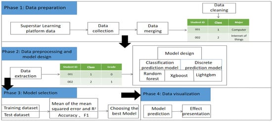
Figure 1. Model framework.

3.2. Data Set

This study presents experimental data collected from 122 students enrolled in a “C++ Programming” course at a university in Chongqing, China, from March to July 2022. The students were required to complete regular assignments and experiments and were assessed based on their midterm and final exam scores using the SLCP. The dataset includes 32 attributes, such as name, student ID, major, class, number of completed tasks, homework scores, experiment scores, and time, as detailed in Table 1 and Table 2. In these attributes, all scores are arranged in chronological order to distinguish the learning status. In this study, 70% of the data were used for training and 30% for testing.

Table 1. Basic situation of students.

Serial Number	Characteristic Name	Data Type	Characteristic Meaning
1	name	varchar	name
2	student ID	varchar	student number
3	class	varchar	class
4	major	varchar	major
5	faculty	varchar	department

Table 2. Student interaction.

Serial Number	Characteristic Name	Data Type	Characteristic Meaning	Time
1	task_click	int	number of tasks completed
2	view_time	double	video viewing duration
3	discuss_count	int	number of discussions
4	study_count	int	learning times
5	sign	int	sign-in times
6	experiment1	double	experiment result 1	1 March 2022
7	theory1	double	theoretical score 1	6 March 2022
8	experiment2	double	experiment result 2	11 March 2022
9	experiment3	double	experiment result 3	16 March 2022
10	experiment4	double	experiment result 4	21 March 2022
11	theory2	double	theoretical score 2	26 March 2022
……	……	……	……	……
32	end_score	double	final exam	1 July 2022

3.3. Data Preprocessing

Due to the fact that raw data are “dirty” data, in order to reduce the impact of low-quality data on model predictions during the process of model construction, scientific data processing methods such as scaling and one-hot encoding were selected [11]. In this study, the primary issue observed with the data was the presence of missing values. Three methods of filling in missing values—0 fillings, mean filling, and random forest filling—were compared to select the most appropriate method for model construction. Furthermore, the midterm and final exam scores were classified into two categories: scores ranging from 60 to 100 were represented as 1, indicating a passing grade, while scores below 60 were represented as 0, indicating a failing grade. The ratio of samples with scores of 0 and 1 in the midterm exam was 0.54:1, while the ratio in the final exam was 1.26:1, indicating a basic balance between the data. Since machine learning algorithms cannot handle character data, the character types in the data need to be converted accordingly. In addition, since the values in each column attribute are on different scales, the data need to be normalized to the range of [0, 1]. The formula for normalization is as follows: where max represents the maximum value and min represents the minimum value [12].

$${\mathrm{X}}^{\prime }=\frac{\mathrm{x}-\min }{\max -\min }$$

(1)

Table 3 presents the detailed performance of students in the C++ Programming course. The passing rates for the midterm and final exams were 64.75% and 44.26%, respectively. In the hybrid online and offline learning of this course, the low pass rate in the final exam could significantly reduce students’ enthusiasm for learning, indicating the need for corresponding teaching interventions. The overall mean and standard deviation (std) of the original data and missing values, filled by 0 fillings, mean filling, and a random forest algorithm filling, are shown in Figure 2 and Figure 3, respectively. The mean value was lowest when using the 0-filling method, and the standard deviation value was lowest when using the mean-filling method.

Table 3. Student performance.

Major	Qualified in the Interim	Intermediate Unqualified	Qualified at the End of the Period	Unqualified at the End of the Period	Total
Computer Science and Technology	29	15	16	28	44
Software engineering	30	9	29	10	39
Intelligent science and technology	20	17	9	28	37
Other	0	2	0	2	2
Total	79	43	54	68	122
Percentage	64.75%	35.25%	44.26%	55.74%

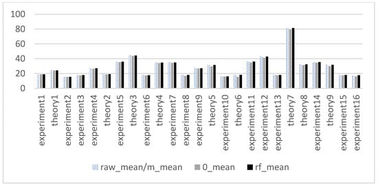
Figure 2. Average value of data.

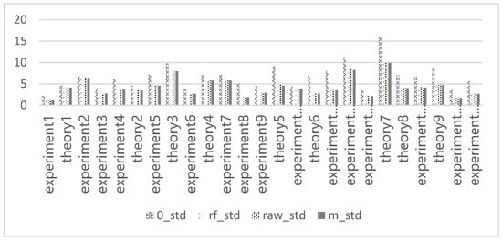
Figure 3. Standard deviation of data.

3.4. Model Design

This study collected students’ learning data from the first six weeks and aimed to predict their process and outcome scores from the seventh week to the final exam. Currently, ensemble models are widely used in machine learning and have shown good performance. Ensemble models combine individual machine learning models in different ways to construct a model that has better performance and generalization ability than a single machine learning model [13]. Representative models in this category include Adboost, Gdbt, Randomforest, Xgboost, and Lightgbm. Different ensemble learning algorithms may perform differently on the same dataset. Therefore, this study compared the performance of different ensemble models to select the best-performing one for predicting student scores. The model prediction process is shown in Figure 4.

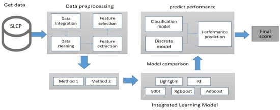
Figure 4. Multi-output prediction model.

Random forest model: It is a type of ensemble classifier based on machine learning, which combines multiple decision trees. It uses the number of decision trees on different subsets to find the best features and achieve higher accuracy. When dealing with regression problems, the output value is the mean of all the trees, and for classification problems, it uses majority voting to output the result. Random forest not only has the efficiency of decision trees but also prevents overfitting [14].

Xgboost model: It is an advanced algorithm specifically designed for extreme gradient boosting. It uses CART as the basic classifier, and multiple related decision trees make joint decisions. The input sample of the next decision tree is related to the training and prediction results of the previous decision tree. It improves ordinary gradient boosting by determining the depth of decision trees as weak learners to prevent overfitting, adding a penalty parameter to prevent the depth of decision trees from being too large, reducing the proportion of nodes on the decision tree, and adding randomization parameters to achieve optimal learning [15].

Lightgbm model: It is an improved framework based on decision tree algorithms released by Microsoft in 2017. Lightgbm’s main feature is its gradient-based one-sided sampling (GOSS) decision tree algorithm, exclusive feature bundling (EFB), and histogram and leaf-oriented growth strategies with depth limits [16].

Adboost model: It is a machine learning algorithm proposed by Freund and Schapire. It can be combined with other algorithms to form more complete algorithms. To improve the model’s performance, it does not assign the same weight to the data in the model but increases the weight of erroneous data. In the next iteration, these data will be given more attention, resulting in higher performance [17].

Gdbt model: It constructs a series of weak learners and continuously increases or enhances relatively weak learners. The model is trained based on the residual generated by the previous predicted value, and each decision tree model is sequentially constructed according to the gradient descent direction of the loss function. The loss function describes the accuracy of the model, and the larger the loss function’s value, the worse the trained model’s predictive ability is [18].

There are two methods for predicting multiple output attributes. Method 1 (Figure 5) divides multiple outputs into multiple single outputs for prediction, and the output between each output is independent. Method 2 (Figure 6) includes the predicted single attributes into the known data to predict the next attribute, and there is a certain relationship between the outputs. This study compares the two methods to select the optimal method for prediction and, according to different methods, select the appropriate model. The model selection process is shown in Algorithm 1.

Algorithm 1: Multi-output model under different methods

Input: training data

Output: mid-term grade, homework grade, experiment grade, final grade

1 Start

2 Import necessary packages and read data

3 Perform data preprocessing

3.1 Feature attribute extraction

3.2 Missing value padding

3.3 Text data conversion

4 Use classifier/regression to predict

4.1 Use method 1 to predict different models

4.2 Use method 2 to predict different models

4.2 Select model parameters according to the evaluation index using tenfold cross validation

5 Compare the effects of different models according to evaluation indicators

6 Combine the most appropriate model for prediction

7 End

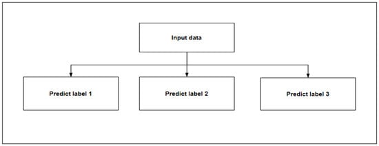
Figure 5. Method 1.

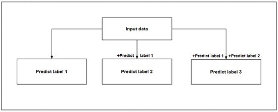
Figure 6. Method 2.

3.5. Model Evaluation

This study is based on multi-output prediction, with evaluation metrics including classification evaluation and discrete value evaluation. The classification metrics selected are accuracy, precision, recall, and F1 score. In machine learning, the confusion matrix (Table 4) is the most basic, intuitive, and computationally simple method for measuring the accuracy of classification models. For discrete value prediction metrics, this study selects the mean squared error average, mean absolute error average, and R² score average. By comparing the evaluation metrics with each other, this paper selects the best model for prediction.

Table 4. Confusion matrix.

	True Value
Estimate		p	n	Total
	P’	True positive (TP)	False positive (FP)	P’
	n’	False negative (FN)	True negative (TN)	N’
	Total	P	N

The performance index of the confusion matrix is determined by the accuracy rate, precision rate, recall rate, and F1 value [19].

Accuracy: the ratio of the correct number of samples to the total number of samples, formula: (A) = (TP + TN)/(P + N)

Precision: the ratio of the number of positive samples was correctly predicted to the total number of positive samples predicted, formula: (P) = TP/(TP + FP)

Recall: reflect how many positive cases are divided into positive cases, formula: (R) = TP/(TP + FN)

F1 value: it is used to measure the accuracy of the two-category model, the harmonic value of the precision rate, and the recall rate. Formula: F1 = 2 × TP/(2 × TP + FN + FP)

The mean of the mean square error: the average value of the sum of squares on the difference between the predicted value and the true value of each column of attributes. The formula is as follows:

$$MSE\_a=\frac{1}{n}{\displaystyle \sum _{i=1,j=1}^n{(\stackrel{}{{\hat{y}}_{ij}-}{y}_{ij})}^2}$$

(2)

The mean of mean absolute error: the average value of the average error between the predicted value and the true value of each column can be expressed through the formula as follows:

$$MAE\_a=\frac{1}{n}{\displaystyle \sum _{i=1,j=1}^n|}{\hat{y}}_{ij}-y_{ij}{|}^2$$

(3)

The average value of R² score: the average value of the square of the R coefficient of each column of attributes is expressed through the formula as follows:

$$R^2\_a=\frac{{\displaystyle \sum _{i=1,j=1}^n{({\hat{y}}_{ij}-\stackrel{\_}{y_{ij}})}^2}}{{\displaystyle \sum _{i=1,j=1}^n{({\hat{y}}_{\mathrm{ij}}-\stackrel{\_}{y_{ij}})}^2}}$$

(4)

3.6. Model Parameter Configuration

For ensemble models, selecting appropriate parameters can enhance the model’s ability. In this study, we used GridSearchCV (grid search method) in the machine learning library scikit-learn during model training and combined it with ten-fold cross-validation to select the best parameters by comparing the accuracy and mean squared error. Due to a large number of predictions, the top three models with better performance were selected for each prediction, and their respective optimal parameters are presented in Table 5.

Table 5. Model parameter.

Model	Parameter Settings	Accuracy/MSE_a
m_xgboost(midterm exam)	learning_rate=0.1,max_depth=2, n_estimators=100,max_delta_step=0.2	0.7837
0_xgboost(midterm exam)	learning_rate=0.9,n_estimators=50, min_child_weight=2,max_depth=2	0.7567
0_gdbt(midterm exam)	random_state=40,learning_rate=0.55,n_estimators=100	0.7567
m_xgboost(final exam)	max_depth=3,learning_rate=0.19,n_estimators=100, min_child_weight=1,max_delta_step=0.4	0.7837
r_xgboost(final exam)	learning_rate=0.70,n_estimators=100, min_child_weight=1,max_delta_step=0.2	0.7567
0_xgboost(final exam)	learning_rate=0.90,max_depth=8, min_child_weight=1,max_delta_step=0.5	0.7297
m_gdbt(process grade)	random_state=40,learning_rate=0.01,subsample=0.2	16.7699
m_randomforests(process grade)	random_state=40,max_depth=2,min_samples_leaf=10	17.1784
r_gdbt(process grade)	random_state=40,learning_rate=0.01,subsample=0.2	17.7929

3.7. Model Comparison

The missing values in the dataset of this study were handled using zero imputation, mean imputation, and random forest imputation methods, and two techniques were employed for prediction. For the classification model, the selection of the model was primarily based on accuracy, with other evaluation metrics considered supplementary. For the discrete model, the selection of the model was primarily based on the mean squared error of the mean, with other evaluation metrics considered supplementary.

3.7.1. Comparison of Classification Models

Table 6 and Figure 7 depict the performance evaluation of three different imputation methods when predicting scores during the forecast period, wherein the Xgboost model achieved an accuracy of 78.37% under the mean imputation method, which was 2–5% higher than other models. Furthermore, the recall and F1 score of the Xgboost model was superior to all other models, while its precision was lower than the best model by 2%. Combining the information presented in the tables and figures, the Xgboost model under the mean imputation method demonstrated the most favorable performance in predicting scores during the forecast period.

Table 6. Evaluation indicators of mid-term performance prediction model.

Model	Accuracy	Precision	Recall	F1
m_xgboost	0.7837	0.8148	0.88	0.8461
0_xgboost	0.7567	0.8333	0.8	0.8163
0_gdbt	0.7567	0.8076	0.84	0.8235
m_lgb	0.7567	0.8333	0.8	0.8163
m_gdbt	0.7567	0.8076	0.84	0.8235
r_lgb	0.7567	0.8333	0.8	0.8163
r_gdbt	0.7567	0.8333	0.8	0.8163
0_lgb	0.7297	0.8	0.8	0.8
m_randomforests	0.7297	0.7586	0.88	0.8148
r_randomforests	0.7297	0.7586	0.88	0.8148
0_randomforests	0.7027	0.7333	0.88	0.8
0_adboost	0.7027	0.7692	0.8	0.7843
m_adboost	0.7027	0.7692	0.8	0.7843
r_xgboost	0.7027	0.7916	0.76	0.7755
r_adboost	0.7027	0.75	0.84	0.7924

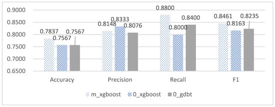
Figure 7. The first three types of model evaluation indicators of mid-term performance accuracy.

As demonstrated in Table 7 and Figure 8, under the random forest imputation method, the Gdbt, Adboost, and Lightgbm models attained the same accuracy evaluation indicator of 75.67%, which was 2–10% higher than other models in terms of accuracy. However, the Lightgbm model outperformed other models in terms of their recall and F1 score, while its precision was approximately 2% lower than the optimal model. Based on the comprehensive information presented in the tables and figures, the Lightgbm model under the random forest imputation method exhibited the most favorable performance in predicting end-of-period scores.

Table 7. Evaluation indicators of final performance prediction based on method 1.

Model	Accuracy	Precision	Recall	F1
r_lgb	0.7567	0.6875	0.7333	0.7096
r_gdbt	0.7567	0.7142	0.6666	0.6896
r_adboost	0.7567	0.7142	0.6666	0.6896
m_xgboost	0.7297	0.6470	0.7333	0.6875
m_gdbt	0.7297	0.6666	0.6666	0.6666
r_xgboost	0.7297	0.6923	0.6	0.6428
0_xgboost	0.7027	0.6428	0.6	0.6206
0_gdbt	0.7027	0.6666	0.5333	0.5925
m_randomforests	0.7027	0.6428	0.6	0.6206
m_lgb	0.7027	0.6111	0.7333	0.6666
m_adboost	0.7027	0.6428	0.6	0.6206
0_randomforests	0.6756	0.6	0.6	0.6
0_lgb	0.6756	0.6	0.6	0.6
r_randomforests	0.6756	0.6	0.6	0.6
0_adboost	0.6486	0.5625	0.6	0.5806

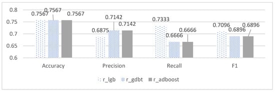
Figure 8. Evaluation indicators of the first three types of models based on method 1.

As shown in Table 8 and Figure 9, the Xgboost model under the mean imputation method in Method 2 outperformed other models by 2–10% in terms of accuracy and was approximately 3% higher in accuracy than the best-performing Lightgbm model in Method 1. Moreover, it demonstrated superior performance in other evaluation indicators compared to the Lightgbm model in Method 1. Based on the information presented in the tables and figures, selecting the predictive model in Method 2 generally yields better results than the predictive model in Method 1.

Table 8. Evaluation of final grade prediction model based on method 2.

Model	Accuracy	Precision	Recall	F1
m_xgboost	0.7837	0.7058	0.8	0.75
r_xgboost	0.7567	0.7142	0.6666	0.6896
0_xgboost	0.7297	0.6666	0.6666	0.6666
0_gdbt	0.7297	0.6666	0.6666	0.6666
m_gdbt	0.7297	0.6666	0.6666	0.6666
m_adboost	0.7297	0.6666	0.6666	0.6666
0_lgb	0.7027	0.6111	0.7333	0.6666
0_adboost	0.7027	0.6	0.8	0.6857
m_lgb	0.7027	0.6111	0.7333	0.6666
r_lgb	0.7027	0.625	0.6666	0.6451
r_gdbt	0.7027	0.625	0.6666	0.6451
r_adboost	0.7027	0.625	0.6666	0.6451
0_randomforests	0.6756	0.6	0.6	0.6
m_randomforests	0.6756	0.5882	0.6666	0.625
r_randomforests	0.6756	0.6	0.6	0.6

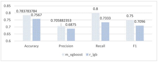
Figure 9. Comparison of Xgboost model under method 2 and Lightgbm model under method 1.

Taking into account the comparison of the aforementioned evaluation indicators, this paper selected the Xgboost model under the mean imputation method to predict mid-term scores and used Method 2 to predict end-of-period scores in the selection of classification models.

3.7.2. Comparison of Discrete Models

As shown in Table 9, the performance evaluation of score prediction under mean imputation and random forest imputation methods was superior to the evaluation indicators of 0 imputations. Moreover, the score prediction indicators under Method 2 were generally better than the evaluation indicators of Method 1. Based on the comprehensive evaluation of the three indicators, this paper selected the Gdbt model under mean imputation for discrete model prediction.

Table 9. Evaluation indicators of method I and method 2.

Model	Process Performance Prediction (Method 1)			Process Performance Prediction (method 2)
	MSE_a	MAE_a	R2_a	MSE_a	MAE_a	R2_a
m_gdbt	17.737	2.8383	0.0167	16.769	2.7417	0.0375
m_randomforests	17.674	2.8063	−0.001	17.178	2.8562	0.0052
r_gdbt	18.086	2.9610	−0.005	17.792	2.8889	0.0050
m_lgb	18.132	2.8617	0.0058	18.037	2.8769	0.0057
m_adboost	18.944	2.9401	−0.106	18.259	2.8527	−0.073
r_randomforests	18.478	2.9623	−0.011	18.489	2.9722	−0.006
r_lgb	18.903	2.9905	−0.004	18.794	2.9871	−0.000
r_adboost	20.139	3.1394	−0.124	19.707	2.9475	−0.161
m_xgboost	24.787	3.3564	−0.472	22.362	3.1556	−0.348
r_xgboost	24.290	3.3235	−0.393	23.006	3.3048	−0.407
0_xgboost	48.162	4.3520	0.4434	37.588	4.0346	0.4600
0_adboost	47.694	3.6535	0.4937	43.786	3.5881	0.4735
0_gdbt	48.850	4.3454	0.3914	47.318	4.1756	0.4171
0_randomforests	56.879	4.3626	0.3538	49.833	4.0620	0.4664
0_lgb	79.682	5.2129	0.1041	76.234	4.8797	0.1409

3.8. Model Determination

Based on the comparison of the models presented above, the final selection for this study is as follows: under the mean imputation scenario, Method One using the Xgboost model was chosen to predict the midterm scores, Method Two using the Xgboost model was selected to predict the final scores, and the Gdbt model was chosen to predict the grades for assignments and experiments.

4. Experimental Setup

All data processing, modeling, and analysis in this study were conducted using PyCharm Community Edition 2021.3.2, which was developed by the JetBrain company in the Czech Republic, and Python 3.8. The environment in which these processes were carried out was an Intel(R) Core(TM) i5-8300H processor, which was developed by Intel Corporation in Santa Clara, CA, USA, and had 8 GB of RAM, running on the Windows 10 (64-bit) operating system, which was developed by Microsoft Corporation in Redmond, WA, USA. The data used in this study were obtained from the SLCP. During the data processing phase, the pandas’ module was utilized for missing value handling, text discretization, and other processing tasks. Multiple ensemble learning models were called using the scikit-learn module for data modeling, and parameter selection was performed using GridSearchCV. The detailed parameters are shown in Table 1 in Section 3.6. For data analysis and visualization, the matplotlib module was utilized.

5. Experimental Results and Discussion

The experiments of this study were conducted from November 2022 to January 2023, with the aim of predicting the process grades and learning status of students from their 7th week to the final exam. After model prediction, good results were obtained, as shown in Figure 10: the blue line represents the true grades, and the orange line represents the predicted grades. For 109 students, both the midterm and final exam grades were correctly predicted, and other experimental grades and homework grades were well-fitted with small errors. However, there was some deviation between the predicted and actual values when predicting the score for Experiment 12. Overall, the continuous prediction effect was satisfactory. Considering the prediction of all discrete values, as shown in Figure 11, the fit between the true and predicted grades for Theoretical 7 was relatively poor compared to other grades, possibly due to the large range of values for Theoretical 7. However, good simulations of the student’s true grades were obtained for other discrete value predictions. For the prediction of midterm and final exam grades, the accuracy rates of both models in Section 3.7.1 were 78.37%, as shown in Figure 12 and Figure 13, where the patterns represent the true values, and the solid colors represent the predicted values.

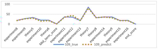
Figure 10. Overall prediction effect of No. 109 students.

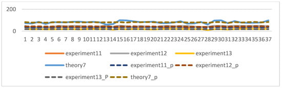
Figure 11. Prediction effect of discrete value.

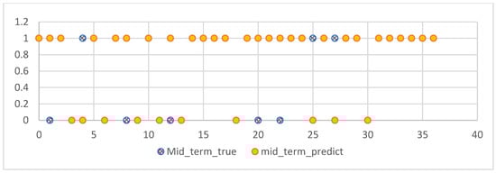
Figure 12. Prediction of mid-term results.

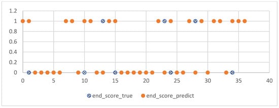
Figure 13. Final score forecast.

6. Conclusions

This study utilizes learning data from the first six weeks of a course platform to predict students’ homework, experiment, midterm, and final scores six weeks later, achieving good results. This provides timely warnings for students who have difficulty learning and personalized guidance for those who perform well. Additionally, teachers can intervene and provide effective teaching guidance based on students’ performance in various stages of the course, thereby improving teaching efficiency and quality. Previous grade predictions have focused more on whether students can pass exams rather than on paying attention to their learning processes. For practical courses, experiments are particularly important, and this model can better predict students’ process performance. With the help of the prediction system, teachers can better understand students’ learning processes and make precise teaching interventions, providing different recommendations for students who have difficulty learning and those who excel. However, there are also many shortcomings in this article, such as the small and unrepresentative dataset used. Currently, the model can only predict scores on this single course platform, and the generalization ability of the model needs to be improved. In addition, teachers need to remind students enough to accumulate good data in the first six weeks of the course platform to effectively and accurately predict students’ scores. In this study, the second method’s predictive evaluation indicators were generally better than those of the first method. However, due to the small amount of data processed, whether the second method is more effective than the first method requires further exploration in future real-world applications.

In future grade predictions, it is hoped that this model will be able to predict students’ grades and learning status in each stage of their course when students start school. The generalization ability and applicability of the model need to be significantly improved so that it can be more widely used in various fields to provide teaching warnings and interventions and improve teaching efficiency and quality.

References

- Xiao, R.; Qu, J.; Wang, H.; Wang, M. Research on Clustering, Causes and Countermeasures of College Students’ Online Learning Behavior. Softw. Guide. 2022, 6, 230–235. [Google Scholar]
- Yağcı, M. Educational data mining: Prediction of students’ academic performance using machine learning algorithms. Smart Learn. Environ. 2022, 9, 1–19. [Google Scholar] [CrossRef]
- Xu, H. Prediction of Students’ Performance Based on the Hybrid IDA-SVR Model. Complexity 2022, 2022, 1845571. [Google Scholar] [CrossRef]
- Roslan, M.H.B.; Chen, C.J. Predicting students’ performance in English and Mathematics using data mining techniques. Educ. Inf. Technol. 2022, 28, 1427–1453. [Google Scholar] [CrossRef] [PubMed]
- Li, X.; Zhang, Y.; Cheng, H. Student achievement prediction using deep neural network from multi-source campus data. Complex Intell. Syst. 2022, 8, 5143–5156. [Google Scholar] [CrossRef]
- Luo, Y.; Han, X. Exploring the interpretability of the mixed curriculum student achievement prediction model. China Distance Education. 2022, 6, 46–55. [Google Scholar]
- Kukkar, A.; Mohana, R.; Sharma, A.; Nayyar, A. Prediction of student academic performance based on their emotional wellbeing and interaction on various e-learning platforms. Educ. Inf. Technol. 2023, 1–30. [Google Scholar] [CrossRef]
- Ban, W.; Jiang, Q.; Zhao, W. Research on accurate prediction of online learning performance based on multi algorithm fusion. Modern Distance Education. 2022, 3, 37–45. [Google Scholar]
- Ortiz-Vilchis, P.; Ramirez-Arellano, A. Learning Pathways and Students Performance: A Dynamic Complex System. Entropy 2023, 25, 291. [Google Scholar] [CrossRef] [PubMed]
- Ma, Y.; Cui, C.; Yu, J. Multi-task MIML learning for pre-course student performance prediction. Front. Comput. Sci. 2020, 14, 1–10. [Google Scholar] [CrossRef]
- Shen, G.; Yang, S.; Huang, Z.; Yu, Y.; Li, X. The prediction of programming performance using student profiles. Educ. Inf. Technol. 2022, 28, 725–740. [Google Scholar] [CrossRef]
- Yekun, E.A.; Haile, A.T. Student performance prediction with optimum multilabel ensemble model. J. Intell. Syst. 2021, 30, 511–523. [Google Scholar] [CrossRef]
- Kumar, A. Introduction and Practice of Integrated Learning: Principles, Algorithms and Applications. Beijing:Chem. Ind. Press. 2022, 2, 9–11. [Google Scholar]
- Wang, H.; Wang, G. Improving random forest algorithm by Lasso method. J. Stat. Comput. Simul. 2021, 91, 353–367. [Google Scholar] [CrossRef]
- Ma, M.; Zhao, G.; He, B. XGBoost-based method for flash flood risk assessment. J. Hydrol. 2021, 598, 126382. [Google Scholar] [CrossRef]
- Wang, Y.; Wang, T. Application of improved LightGBM model in blood glucose prediction. Appl. Sci. 2020, 10, 3227. [Google Scholar] [CrossRef]
- Heo, J.; Yang, J.Y. AdaBoost based bankruptcy forecasting of Korean construction companies. Appl. Soft Comput. 2014, 24, 494–499. [Google Scholar] [CrossRef]
- Zhang, C.; Zhang, Y.; Shi, X. On incremental learning for gradient boosting decision trees. Neural Process. Lett. 2019, 50, 957–987. [Google Scholar] [CrossRef]
- Zhou, Z. Machine Learning; Tsinghua University Press: Beijing, China, 2016; pp. 28–32. [Google Scholar]
Disclaimer/Publisher’s Note: The statements, opinions and data contained in all publications are solely those of the individual author(s) and contributor(s) and not of MDPI and/or the editor(s). MDPI and/or the editor(s) disclaim responsibility for any injury to people or property resulting from any ideas, methods, instructions or products referred to in the content. |
© 2023 by the authors. Licensee MDPI, Basel, Switzerland. This article is an open access article distributed under the terms and conditions of the Creative Commons Attribution (CC BY) license (https://creativecommons.org/licenses/by/4.0/).