Research on an Improved Method for Galloping Stability Analysis Considering Large Angles of Attack

Abstract

In view of the deficiency of the quasi-steady galloping critical wind speed calculation method based on the classical Den Hartog criterion, this paper proposes a quasi-steady galloping stability analysis method that considers the wind attack angle criterion (dC_V/dα) through theoretical analysis. Firstly, the tri-component force coefficients of a square-section model were measured through wind tunnel tests, and the galloping force coefficients calculated with three different galloping criteria (the dC_V/dα criterion, Den Hartog criterion, and Xie criterion) were compared and analyzed. Secondly, to further verify the reliability and applicability of the criteria proposed in this study, wind tunnel tests and numerical simulations were conducted on an H-shaped section. The verification results of the H-shaped section showed that under the action of the incoming flow at a large angle of attack of 70°, the maximum error of the classic Den Hartog criterion could reach about 44%. This study used the dCV/dα criterion while considering the large angle of attack of the incoming flow, and its calculation error could be controlled within 10%. At the same time, the numerical simulation showed that there was serious aerodynamic instability in this section under the critical wind speed. A pair of periodic vortex structures were formed in the wake region of the H-shaped section, resulting in constant generation and separation phenomena, which induced structural instability.

1. Introduction

For a long time, the wind-resistant stability of bridges has attracted wide attention in the wind engineering community. In particular, the galloping of a bridge is a speed-dependent, damping-controlled, single-degree-of-freedom phenomenon of aeroelastic instability and it easily occurs when the aspect ratio of a bluff’s body section is small, such as in a main steel girder, a steel bridge tower, cables, box-type arch ribs of long-span steel arch bridges, etc. This is a kind of low-frequency (from 0.25 to 1.25 Hz), high-amplitude (from a few centimeters to 6 m), and self-excited scattered vibration [1]. Therefore, once galloping occurs, it causes serious damage to bridge structures [2].

To study galloping, researchers generally use wind tunnel tests, numerical simulations, and theoretical analysis methods. Robertson et al. used a numerical simulation method to simulate the transverse and torsional directions of rectangular sections at different aspect ratios with low Reynolds numbers. The results of the numerical simulation were consistent with the quasi-steady-state analysis theory of galloping [3]. Alonso et al. conducted static and dynamic wind tunnel tests to evaluate the galloping stability of a section, and the results showed that the static and dynamic test results were in good agreement [4,5]. Then, they conducted relevant research on the galloping instability of two-dimensional objects with elliptical cross sections and attempted to establish relationships between different parameters based on a stability map of the cross sections [6]. Barrero-Gil studied the phenomenon of galloping with a single degree of freedom in the lateral direction through the quasi-steady-state assumption, analyzed the phenomenon of hysteresis in galloping, and obtained an approximate solution to the model by assuming that the aerodynamic force and damping force were much smaller than the inertial force and stiffness force [7]. Abdelkefi et al. proposed the concept of energy harvesting by using the galloping behavior and conducted related research on the galloping behavior of differently shaped sections [8]. It was pointed out that it is necessary to carry out a coupling analysis on a galloping system to study its maximum level of harvested power. In terms of theoretical research, Shoshani proposed a reduced-order model of lateral galloping, which was composed of a pair of nonlinear Langevin equations, so as to calculate the amplitude and phase of the lateral motion of a blunt body section [9]. Subsequently, by studying a pair of identical parallelly oriented cantilever beams, it was found that standard nonlinear macroscopic structures exhibit steady-state response curves that are considerably different from the universal curve that Parkinson obtained for linear structures [10]. At the same time, some studies considered the complex interactions between vortex-induced vibration (VIV) and galloping, the distribution of trailing-edge vortex shedding between the two, and the limitations of the quasi-steady-state theoretical analysis [11,12,13]. Niu et al. proposed a model with an empirical formula to predict the response amplitude of the interaction between VIV and galloping vibration. By comparing typical mathematical models, the key parameters affecting the response amplitude were determined [14].

H-type hangers are widely used in steel truss bridges and arch bridges due to their superior flexural performance [15]. This typical bluff body section is prone to wind-induced vibrations, such as galloping, under wind loads [16,17,18]. Gao studied the instability of a 2:1 rectangular column as a result of the interaction of VIV and unsteady galloping, compared the measurement results of forced and free vibration and unsteady galloping forces, and pointed out that forced vibration is not suitable for studying the nonlinear behavior of unsteady galloping forces on blunt bodies [19,20]. Mannini proposed a mathematical model for unsteady galloping by combining a wake oscillator model with a quasi-steady galloping force in a square column with an aspect ratio of 1.5, which was used to consider the VIV and galloping phenomena in a structure [21]. Chen selected a typical open-section beam based on a prototype of the Aftetal Bridge and studied its unsteady galloping stability through wind tunnel tests [22]. To avoid the occurrence of galloping, which is severely destructive, the possibility of galloping is usually judged according to the Den Hartog criterion in the wind-resistance design of a bridge. So far, many scholars have made some achievements in the stability of galloping vibrations. Tang used the energy analysis method, took a two-dimensional square column as the research object, and used the dynamic mesh technology. The possibility of galloping in the section was studied, and the influences of various vibration frequencies, amplitudes, and wind speeds on the input energy of the aerodynamic force were discussed [23].

Some researchers [24,25] proposed that the error of the galloping force coefficient is huge when the Den Hartog criterion is used to calculate the galloping vibration of a single-column bridge tower with variable cross sections. Li and Ma [26,27,28] carried out some experimental studies on the galloping stability of a stayed cable, and it was found that the galloping phenomenon of this cable with an asymmetrical cross section was largely affected by the wind attack angle. However, the galloping force coefficient calculated with the Den Hartog criterion was different from that in the measured results. Based on the quasi-steady-state theory, the galloping characteristics of the structure of a bluff body section are influenced by the wind attack angle [29], which can be deduced from the critical wind speed for galloping and the amplitude calculation formula under the influence of the wind attack angle.

It can be deduced that only conditions with a wind attack angle of 0° are considered in Den Hartog’s theory. Based on the quasi-steady-state assumption, there are no clear calculation methods or theories for the galloping criterion with the non-zero degrees of the wind attack angle. Therefore, for a bridge section that may experience quasi-steady galloping at high wind speeds, the Den Hartog criterion may not be fully applicable at any wind attack angle. It is significant to determine the critical galloping wind speed of a bridge with a larger wind attack angle. A formula for the vibration force coefficient that considers the influence of the wind attack angle on galloping, which was proposed by Xie et al. [30], contains multiple derivatives of the tri-component force coefficient. Tang [31] proposed a galloping stability analysis method through a computational fluid dynamics (CFD) simulation, which still needs to be verified with wind tunnel tests, and its calculation accuracy is easily affected by many parameters.

In the current research, the traditional galloping criteria are based on the quasi-steady-state assumption, and the classic Den Hartog galloping theory is found to only effectively determine the critical wind speed of galloping when the wind attack angle is less than 25°. However, it is impossible to accurately predict the critical wind speed for galloping under inflow conditions with a large angle of attack. This study takes into account the classic Den Hartog galloping theory and proposes a galloping stability criterion for structures that can consider the influences of different incoming wind attack angles through theoretical analysis. Firstly, by taking a square section as the research object, the variation in the section’s galloping force coefficient is analyzed by using three different galloping stability criteria (the dCV/dα criterion, the Den Hartog criterion, and the Xie criterion). Then, in order to further verify the applicability of the improved method proposed in this paper, another H-shaped section is selected for a wind tunnel test, and the calculated critical wind speed for galloping is compared with the measured critical wind speed. Finally, the aerodynamic instability at the critical wind speed for galloping is verified with a numerical simulation of the flow structure around the section.

2. Theoretical Galloping Force Coefficient Equation

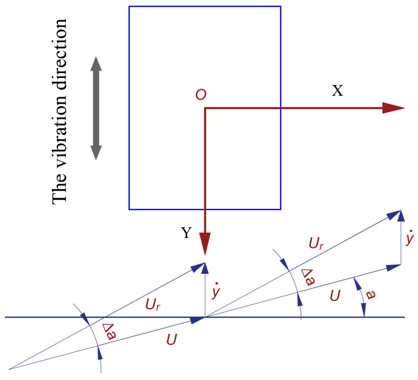
2.1. The Improved Method

In this section, a square section is taken as the research object. The structure has two main vibration axes: X and Y. Galloping generally occurs in conditions with a wind attack angle near 0° or 90°. When the wind attack angle is near 0°, the structure gallops in the Y direction; when the wind attack angle is around 90°, the galloping vibration of the structure is in the X direction, and the vibration direction is perpendicular to the main axis of the model. The research methods for these two cases are the same [21]. Therefore, this study chose the situation in which the wind attack angle is around 0°, and the vibration is in the Y direction. The parameter $\dot{y}$ is the speed in the vibration direction. When the wind attack angle with respect to the direction of vibration is α, due to the vibration of the structure, an additional relative wind attack angle ∆α is generated between the incoming flow and the structure, as shown in Figure 1.

According to the sine theorem, the following is obtained:

$$\frac{U_r}{\sin \left(90+\alpha \right)}=\frac{\dot{y}}{\sin \mathsf{\Delta }\alpha }$$

(1)

$$\sin △\alpha =\frac{\dot{y}}{U_r}\cos \alpha$$

(2)

According to the cosine theorem, the following is obtained:

$$U_r=\sqrt{{\left(\dot{y}\right)}^2+U^2+2U\dot{y}\sin \alpha }$$

(3)

Equation (2) is substituted into Equation (3), which yields

$$\sin △\alpha =\frac{\dot{y}\cos \alpha }{\sqrt{{\left(\dot{y}\right)}^2+U^2+2U\dot{y}\sin \alpha }}$$

(4)

$$△\alpha =\arcsin \frac{\dot{y}\cos \alpha }{\sqrt{{\left(\dot{y}\right)}^2+U^2+2U\dot{y}\sin \alpha }}$$

(5)

Considering that the vibrations are micro-vibrations, Equation (5) can be approximately expressed as

$$△\alpha \approx \frac{\dot{y}\cos \alpha }{\sqrt{{\left(\dot{y}\right)}^2+U^2+2U\dot{y}\sin \alpha }}$$

(6)

Under a uniform flow at an angle α, the force acting on the structure can be expressed as

$$F_y\left(\alpha \right)=-F_D\left(\alpha \right)\sin \alpha -F_L\left(\alpha \right)\cos \alpha$$

(7)

where F_D (α) and F_L (α) denote the drag force and the lift force under the wind axis coordinate system, respectively, which can be expressed as

$$F_D\left(\alpha \right)=\frac{1}{2}\rho U^{2}D{C}_D\left(\alpha \right)$$

(8)

$$F_L\left(\alpha \right)=\frac{1}{2}\rho U^{2}D{C}_L\left(\alpha \right)$$

(9)

where $\rho$ and D represent the air density, which is equal to 1.225 kg/m³, and the characteristic length of a column with a square cross section, respectively.

Equations (8) and (9) are substituted into Equation (7), which yields

$$F_y=\frac{1}{2}\rho U^{2}D\left(-C_D\left(\alpha \right)\sin \alpha -C_L\left(\alpha \right)\cos \alpha \right)$$

(10)

The derivative of F with respect to X can be expressed as

$$\frac{d{F}_y}{d\alpha }=-\frac{1}{2}\rho U^{2}D\left(\begin{array}{l}\cos \alpha C_D+\sin \alpha \frac{d{C}_D}{d\alpha }\\ -\sin \alpha C_L+\cos \alpha \frac{d{C}_L}{d\alpha }\end{array}\right)$$

(11)

The self-excited aerodynamic force generated by the addition of a relative wind angle $\mathsf{\Delta }\alpha$ can be expressed as

$$\begin{array}{cc}\hfill △F_y& =\frac{d{F}_y}{d\alpha }△\alpha \hfill \\ & =-\frac{1}{2}\rho U^{2}D\left(\begin{array}{l}\cos \alpha C_D+\sin \alpha \frac{d{C}_D}{d\alpha }\\ -\sin \alpha C_L+\cos \alpha \frac{d{C}_L}{d\alpha }\end{array}\right)△\alpha \hfill \end{array}$$

(12)

Equation (5) is substituted into Equation (12), which yields

$$△F_y=\frac{d{F}_y}{d\alpha }△\alpha =-\frac{1}{2}\rho U^{2}D\left(\begin{array}{l}\cos \alpha C_D+\sin \alpha \frac{d{C}_D}{d\alpha }\\ -\sin \alpha C_L+\cos \alpha \frac{d{C}_L}{d\alpha }\end{array}\right)\frac{\dot{y}\cos \alpha }{\sqrt{{\left(\dot{y}\right)}^2+U^2+2U\dot{y}\sin \alpha }}$$

(13)

The galloping force coefficient can be expressed as Q:

$$\begin{array}{cc}\hfill Q& =\cos \alpha C_D+\sin \alpha \frac{d{C}_D}{d\alpha }\hfill \\ & -\sin \alpha C_L+\cos \alpha \frac{d{C}_L}{d\alpha }\hfill \end{array}$$

(14)

when the section is axially symmetrical along the direction of vibration, the range of change in the wind attack angle can be regarded as −90° < α < 90°, and the galloping force coefficient can only be calculated in this range.

In Equation (13), when −90° < α < 90°, $\cos \alpha >0$; when $Q\ge 0$, $\mathsf{\Delta }{F}_y$ is opposite to $\dot{y}$, and the self-excited aerodynamic force is negative. So, in the state of micro-vibration, the aerodynamic force causes the dissipation of energy in the structural system, and the vibration is limited. When $Q<0$, $\mathsf{\Delta }{F}_y$ and $\dot{y}$ have the same sign, and the self-excited aerodynamic force performs positive work and continuously inputs energy into the structural system. Then, the amplitude of the structure gradually increases, which causes the phenomenon of vibration divergence. From another point of view, when $Q\ge 0$, positive aerodynamic damping is generated, which means that the total damping of the system is positive, and galloping instability does not occur in the structure. When $Q<0$, negative aerodynamic damping occurs, but the negative damping needs to be greater than the structure’s own damping to cause galloping instability. Therefore, $Q<0$ is a necessary condition for judging the galloping instability. Therefore, $\cos \alpha C_D+\sin \alpha \frac{d{C}_D}{d\alpha }-\sin \alpha C_L+\cos \alpha \frac{d{C}_L}{d\alpha }$ is the criterion for quasi-steady galloping stability.

Accordingly, the differential equation of motion can be expressed as follows:

$$m\left(\ddot{y}+2\zeta \omega \dot{y}+{\omega }^{2}y\right)=-\frac{1}{2}\rho U^{2}D\left(\begin{array}{l}\cos \alpha C_D+\sin \alpha \frac{d{C}_D}{d\alpha }\\ -\sin \alpha C_L+\cos \alpha \frac{d{C}_L}{d\alpha }\end{array}\right)\frac{\dot{y}\cos \alpha }{\sqrt{{\left(\dot{y}\right)}^2+U^2+2U\dot{y}\sin \alpha }}$$

(15)

where ζ, ω, and m denote the damping ratio, circular frequency of vibration, and mass of the model, respectively.

In the static flow field around the section of the bluff body, the relationship among the lift coefficient in the wind axis coordinate system, the drag coefficient in the wind axis coordinate system, and the lift coefficient in the body axis coordinate system can be expressed as

$$C_V=\cos \alpha C_L+\sin \alpha C_D$$

(16)

The derivative of C_V with respect to α in Equation (16) can be expressed as

$$\begin{array}{cc}\hfill \frac{d{C}_V}{d\alpha }& =\cos \alpha C_D+\sin \alpha \frac{d{C}_D}{d\alpha }\hfill \\ & -\sin \alpha C_L+\cos \alpha \frac{d{C}_L}{d\alpha }\hfill \end{array}$$

(17)

It can be deduced from Equation (17) that the value of dC_V/dα is equivalent to the value of Q. The criterion in Equation (14) can be further expressed as

$$\frac{d{C}_V}{d\alpha }=Q$$

(18)

Accordingly, the differential equation of motion can be rewritten as

$$m\left(\ddot{y}+2\zeta \omega \dot{y}+{\omega }^{2}y\right)=-\frac{1}{2}\rho U^{2}D\frac{d{C}_V}{d\alpha }$$

(19)

Then, the damping of the system can be expressed as

$$d=2m\zeta \omega +\frac{1}{2}\rho UD\frac{d{C}_V}{d\alpha }$$

(20)

when $d=0$, the critical wind speed for galloping at a wind attack angle of $\alpha$ can be expressed as

$$U_{cg}=\frac{-4m\zeta \omega }{\rho D\frac{d{C}_V}{d\alpha }}$$

(21)

where C_V is equal to the statistical average value of the lift coefficient on the body axis in a steady flow field, which can be calculated through wind tunnel tests or computational fluid dynamics (CFD) simulations.

The meaning of replacing $\cos \alpha C_D+\sin \alpha \frac{d{C}_D}{d\alpha }-\sin \alpha C_L+\cos \alpha \frac{d{C}_L}{d\alpha }$ with $\frac{d{C}_V}{d\alpha }$ is that the possibility of quasi-steady galloping can be directly judged by observing the trend of change in the parameter C_V at every wind attack angle $\alpha$. When dC_V/dα < 0, the structure may gallop, and the galloping stability should be analyzed on the bridge. When dC_V/dα > 0, the structure does not gallop. In theory, the calculation result of Equation (17) is consistent with that of dC_V/dα, but inevitable errors often occur during data processing, as there are too many parameters in Equation (17), leading to a relatively large error between the two equations. Therefore, the calculation process for dC_V/dα is concise enough to improve the calculation accuracy.

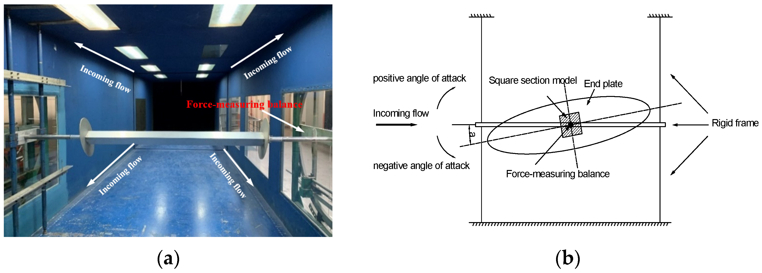
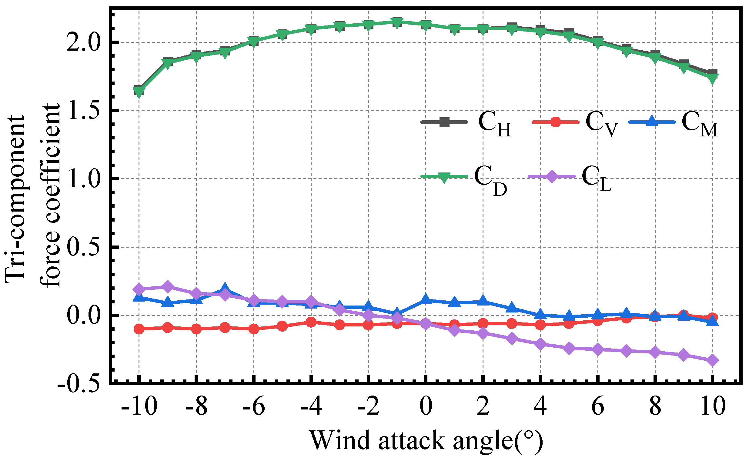
2.2. Wind Tunnel Tests

A tri-component force test of a square-section model that could experience quasi-steady galloping at highly reduced wind speeds was carried out in the CA-1 atmospheric boundary layer wind tunnel of the Chang’an University Wind Tunnel Laboratory, which is shown in Figure 2. The dimensions of the test section were 15 m (length) × 3.0 m (width) × 2.5 m (height), with an adjustable wind velocity range of 0.2–53 m/s. The transverse characteristic dimension D of the test model was 0.14 m, and the model’s length L was 1.8 m. The square-section model was directly fixed in the wind tunnel with stiff poles. The end parts of the model were directly installed on a force-measuring balance, and the wind attack angle ranged from −10° to 10°, resulting in a total of 21 working conditions.

The curves of the static tri-component force coefficient of the body axis and the wind axis coordinate systems at every wind attack angle are shown in Figure 3.

2.3. Theoretical Solution

Xie introduced the equivalent wind attack angle and equivalent wind speed into the structural vibration equation according to their geometric relationship and expanded the equivalent wind attack angle into a linear expression of the structure’s transverse wind direction vibration velocity $\dot{y}$. The critical wind speed of galloping in the wind axis coordinate system can be expressed as

$$U_{cg-x}=\frac{-4m\zeta \omega }{\rho D\left[\left(\frac{d{C}_D}{d\alpha }+C_L\right)\sin \alpha \cos \alpha +\frac{d{C}_L}{d\alpha }{\cos }^2\alpha +C_D{\sin }^2\alpha +C_D\right]}$$

(22)

At the same time, Xie et al. derived the formula for calculating the galloping amplitude based on the galloping force coefficient with the wind’s angle of attack. The calculation results were in good agreement with the test results, which proved the accuracy of the calculation.

The classic Den Hartog criterion, the dC_V/dα criterion, and the Xie criterion all contain the derivative of the tri-component force coefficient; so, it was necessary to fit the tri-component force coefficient curve shown in Figure 3. However, if the value of the tri-component force coefficient was small, the reliability of the fitted curve would have a great impact on its derivative. To reduce the error, the thir-order, fourth-order, fifth-order, and ninth-order nonlinear polynomial fitting curves of each tri-component force coefficient curve were plotted. Then, the original broken line and each fitting curve were derived. For example, the derivative curve of the lift coefficient C_L in the wind axis coordinate system is shown in Figure 4, and the correlation coefficients are shown in

Table 1. Correlation coefficients.

Modality	Pearson	Spearman	Kendall
Third order	0.92737	0.97464	0.90389
Fourth order	0.95118	0.97464	0.90389
Fifth order	0.96341	0.97464	0.90389
Ninth order	0.94683	0.98699	0.93978

. The fitted derivative curve with the highest correlation coefficient was selected for the subsequent calculations with the aforementioned formula.

By substituting the tri-component force coefficients that were processed above into the Den Hartog criterion, the dC_V/dα criterion, and the criterion proposed by Xie Lambo, the galloping force coefficients were calculated and are shown in Figure 5. It could be deduced that the galloping force coefficients of the three criteria were almost the same in the range of smaller wind attack angles. As the absolute value of the wind attack angle increased, the error between the calculation results of the dC_V/dα criterion and the Den Hartog criterion also gradually increased, indicating that the dC_V/dα criterion had enough reliability in the range of small wind attack angles. At a larger absolute value of the wind attack angle, the Den Hartog criterion was no longer applicable, thus showing the necessity of considering the influence of the wind attack angle on the galloping force coefficient.

3. Verification of the Critical Wind Speed of Galloping

To further verify the reliability and effectiveness of the improved standard proposed in this study at high angles of attack, in this section, an H-shaped section is taken as the research object. This section also describes the wind tunnel tests that were conducted and compares the critical wind speed of galloping calculated according to Formula (21) with the measured critical speed of galloping.

3.1. Force and Vibration Tests on an H-Type Hanger-Section Model

The wind tunnel test on the H-shaped-section model is shown in Figure 6a. According to the test requirements from the “Code for Design of Wind Resistance of Highway Bridges and Culverts” (JTG/T 3360-01-2018), galloping tests should be carried out in a uniform flow field, and the incoming flow angle of attack should be from 0° to 90° in increments of 5°. The specific section parameters and wind attack angles are shown in Figure 6b.

The measured vertical bending frequency was 4.55 Hz, and the damping ratio of the model was 0.583%. The incoming wind speed was 13 m/s. The measured curves of the tri-component force coefficient in the uniform flow field are shown in Figure 7.

3.2. Comparison and Analysis of the Theoretical Results

The measured tri-component force coefficients shown in Figure 7 were processed according to the method described in the section on the theoretical solution. Then, the galloping force coefficients, which are shown in Figure 8, were calculated with Equation (18) and the Den Hartog criterion with the processed data. It can be seen in Figure 8 that with wind attack angles within the range of 0°–5°, the values of the galloping force coefficient calculated with the dC_V/dα criterion and the Den Hartog criterion were very close. With wind attack angles within the range of 5°–25°, the error of the galloping force coefficients calculated with the two criteria gradually increased, but it was still relatively small. When the wind attack angle was larger than 25°, the galloping force coefficients obtained with the Den Hartog criterion were all greater than those obtained with the dC_V/dα criterion, and the difference was huge, which is consistent with the conclusions obtained in the section on the theoretical solution.

Considering that the curve of the measured tri-component force coefficient contained discrete data with increases of 5°, errors could easily occur in the curve-fitting and derivation process, which would distort the calculation results. Therefore, the calculated galloping force coefficient under working conditions of 70°, which had a relatively small difference, was selected to calculate the critical wind speed of galloping. Then, the calculated critical wind speed of galloping was compared with the measured critical wind speed of galloping. The wind speed–displacement curve at a wind attack angle of 70° is shown in Figure 9.

According to the results in

Table 2. Comparison of critical wind speeds of galloping.

	Den Hartog	(dCV)/dα	Measured
Critical Wind Speed of Galloping	16.134	10.200	11.204
Absolute Error	4.930	−1.004	—

, the (dC_V)/dα method had a small error between the calculated critical wind speed of galloping and the measured critical wind speed at large angles of attack, and the result was more conservative, which could prove the validity and reliability of the (dC_V)/dα criterion. In addition, to improve the calculation accuracy and make the calculation results more reliable, the amplitude of the variations in the wind attack angle should be reduced. For example, a force measurement test was performed for every additional 1° in the wind attack angle, and enough samples of the tri-component force coefficient were collected in the wind tunnel tests to ensure—to some extent—that the calculated parameters were not distorted during the curve-fitting and derivation process.

4. Numerical Simulation

To further study the flow characteristics of the flow field around the H-shaped section under the critical wind speed of galloping, the computational fluid dynamics software Fluent was used to carry out a numerical simulation of the H-shaped section.

4.1. Governing Equations and Discretization Methods

In this section, the Reynold-averaging method was used for a numerical simulation of turbulent motion, and the SST K-w turbulence model was used for the calculations [32]. The discretization of the fluid control equations was performed based on the finite volume method. The second-order upwind scheme was used for the convection term, and the semi-implicit SIMPLE method was used for the velocity–pressure coupling term.

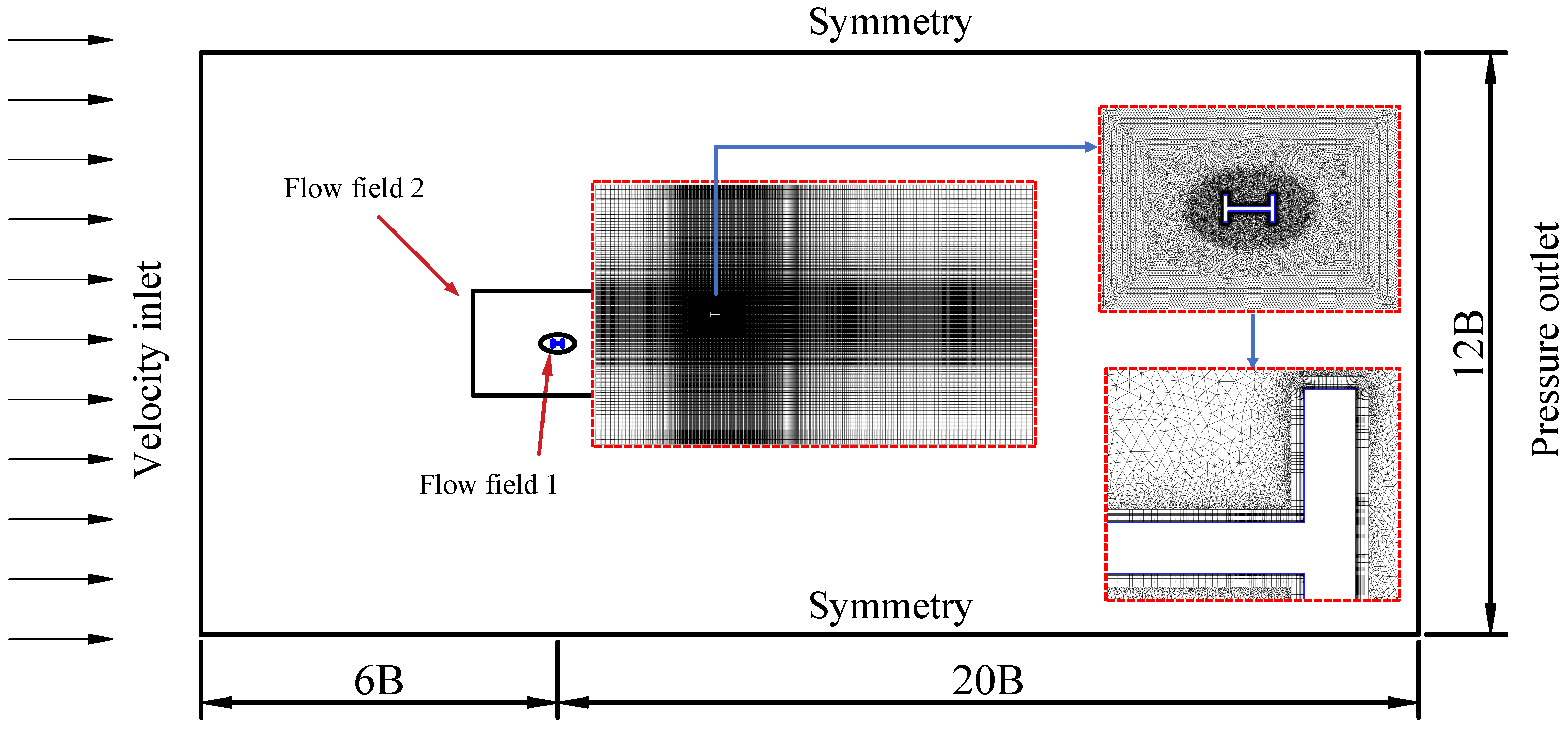
4.2. Computational Domain Mesh and Flow Condition Settings

The CFD numerical simulation used the same scale and incoming wind speed as those in the wind tunnel test. The calculation domain size settings are shown in Figure 10. The total size of the calculation field was 26B long × 12B wide (B is the section width) with a turbulence intensity of I_u = 0.5%, which met the requirements of the model blocking ratio (<5%).

At the same time, to accurately simulate the separation and transition of flow near the wall and meet the requirements of y⁺ < 1 in most areas around the section, the thickness of the first layer of the grid was 0.00005 m, and the grid growth rate was set to 1.1 from the inside to the outside.

Due to the large amount of vortex shedding in the wake region of the H-shaped section, to better capture the motion of the vortex in the wake region of the structure, the grid in the wake region needed to be properly densified [33]. A mixed grid (structured grid and unstructured grid) was used in flow field 1, a structured grid was used in flow field 2, and a structured grid was used in the other regions. The grid division and detailed structure are shown in Figure 10.

4.3. Independence Verification and Comparison of the Results

The quantity, quality, and time step of the grid had a great impact on the simulation results. In order to ensure the accuracy and effectiveness of the numerical simulation, it was necessary to check the independence of the grid and the time before the calculation. The grid inspection results are shown in

Table 3. Grids with different quantities and numerical results.

Grid	Total Cells	Total Nodes	Triangular Cells	Quadrilateral Cells	Cm	Cl	Cd
Mesh1	124,392	82,402	85,880	38,512	0.000036	0.000175	1.397378
Mesh2	151,394	95,993	112,882	38,512	0.000047	0.000152	1.403204
Mesh3	175,878	108,235	137,366	38,512	0.000041	0.000106	1.410183

.

The verification of grid independence and time independence is a necessary step when selecting the number of grids and time steps. After considering the length of the section and the inlet wind speed, three time steps were selected for the verification of the time independence. They were 5 × 10⁻³, 1 × 10⁻³, and 5 × 10⁻⁴. It was found that the deviation of the calculation results in the three time steps was within 1%. After considering the calculation efficiency and accuracy, the final selected grid number was 15.1 w, with a time step of 5 × 10⁻⁴.

4.4. Comparison of Numerical Simulation and Experimental Results

The comparison between the CFD simulation results and the experimental results is shown in Figure 11, and it can be seen that the simulation results were basically consistent with the experimental values. As for the errors, they were in part caused by the production and installation of the experimental model itself. In addition, the two–dimensional numerical simulation in this article could not truly simulate the airflow around the cross section in three–dimensional conditions, and these errors could be considered to be within a reasonable range. Therefore, it could be considered that the numerical simulation method used in this article was correct.

Figure 12 shows the vibration mode of the H-shaped section under the critical wind speed of a galloping vibration. It can be seen that there was a significant unsteady vibration on the H-shaped section at this wind speed. The main frequency of the vibration displacement mode was 4.31 Hz, which is basically consistent with the main frequency of 4.2 Hz in the aerodynamic force of the section. At the same time, it was very close to the vertical vibration frequency of 4.55 H_Z of the H-shaped section itself, which further illustrates the correctness of the simulation method used in this paper. In addition to the main frequency, there were other modal frequency components present in the aerodynamic force of this section. However, among these modes, the first-order mode contained the highest energy, indicating that the dominant mode of the H-shaped section was 4.2 Hz.

4.5. Results of the Numerical Simulations

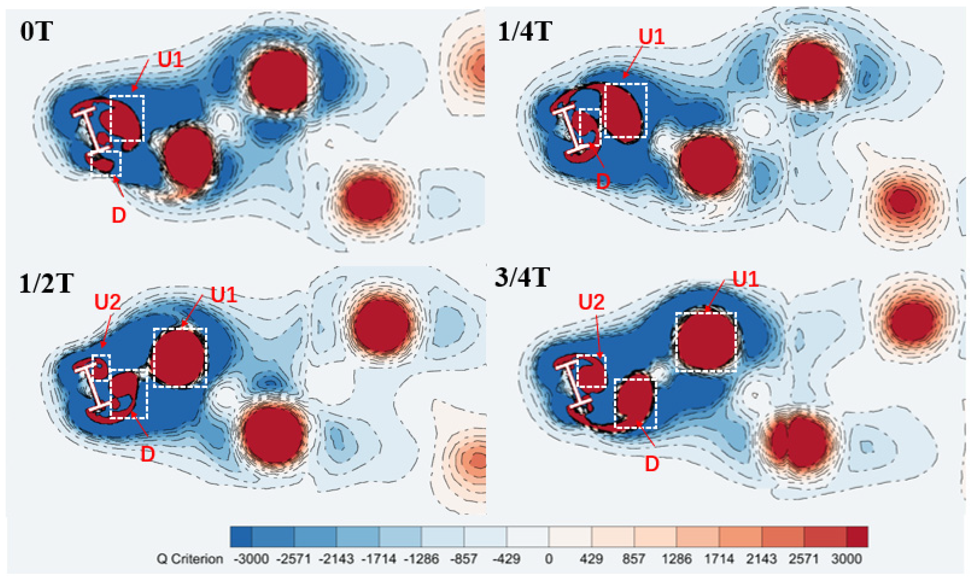
4.5.1. Characteristics of the Evolution of Vorticity around the H-Shaped Section

The evolution of vorticity around the section over a period under the critical wind speed of galloping was obtained in the CFD numerical simulation, as shown in Figure 13. In this section, the Q criterion was used to identify vorticity. When Q > 0, the rotation rate is greater than the strain rate, and this area is represented as a vortex (red part in the figure). When Q < 0, the rotation rate is less than the strain rate, and the motion of the fluid unit is non-rotating (blue area in the figure).

In Figure 13, it can be seen that there was a pair of obvious and large vortex structures in the wake region of the H-shaped cross-section at a wind attack angle of 70°. The vortex located on the upper side of the section was named U, and the vortex located on the lower side of the section was named D. In the initial stage, when the airflow passed through the upper edge of the H-shaped section, it first caused airflow separation and generated a vortex structure (U1). At the same time, a small vortex structure (D) developed at the lower edge of the H-shaped section. During the T/4 period, the vortex (U1) developed in the main vortex and gradually began to detach from the H-shaped cross section. At this time, the vortex structure (D) below the cross section gradually developed and became larger. In the T/2 period, the vortex U1 generated on the upper surface had already separated from the cross section, and the lower vortex (D) had become the main vortex structure of the H-shaped cross section, occupying the dominant position. At the same time, a new vortex structure (U2) was generated at the upper edge of the H-shaped section, and the vortex gradually developed, separated, and detached. It can be seen that during a cycle, when the airflow passed through the H-shaped section, vortex separation and shedding phenomena continuously occurred in the wake area of the section, which caused periodic forces on it, leading to the aerodynamic instability of the H-shaped section.

4.5.2. Trace Diagram of the Flow Field around the Section

In order to more clearly show the characteristics of the changes in the flow field around the H-shaped section, a flow trace diagram around the H-shaped section was drawn, as shown in Figure 14.

It can be seen in the Figure that there were obviously different vortex structures in the wake region of the H-shaped section. In the beginning, there were three typical vortex structures (M1, M2, and M3) in the wake region of the section. As time went on, the vortex gradually moved backward, and the M3 vortex gradually developed from small to large. In the T/2 stage, a new vortex structure (M4) appeared at the lower edge of the H-shaped section. With the vortex M3 moving backward from the structure, M4 developed into the main vortex of the section. As a result, alternating vortices were continuously formed in the wake region of the H-shaped section, which caused the vibration of the structure.

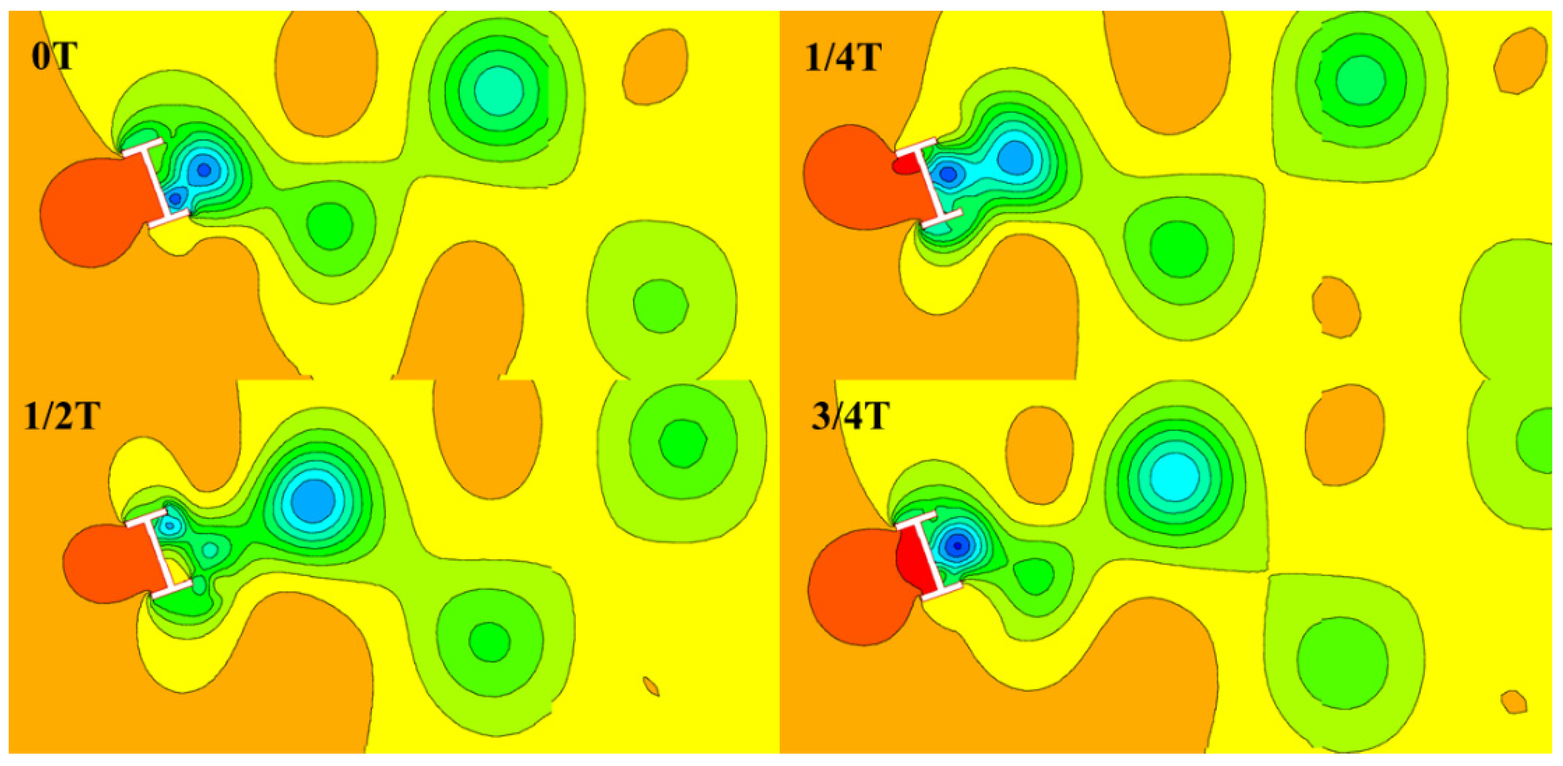
4.5.3. Pressure Distribution around the H-Shaped Section

Figure 15 shows the distribution characteristics of low pressure in the separation area around the H-shaped section. It can be clearly seen that due to the influence of incoming airflow, the windward side of the H-shaped section was in a significant positive pressure area, while there was a significant negative pressure area in the area of the leeward side, and the position of this negative pressure area constantly changed with the motion of the vortex. Within a range of time, the center position of the negative pressure zone also constantly moved up and down. This central change in the negative pressure zone caused the section to undergo a periodic force, which caused the H-shaped section to generate a galloping phenomenon. It was proved again that aerodynamic instability would occur in the H-shaped section at this wind speed.

5. Conclusions

In this study, the Den Hartog’s classical method of calculating the quasi–steady critical wind speed of galloping was studied. By taking a square column section as the target and through theoretical analysis, a correction method for the galloping force coefficient that considered the influence of the wind attack angle is proposed. A wind tunnel test was carried out to verify this method with an H-shaped section. At the same time, the flow around the section at the critical wind speed of galloping was studied with a numerical simulation. The research results are as follows:

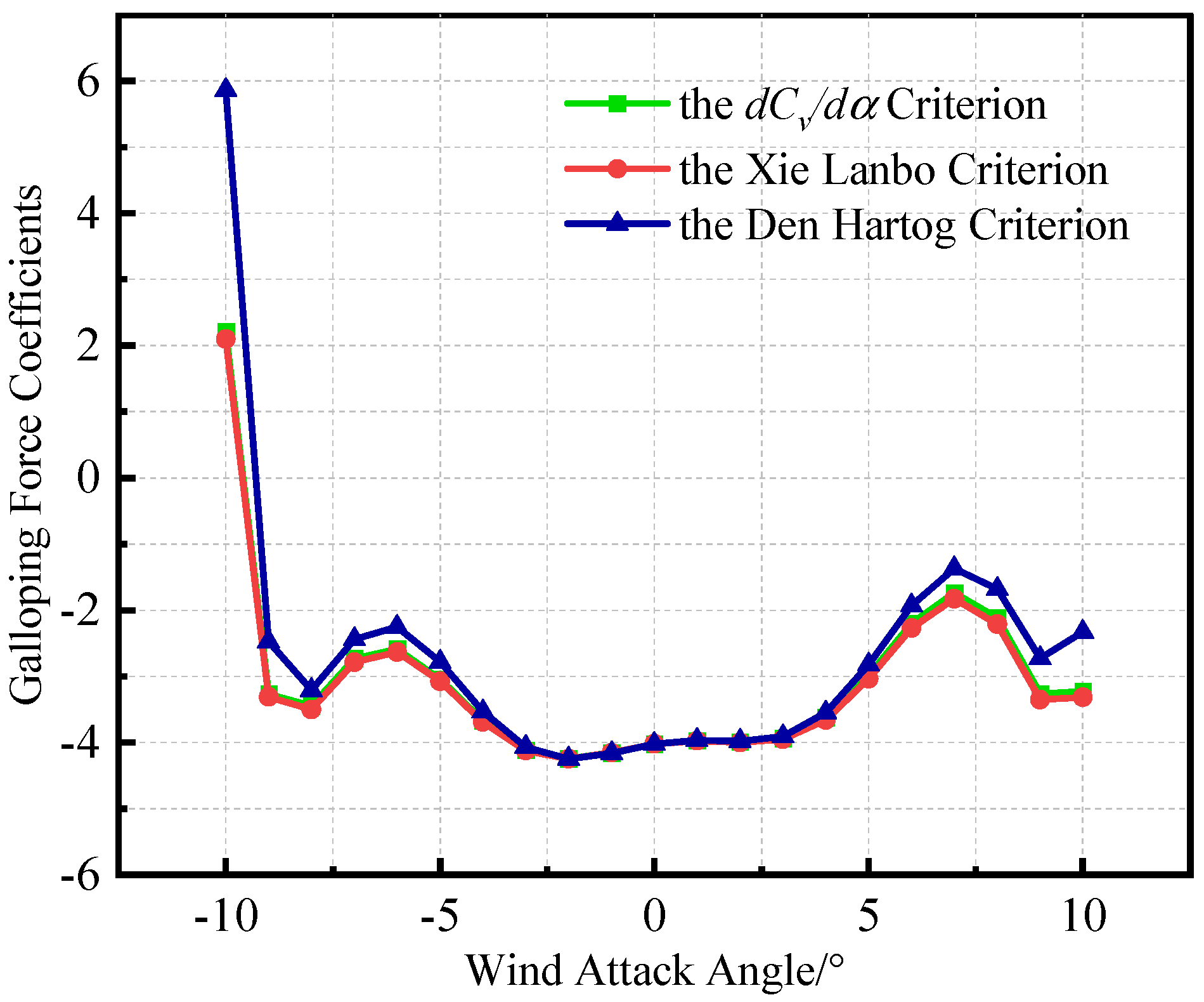
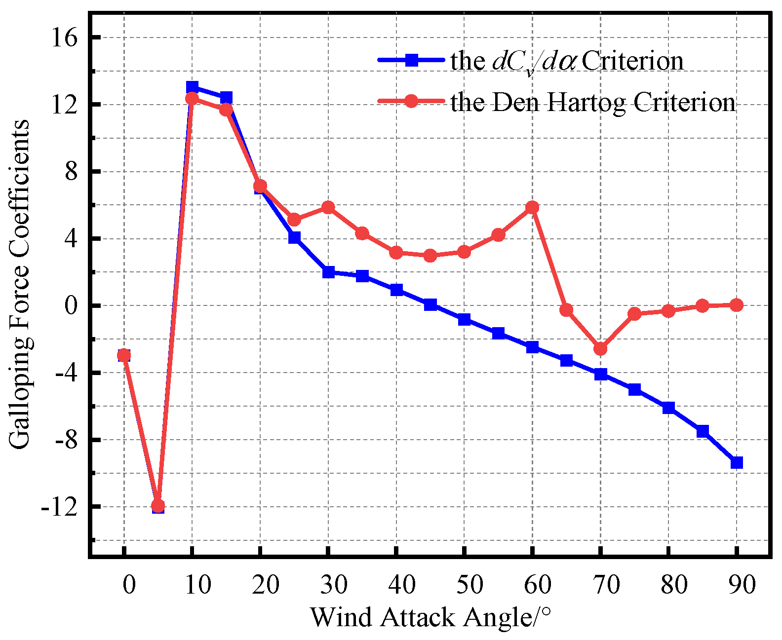
• Compared with the classical Den Hartog calculation method and the method proposed by Xie, this study proposes a modified judgment criterion for the galloping force coefficient that considers the impact of the wind attack angle. In the range of wind attack angles of less than 25°, the calculation results were basically consistent. The correction method proposed in this study was better than the classical calculation method based on the Den Hartog criterion, which did not consider the influence of the wind attack angle.
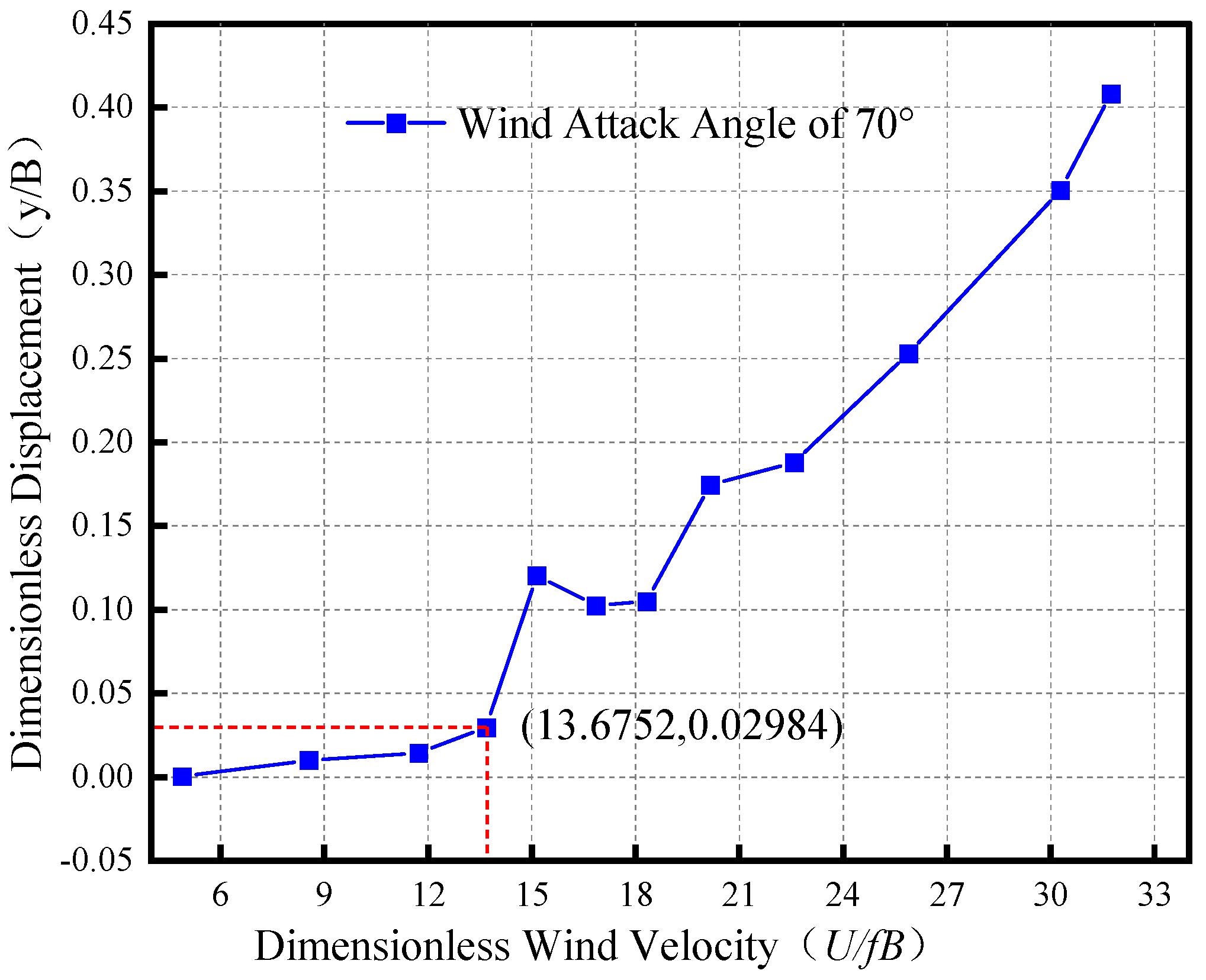
• To further verify the applicability of this method, a model wind tunnel test was conducted on an H-shaped section at a high angle of attack. It was found that the critical wind speed of galloping calculated with the method that considered the wind’s angle of attack was 10.2 m/s, which was closer to the critical wind speed of 11.2 m/s measured in the wind tunnel.
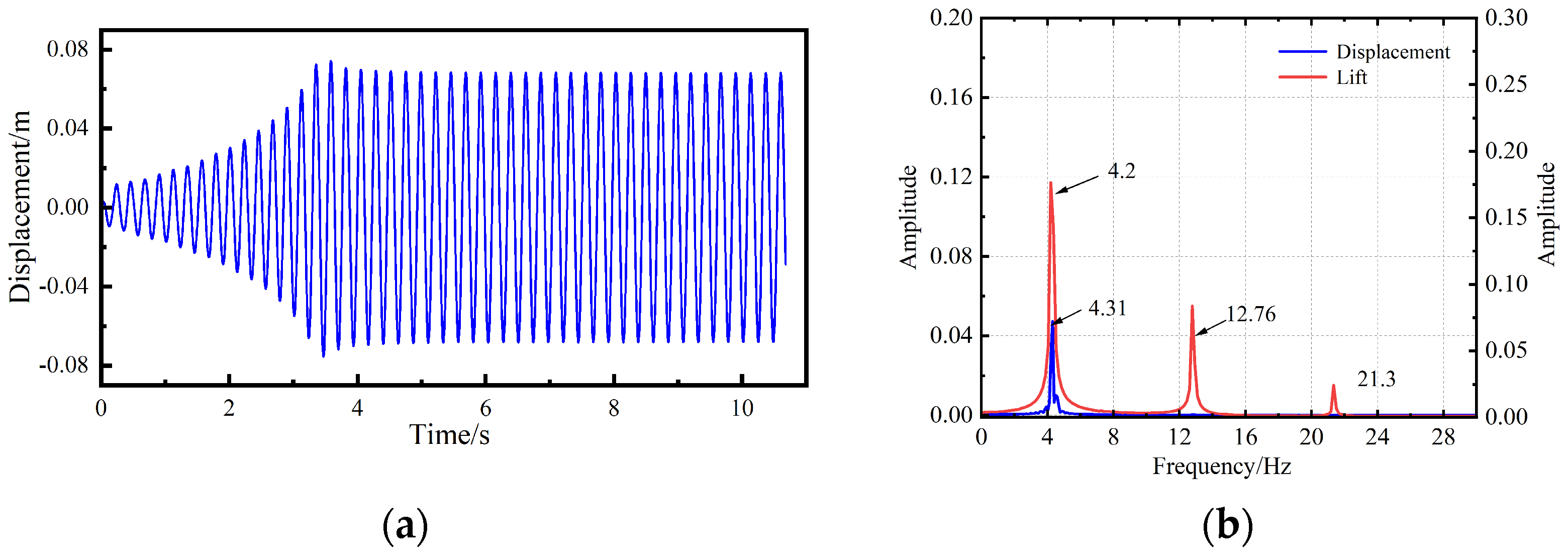
• The results of the numerical simulation showed that at the critical wind speed of galloping, there was obvious airflow separation around the H-shaped section, and a large number of vortices fell off at the tail edge of the section, resulting in the instability of the section, which further verified the existence of severe aerodynamic instability at this wind speed.

References

1. Parkinson, G.V. Wind-induced Instability of Structures. Philos. Trans. R. Soc. 1971, 269, 395–409. [Google Scholar]
2. Païdoussis, M.P.; Price, S.J.; De Langre, E. Fluid-Structure Interactions: Cross-Flow-Induced Instabilities; Cambridge University Press: Cambridge, UK, 2010. [Google Scholar]
3. Robertson, I.; Li, L.; Sherwin, S.; Bearman, P. A numerical study of rotational and transverse galloping rectangular bodies. J. Fluids Struct. 2003, 17, 681–699. [Google Scholar] [CrossRef]
4. Alonso, G.; Meseguer, J.; Pérez-Grande, I. Galloping instabilities of two-dimensional triangular cross-section bodies. Exp. Fluids 2005, 38, 789–795. [Google Scholar] [CrossRef]
5. Alonso, G.; Meseguer, J.; Pérez-Grande, I. Galloping stability of triangular cross-sectional bodies: A systematic approach. J. Wind Eng. Ind. Aerodyn. 2007, 95, 928–940. [Google Scholar] [CrossRef]
6. Alonso, G.; Sanz-Lobera, A.; Meseguer, J. Hysteresis phenomena in transverse galloping of triangular cross-section bodies. J. Fluids Struct. 2012, 33, 243–251. [Google Scholar] [CrossRef]
7. Barrero-Gil, A.; Sanz-Andrés, A.; Alonso, G. Hysteresis in transverse galloping: The role of the inflection points. J. Fluids Struct. 2009, 25, 1007–1020. [Google Scholar] [CrossRef]
8. Abdelkefi, A.; Hajj, M.R.; Nayfeh, A.H. Piezoelectric energy harvesting from transverse galloping of bluff bodies. Smart Mater. Struct. 2012, 22, 015014. [Google Scholar] [CrossRef]
9. Shoshani, O. Theoretical aspects of transverse galloping. Nonlinear Dyn. 2018, 94, 2685–2696. [Google Scholar] [CrossRef]
10. Regev, S.; Shoshani, O. Investigation of transverse galloping in the presence of structural nonlinearities: Theory and experiment. Nonlinear Dyn. 2020, 102, 1197–1207. [Google Scholar] [CrossRef]
11. Bearman, P.W.; Luo, S.C. Investigation of the aerodynamic instability of a square-section cylinder by forced oscillation. J. Fluids Struct. 1988, 2, 161–176. [Google Scholar] [CrossRef]
12. Nakamura, Y.; Matsukawa, T. Vortex excitation of rectangular cylinders with a long side normal to the flow. J. Fluid Mech. 1987, 180, 171–191. [Google Scholar] [CrossRef]
13. Obasaju, E.D. An investigation of the effects of incidence on the flow around a square section cylinder. Aeronaut. Q. 1983, 34, 243–259. [Google Scholar] [CrossRef]
14. Niu, H.; Zhou, S.; Chen, Z.; Hua, X. An empirical model for amplitude prediction on VIV-galloping instability of rectangular cylinders. Wind Struct. 2015, 21, 85–103. [Google Scholar] [CrossRef]
15. Chen, Z.Q.; Liu, M.G.; Hua, X.G.; Mou, T. Flutter, galloping, and vortex-induced vibrations of H-section hangers. J. Bridge Eng. 2012, 17, 500–508. [Google Scholar] [CrossRef]
16. Bai, H.; Li, R.; Guo, C.M.; Li, J.W.; Zhang, Y.J. Optimization of aerodynamic performance of H-section hangers. J. Vib. Shock 2020, 39, 186–193. [Google Scholar]
17. Ma, T.F. Influence of Mass and Damping Parameters and Turbulence on Galloping and Vortex-Induced Vibration of H-Shape Hanger. Master’s Thesis, Chang’an University, Xi’an, China, 2019. [Google Scholar]
18. Xie, L.B. Study on the Nonlinear Self-Excited Aerodynamic Force and Galloping Characteristics of H-Shaped Cross Section Structures. Master’s Thesis, Southwest Jiaotong University, Chengdu, China, 2016. [Google Scholar]
19. Gao, G.; Zhu, L. Measurement and verification of unsteady galloping force on a rectangular 2: 1 cylinder. J. Wind Eng. Ind. Aerodyn. 2016, 157, 76–94. [Google Scholar] [CrossRef]
20. Gao, G.; Zhu, L. Nonlinear mathematical model of unsteady galloping force on a rectangular 2: 1 cylinder. J. Fluids Struct. 2017, 70, 47–71. [Google Scholar] [CrossRef]
21. Mannini, C.; Massai, T.; Marra, A.M. Modeling the interference of vortex-induced vibration and galloping for a slender rectangular prism. J. Sound Vib. 2018, 419, 493–509. [Google Scholar] [CrossRef]
22. Chen, C.; Mannini, C.; Bartoli, G.; Thiele, K. Experimental study and mathematical modeling on the unsteady galloping of a bridge deck with open cross section. J. Wind Eng. Ind. Aerodyn. 2020, 203, 104170. [Google Scholar] [CrossRef]
23. Tang, H.J.; Li, Y.L.; Liao, H.L. Energy method of galloping analysis for 2D square cylinder. J. Basic Sci. Energy 2015, 23, 104–114. [Google Scholar]
24. Chen, K. Experimental study on galloping characteristic and improvement measure for single column tower by wind tunnel test. Railw. Eng. 2017, 57, 34–35. [Google Scholar]
25. Yan, Z.C.; Yang, J.X.; Ni, Z.J.; Wu, R.H.; Zhang, L.L. Research on galloping vibration of cable-stayed bridge with single-column tower and variable cross-section. Highway 2020, 65, 207–211. [Google Scholar]
26. Li, S.Y.; Wu, T.; Huang, T. Aerodynamic stability of iced stay cables on cable-stayed bridge. Wind Struct. 2016, 23, 253–273. [Google Scholar] [CrossRef]
27. Li, S.Y.; Zheng, Q.Y.; Wen, X.G.; Chen, Z. Numerical simulations and tests for dry galloping mechanism of stay cables. J. Vib. Shock 2017, 36, 100–105. [Google Scholar]
28. Ma, W.Y.; Yuan, X.X.; Wei, Y.Y.; Liu, Q.K. Effect of Reynolds number on aerodynamic force on and galloping instability of a cylinder with elliptical cross-section. J. Vib. Eng. 2016, 29, 730–736. [Google Scholar] [CrossRef]
29. Ma, W.Y.; Zhang, L.; Zhang, X.B.; Deng, R.R. Effect of yaw angle on the galloping instability of slender square structures. J. Vib. Shock 2021, 40, 171–175+184. [Google Scholar]
30. Xie, L.B.; Liao, H.L. Galloping calculation method for prisms with attack angle. J. Vib. Shock 2018, 37, 9–15+24. [Google Scholar]
31. Tang, H.J. Wind-Induced Vibration and Aerodynamic Measures of Long-Span Suspension Bridges with Steel Truss Girder in Complex Mountainous Canyon. Ph.D. Thesis, Southwest Jiaotong University, Chengdu, China, 2016. [Google Scholar]
32. Menter, F.R. Two-equation eddy-viscosity turbulence models for engineering applications. AIAA J. 1994, 32, 1598–1605. [Google Scholar] [CrossRef]
33. Mannini, C.; Šoda, A.; Schewe, G. Unsteady RANS modelling of flow past a rectangular cylinder: Investigation of Reynolds number effects. Comput. Fluids 2010, 39, 1609–1624. [Google Scholar] [CrossRef]
Figure 1. Diagram of the additional wind attack angle.
Applsci 13 05390 g001
Figure 2. The square-section model for the force test: (a) wind tunnel test; (b) schematic diagram of the segment model.
Applsci 13 05390 g002
Figure 3. Tri-component force coefficients of the square section with the wind axis and body axis coordinates.
Applsci 13 05390 g003
Figure 4. The derivative curves of the lift coefficient CL.
Applsci 13 05390 g004
Figure 5. Galloping force coefficients.
Applsci 13 05390 g005
Figure 6. H-shaped section: (a) wind tunnel test on the segment model; (b) parameters of the cross section and direction of the wind attack angle.
Applsci 13 05390 g006
Figure 7. Tri-component force coefficients.
Applsci 13 05390 g007
Figure 8. Galloping force coefficients.
Applsci 13 05390 g008
Figure 9. Wind speed–displacement curve.
Applsci 13 05390 g009
Figure 10. Division of the calculation domain and relevant grid diagram in the numerical simulation.
Applsci 13 05390 g010
Figure 11. Comparison results: (a) drag results; (b) lift results.
Applsci 13 05390 g011
Figure 12. Analysis of the vibration results: (a) vertical displacement; (b) amplitude spectrum.
Applsci 13 05390 g012
Figure 13. Diagram of the instantaneous evolution of vorticity in the H-shaped section (the wind attack angle was 70°).
Applsci 13 05390 g013
Figure 14. Flow trace diagram of the H-shaped cross section.
Applsci 13 05390 g014
Figure 15. Pressure distribution around the H-shaped section.
Applsci 13 05390 g015