Abstract
To achieve high-precision forecasting of different grades of albacore fishing grounds in the South Pacific Ocean, we used albacore fishing data and marine environmental factors data from 2009 to 2019 as data sources. An ensemble learning model (ELM) for albacore fishing grounds forecasting was constructed based on six machine learning algorithms. The overall accuracy (ACC), fishing ground forecast precision (P) and recall (R) were used as model accuracy evaluation metrics, to compare and analyze the accuracy of different machine learning algorithms for fishing grounds forecasting. We also explored the forecasting capability of the ELM for different grades of fishing grounds. A quantitative evaluation of the effects of different marine environmental factors on the forecast accuracy of albacore tuna fisheries was conducted. The results of this study showed the following: (1) The ELM achieved high accuracy forecasts of albacore fishing grounds (ACC = 86.92%), with an overall improvement of 4.39~19.48% over the machine learning models. (2) A better forecast accuracy (R2 of 81.82–98%) for high-yield albacore fishing grounds and a poorer forecast accuracy (R1 of 47.37–96.15%) for low-yield fishing grounds were obtained for different months based on the ELM; the high-yield fishing grounds were distributed in the sea south of 10° S. (3) A feature importance analysis based on RF found that latitude (Lat) had the greatest influence on the forecast accuracy of albacore tuna fishing grounds of different grades from February to December (0.377), and Chl-a had the greatest influence on the forecast accuracy of albacore tuna fishing grounds of different grades in January (0.295), while longitude (Lon) had the smallest effect on the forecast of different grades of fishing grounds (0.037).
1. Introduction
The albacore is a species of tuna of great economic relevance in the Pacific, Indian and Atlantic Oceans, as well as in other minor basins [1,2]. In recent years, with albacore becoming an important target of longline fisheries, the South Pacific has become one of the critical fishing areas for albacore globally [1,3]. With the development of China’s pelagic longline fishery, the rational exploitation and sustainable development of the pelagic fishery are of paramount importance [4,5]. Therefore, it has become a popular research topic to accurately forecast the distribution of different grades of albacore fishing grounds in the South Pacific Ocean and improve the accuracy of fishing forecasts and the fishing efficiency of fishermen.
In recent years, traditional models and machine learning algorithms have become important methods for fishing grounds forecasting [6,7,8,9]. For example, Chang et al. (2012) constructed the Habitat Suitability Index (HSI) model, which has become a reliable tool for forecasting potential fishing grounds of swordfish in the South Atlantic [10]. Fishing ground forecasts have shifted from small-scale and short-term fishery data to large-scale fishery data. Traditional models are limited by the dimensionality of the input data, which makes it challenging to achieve high-accuracy fishing ground forecasts for large-scale, complex and variable high-dimensional ocean data [11,12]. At the same time, traditional models also have problems, such as being influenced by human factors, not having generalizability, having difficulty in feature conversion and experiencing insufficient fitting [13,14]. Machine learning algorithms have effectively suppressed these problems in many classification and regression studies [15,16]. However, in the modeling process, it is difficult for machine learning models to achieve high-accuracy forecasting of the distribution of different grades of fishing grounds due to the complexity and variability of marine environmental factors and the limitations of single-model algorithms, such as poor stability, easy overfitting and poor generalization ability [17,18,19]. While ensemble learning can effectively solve these problems [20,21], ensemble learning algorithms produce more stable results by integrating the advantages of multiple base models and using multiple learners to solve problems together, which can effectively suppress model overfitting and improve model prediction [22,23,24,25]. For example, Dong et al. (2020) selected seven different machine learning algorithms for integrated learning to predict the habitat suitability of Hemiculter leucisculus and concluded that the ensemble model had the highest predictive power (AUC = 0.972) [26]. Rahman et al. (2021) conducted a polling integration based on three single models, and their study concluded that it outperformed a single machine learning model (R2 = 0.75) in predicting Malaysian marine fish production [9]. However, the application effect of the ensemble learning model on different grades of albacore fishing grounds in the South Pacific has not been verified.
The external environmental factors of marine fish survival are the main factors affecting the abundance and distribution of fishery resources [27,28]. It has been proved that the spatial and temporal distribution of fishing grounds, the living habits of marine fishes and marine environmental factors are very closely related [29,30]. Chen et al. (2005) verified the relationship between marine environmental factors and the distribution of albacore fishing grounds in the Indian Ocean, and the results showed that SST, Chl-a and SSS had significant effects on the distribution of immature albacore, with SST having a particularly prominent effect on the distribution of mature albacore fishing grounds [31]. Zainuddin et al. (2008) analyzed the relationship between albacore fishing grounds in the western North Pacific Ocean and sea surface height anomaly (SSHA), SST and Chl-a, and showed that the optimal range corresponding to the highest catch per unit effort (CPUE) was 18.5~21.5 °C for SST, 0.2~0.4 mg m−3 for Chl-a and −5.0~32.2 cm for SSHA [32]. However, due to the complexity of the marine environment itself, there are differences in the habitat environment of fish in different seas [33]. Daqamseh et al. (2019) showed that Chl-a was the most important marine environmental factor affecting the potential habitat of fish in the Saudi Arabian Red Sea, and the number of potential fishing zones (PFZs) was positively correlated with Chl-a and negatively correlated with SST and SSS [34]. Mondal et al. (2021) showed that SST and Chl-a influence the distribution of marine fish resources [35]. Therefore, a quantitative assessment of the influence of marine environmental factors on the forecast accuracy of South Pacific albacore fishing grounds based on RF feature importance analysis is particularly critical to achieve efficient fishing of South Pacific albacore.
To make up for the above research deficiencies, this paper took the South Pacific waters as the research area and constructed an albacore fishing grounds forecasting model based on the ensemble learning of five machine learning algorithms, namely, RF, SVM, KNN, XGBoost and GP, to realize the high-accuracy forecasting of different grades of albacore fishing grounds in the South Pacific. The main objectives were as follows: (1) to compare the forecast accuracy of different machine learning algorithms and the ELM for different grades of South Pacific albacore fishing grounds; (2) to explore the application effect of the ELM on albacore fishing grounds with different grades; (3) to quantitatively assess the effects of different marine environmental factors on the forecast of different grades of albacore fishing grounds in the South Pacific Ocean.
2. Materials and Methods
2.1. Study Area Overview
The study area of this paper is located in the southern part of the western and central Pacific Ocean (0°~50° S, 130° E~130° W) as shown in Figure 1. Figure 1 shows the CPUE of albacore from 2009 to 2019 using different colors and different sizes of circles. It is located in the eastern part of Australia, south of New Zealand, with many islands in the sea, and there are sufficient shipping advantages and rich tuna fishery resources. The sea is a complex marine environment; subject to changes in the monsoon, the sea currents will change, and the average monthly temperature difference can reach as high as 18 °C. The western and central Pacific Ocean is one of the world’s more developed sea areas for fisheries, and, in 2019, the production of this area accounted for 55% of the world’s total tuna production, representing an important operational fishing ground for the pelagic fishing countries.
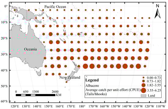
Figure 1.
Study area and distribution albacore catch per unit of effort (CPUE) from 2009 to 2019.
2.2. Data Acquisition and Processing
2.2.1. Data Source
The data for this experiment were selected from the South Pacific albacore catch data and marine environmental data from 2009 to 2019, both with a temporal resolution of months. Catch data were obtained from WCPFC (https://www.wcpfc.int/ (accessed on 7 June 2022)) and include the time of operation, location of operation (southwest corner of each 5° × 5° latitude/longitude grid cell) and catch information (number of longline hooks and tons/tails). The marine environmental data were obtained from CMEMS (https://marine.copernicus.eu/ (accessed on 20 October 2021)), including the sea surface temperature (SST), chlorophyll a concentration (Chl-a), sea surface salinity (SSS), sea surface height (SSH), ocean mixed-layer thickness (Mlotst) and sea water velocity (Vo), where the spatial resolution of Chl-a, Mlotst and Vo was 0.25° × 0.25°, while for SST, SSS and SSH, it was 0.083° × 0.083°. Tuna is sensitive to SST [36], and its survival has a higher requirement on SST, which can directly or indirectly affect the spawning and migration distribution of albacore tuna [37]; Chl-a can characterize the abundance of marine plankton. Generally, fish and shrimp feed on plankton, while albacore mainly feed on fish, squid and plankton crustaceans. Therefore, Chl-a can directly or indirectly affect the distribution of albacore [38]; SSS affects seawater buoyancy and osmotic pressure in fish, thus indirectly affecting the feeding and spawning behavior of fish, and, therefore, the distribution of fishing grounds can be distinguished using the appropriate salinity range [31]; SSH can reflect the ocean mesoscale dynamic characteristics, such as surge currents, the seawater flow rate, and hot and cold water masses, which affect the formation of fishing grounds to some extent [39]. To ensure that the environmental and spatio-temporal factors are uniformly distributed in the input layer and thus improve the forecast accuracy, the catch and marine environmental data were gridded and matched with a uniform spatial resolution of 5° × 5° in this paper. In this paper, matched 2009–2017 catch and environment data were sorted by month to construct the model training set, and the 2018–2019 data were used as the validation set.
2.2.2. Calculation of Catch Per Unit Effort (CPUE)
CPUE represents an index of resource abundance, mainly reflecting changes in the abundance of fishery resources. The calculation formula is shown in (1).
where CPUEymij denotes the CPUE within the 5° × 5° fishing ground for year y, month m, longitude i and latitude j; Catchymij and Effortymij represent the catch and fishing effort (number of hooks) within the 5° × 5° fishing ground for year y, month m, longitude i and latitude j. The units are tail/hundred hooks, tail, and hundred hooks, respectively.
2.2.3. Spatial Autocorrelation Control of Feature Variables
The mcorr function in Python 3.7 was used to plot the correlation coefficient between the target value (catch per unit effort (CPUE)) and different features of the marine environment. Based on the high correlation filter and backward feature elimination method using the SelectK-Best class of the feature_selection library, we removed features to control the correlation between CPUE and different marine environment features and the autocorrelation between marine environment features (deletion principle: ① according to the training accuracy of the model, choose a threshold (R = 0.5 in this paper) as the criterion for judging its relevance, and give priority to deleting features with low or no relevance to CPUE; ② delete the features of the marine environment with high autocorrelation between different features on the basis of the first step). As shown in Figure 2, we removed the features of the marine environment (Mlotst and Vo) that correlated with the target value (CPUE) below 0.5, and the marine environmental features (Lat, Lon, SST, SSS, SSH and Chl-a) that were ultimately used for the fishing ground classification were obtained in a sequential cycle.
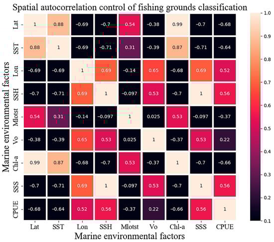
Figure 2.
Correlation of different feature variables with CPUE.
2.2.4. Normalization Process
Due to the different spatial and temporal distributions of CPUE and the large differences in the numerical ranges of environmental factors, in this paper, in order to eliminate the influence of anomalous variables and numerical range differences on the forecast results and improve the speed of model optimization and forecast accuracy, the data normalization of CPUE, SST, Chl-a, SSS, and SSH was [0–1]. The calculation formula is shown in (2).
where X′ denotes the normalized values of CPUE and environmental factors, X denotes the actual initial values, and Xmin and Xmax represent the minimum and maximum values of CPUE and environmental variables month by month, respectively.
2.2.5. Fishing Grounds Grade Classification
Tertiles provide some indication of the dispersion of the overall data distribution and are widely used in statistical studies and fishing grounds grade classification [40]. The growth habit and migration route of tuna are closely related to seasonal changes, resulting in significant differences in CPUE from month to month. Therefore, the data corresponding to the zero CPUE value were excluded from this study. The data for each month that were below the first CPUE tertiles (<33.3%) were classified as “low-yield” fishing grounds according to the tertiles, and those that were above the first CPUE tertiles (>33.3%) were classified as “high-yield” fishing grounds.
2.3. Research Method
This paper aimed to achieve high-accuracy forecasting of different grades of albacore fishing grounds in the South Pacific based on five machine learning algorithms for ensemble learning. The overall technical route is shown in Figure 3. The main contents include: (1) pre-processing based on the South Pacific albacore catch data and marine environmental data from 2009 to 2019, generating feature datasets to construct an albacore fishing ground forecasting model; (2) comparison of the accuracy of different machine learning algorithms for albacore fishing ground forecasting based on feature datasets; (3) exploring the potential of the ELM for forecasting different grades of albacore fishing grounds; (4) quantitative assessment of the effects of different environmental factors on albacore fishing ground forecasts based on RF feature importance analysis.
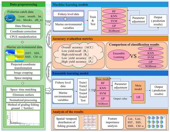
Figure 3.
Technical routes for forecasting different grades of albacore fishing grounds in the South Pacific.
2.3.1. Machine Learning Models
To compare and analyze the differences between different machine learning algorithms concerning the accuracy of albacore fishing ground forecasting, five fishing ground forecasting models, namely, KNN, SVM, XGBoost, GP and RF, were constructed in this paper based on the feature dataset of marine environmental factors. Different types of machine learning represent different classification algorithms, and each has its own advantages. The KNN algorithm has high classification accuracy and is insensitive to abnormal samples [41,42]; SVM has the advantage of being able to handle small data samples, as well as having global optimality and a strong generalization ability [43]; RF uses the average of many decision trees in the classification process to minimize overfitting and produce good regression results, thus improving the classification accuracy [44]; GP is widely used in time-series prediction tasks because of its ability to effectively exploit correlations between features [45]; XGBoost can adjust hyperparameters to maximize model performance and prevent model overfitting, while using a gradient descent optimization algorithm to integrate decision trees sequentially to minimize model error [46,47].
2.3.2. Ensemble Learning Model
This paper constructed a fishing ground forecasting model based on the South Pacific environmental factor feature dataset using the RF, SVM, KNN, XGBoost and GP algorithms for ensemble learning, which was used for the forecasting of different grades of South Pacific albacore fishing grounds. The ensemble learning model combines the outputs of different base models for forecasting, changing the single-algorithm parameterization settings by integrating the performance of individual machine learning algorithms to obtain more reliable results [7,48].
The specific process was as follows:
- The feature training dataset from 2009 to 2017 was randomly divided into training and testing sets according to the ratio of 7:3, and the training set was equally divided into train1, train2, train3, train4 and train5.
- KNN, RF, SVM, XGBoost and GP were selected as the base models for ensemble learning. For different base models, one dataset was selected as the validation set from train1 to train5 in turn, and the remaining four data were the training set for the 5-fold cross-validation to train the model accuracy. Five predictions from 70% of the training set of each base model were overlaid to generate A1–A5, and five test results from 30% of the test set of each base model were averaged to generate B1–B5.
- A1–A5 superimposed label data (Label) were used as the new training data for the logistic regression (LR) model to construct the ELM, and the classification results of different grades of fishing grounds were obtained by using five feature values (B1–B5) for classification through the ELM. The model structure is shown in Figure 4.
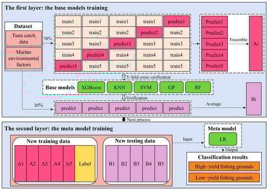 Figure 4. Flowchart of an ensemble learning fishing ground forecasting model based on the ensemble of machine learning algorithms.
2.3.3. Model Optimal Parameter Selection
To improve the forecasting ability of the model for different grades of albacore fishing grounds, this paper was based on a 10-fold cross-validation combined with the grid search method (Grid Search CV) for parameter tuning. The best values of the model parameters are obtained when the GCV reaches the minimum. The corresponding forecasting model is the best. Table 1 shows the optimal parameters of the ELM.

Table 1.
Parameter setting of each base model in the ELM.
n_estimators represents the number of decision trees of the RF model. Smaller numbers may easily cause data underfitting, while the larger the value, the better the model effect. RBF is a Gaussian kernel function in SVM, and Gamma is an essential parameter of the kernel function. max_depth indicates the maximum depth of the tree, which can effectively control the model overfitting; the larger the value, the more specific the model learning samples. CV is a hyperparameter in param_dict. C is the penalty factor; the smaller the value of C, the stronger the generalization ability of the model. leaf_size indicates the number of leaf nodes of the computed tree. n_restarts_optimizer indicates the number of times the optimizer is re-executed.
2.3.4. Model Accuracy Evaluation Metrics
In this paper, the overall accuracy (ACC), the accuracy of each type of fishing ground (P) and the recall (R) were used as indicators to evaluate the forecast accuracy of the model. The calculation formulae are shown in (3)–(5).
where ACC denotes the overall accuracy of the fishing ground forecast, Ri denotes the recall rate of class i fishing grounds, Pi denotes the accuracy of being forecasted as class i fishing grounds (the value ranges from 0 to 1; the closer to 1, the better the model forecasts, and the higher the degree of conformity between the forecasted fishing grounds and the actual fishing grounds), Ci denotes the set of the number of real fishing grounds with class i and Ci′ denotes the set of the number of fishing grounds with class i forecasted by the model (i = 1 for low-yield fishing grounds, and i = 2 for high-yield fishing grounds).
3. Results
3.1. Temporal Changes in Environment Variables
Figure 5 shows the variation in different marine environmental factors from January to December 2009–2019. In the whole time series, the value of marine environmental variable Chl-a reached its highest value in August 2012 (Chl-a = 0.172 mg/m3) and its lowest value in April 2016 (0.095 mg/m3). Furthermore, the value of Chl-a was at a low level in February–April in different years and then gradually elevated to reach higher levels in July–September, but in 2019, the highest values of Chl-a were reached in both February and July. The marine environmental variable SSS showed a decreasing, increasing and decreasing trend in the overall time series, with the highest value of SSS in October 2011 (35.51 psu) and the lowest value in March 2019 (35.04 psu). Meanwhile, the SSS reached a lower value in February–April in different years, with its peak mostly occurring in August–November of each year, but the variation in the values of SSS was lower in the months of June–August in 2012, 2016 and 2019. The marine environmental variable SST showed a decreasing and then increasing trend in the overall time series, where it reached its highest value in February 2016 (29.35 °C) and dropped to its lowest in July 2018 (24.55 °C). In different years, the value of SST was at a low level in May–August each year, while its peak occurred in January–March and September–December. The marine environmental variable SSH showed a chaotic trend in the overall time series, with no obvious change pattern, reaching its lowest value in June 2009 and 2017, with only 0.564 m in June 2017, while the peak of SSH appeared in October and December 2018, where it reached 0.726 m in December.
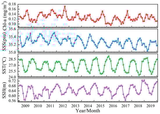
Figure 5.
Changes in different environmental factors by month from 2009 to 2019.
3.2. A comparative Analysis of the Accuracy of Machine Learning Algorithms and Ensemble Learning Model for Albacore Fishing Grounds Forecasting
To investigate the potential of ELM for forecasting different grades of albacore fishing grounds, this paper constructed ELM based on RF, SVM, KNN, GP and XGBoost algorithms for forecasting albacore fishing grounds, and the forecasting results of each model are shown in Table 2. The ELM achieved high accuracy forecasting of albacore fishing grounds (ACC = 86.92%), an overall improvement of 4.39~19.48% over the machine learning model (Table 2).
Table 2.
The average accuracy of different models in forecasting different grades of albacore fishing grounds in 2018–2019.
The average accuracy of different models for albacore fishing ground forecasting over 12 months is shown in Table 2, among which the XGBoost model obtained better fishing ground forecasting results (Figure 6). The average overall accuracy (ACC) for fishing ground forecasting over 12 months was 82.53%, the average recall for low-yield fishing grounds (R1) was 66.86%, the average precision (P1) was 77.20% and each model evaluation index was the highest. The forecast accuracy (ACC) of albacore fishing grounds was improved by 1.58~15.09% compared to other machine learning algorithms, especially for high-yield fishing grounds, where its average recall (R2) and average precision (P2) reached 90.37% and 85.01%, respectively (Table 2), proving the high accuracy of the XGBoost model for high-yield fishing ground forecasting of albacore. The RF model also achieved an average fishing ground forecast accuracy (ACC) of 80.95% for albacore over 12 months, second only to the XGBoost model, and an overall improvement of 1.58~13.51% in ACC over other machine learning algorithms. For low-yield fishing grounds, its average recall (R1) was 65.13%, and its average precision (P1) was 74.23%, while for high-yield fishing grounds, its average recall (R2) was 88.82%, and its average precision (P2) was 84.16%. The effect of the GP model on albacore fishing grounds prediction was poor (ACC = 67.44%), as shown in Figure 6, and all accuracy indicators of the model were lower than those of other algorithms. For low-yield fishing grounds, its average precision (P1) was only 51.50%, and its average recall (R1) was 58.41%, while its overall accuracy (ACC) in forecasting the fishing grounds of albacore was lower than that of other algorithms by 10.29~15.09% (Table 2). The reason for this finding may be because the GP model is less sensitive to the missing data in the dataset, the samples in the study area are unevenly distributed, the resource abundance is more scattered and there are no fishing data of albacore in some areas, leading to errors in the GP model forecasts.
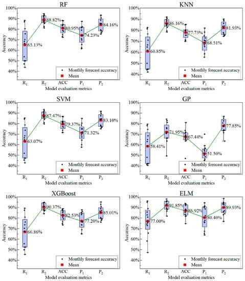
Figure 6.
Comparison and analysis of month-by-month forecast accuracy distribution and average accuracy of different models for different grades of albacore fishing grounds in 2018–2019.
Figure 6 compares the forecast accuracy of albacore fishing grounds for each month of 2018–2019 for each model, where the black points represent the forecast accuracy for each month and the red points are the mean values. The ELM returned the best forecast for albacore fishing grounds (Figure 6), and the evaluation indexes of each model were at a high level, with an average overall accuracy (ACC) of 86.92% for different months of the fishing ground forecast, along with an average recall (R2) and precision (P2) of 91.85% and 89.93% for high-yield fishing grounds, which were 1.48~19.90% and 4.92~12.08%, respectively—better than those of the machine learning algorithm overall (Table 2). The average recall and accuracy of the low-yield fishing grounds outperformed those of the machine learning model. Compared to RF, KNN, SVM, GP and XGBoost, the overall accuracy (ACC) of the ELM for the average fishing ground forecast of albacore in different months was improved by 5.97%, 9.19%, 7.55%, 19.48% and 4.39%, respectively, as shown in Table 2. The high-yield average recall R2 improved by 3.03%, 5.69%, 4.38%, 19.90% and 1.48% compared to the RF, KNN, SVM, GP and XGBoost algorithms, respectively, with the most significant improvement compared to the GP model (19.90%) and a smaller improvement compared to XGBoost (1.48%). Relative to GP, the ELM had the most significant improvement in the average precision (P1) of the low-yield albacore fishing ground forecasts (28.90%), with 12.08% for the high-yield fishing ground forecasts (P2). Relative to the XGBoost model, the ELM also improved the average recall (R1) and precision (P1) of the low-yield albacore fishing ground forecasts by 10.14% and 3.20%. This fully illustrates the stability and applicability of the ELM for forecasts of different grades of albacore fishing grounds, and the low applicability of the GP model for albacore fishing ground forecasts. The forecast accuracy indicators (R2 and P2) of the ensemble learning and machine learning models for the high-yield albacore fishing grounds were higher than those for the low-yield fishing grounds, and the forecast effect for the high-yield fishing grounds was significantly better than that for the low-yield fishing grounds (Figure 6). The reason for this finding may be that there is a difference in the rank and frequency of the first tertile of the CPUE dividing the fishing grounds, and the learner of the machine learning model will inevitably be biased towards the side with the higher frequency. In summary, among the single machine learning algorithms, the albacore fishing ground forecasting model constructed based on the XGBoost algorithm achieved better forecasts, with the RF algorithm in second place, while the GP model was less effective in forecasting the albacore fishing grounds in the South Pacific. The ELM constructed based on machine learning achieved high-accuracy forecasting of albacore fishing grounds in the South Pacific Ocean.
3.3. Ensemble Model Application Effect
To explore the application effect of the ELM on the forecast of different grades of al-bacore fishing grounds in the South Pacific, based on the longitude, latitude and environ-mental data from January to December of 2009 to 2017, the ELM was used to forecast the distribution of different grades of albacore fishing grounds from January to December of 2018 to 2019, as shown in Figure 7. Table 3 shows each accuracy index of the ELM for forecasting the distribution of albacore fishing grounds in different months. Because the operation of fishing vessels will be subject to the relevant legal system and weather con-straints in the South Pacific Ocean, CPUE does not fully represent the true grade of fishing grounds. Therefore, this paper used the high-yield recall (R2) and low-yield recall (R1) as the main evaluation indexes of the ELM for the forecast accuracy of high-yield and low-yield albacore fishing grounds in the South Pacific Ocean, respectively, and integrated other model evaluation indexes as the test method for the forecast accuracy of albacore fishing grounds.
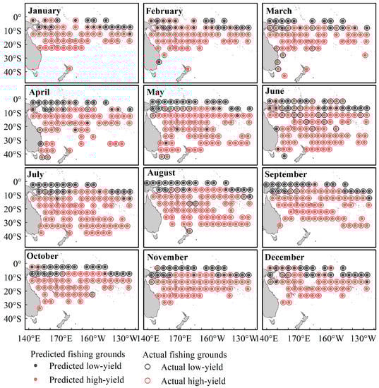
Figure 7.
Distribution of different grades of albacore fishing grounds by month in 2018–2019 based on ELM forecasts.
Table 3.
Comparison of accuracy of each evaluation index based on ELM forecasts for different grades of albacore fishing grounds in January–December 2018–2019.
To test the effect of the ELM on the forecast of different grades of albacore fishing grounds, the fishing ground grades obtained from the forecast of each month were superimposed on the real fishing ground grades in the original sea area based on the ARCGIS software (Figure 7). As shown in Table 3, the ranges of the different accuracy indicators of the ELM for the South Pacific albacore fishing ground forecast from January to December were 74.71~93.81% (ACC), 47.37~96.15% (R1), 81.82~98.00% (R2), 64.10~94.44% (P1) and 76.92~98.48% (P2). Among them, the ELM achieved the highest forecast precision (P2) for the high-yield albacore fishing grounds in January (98.48%). The high-yield fishing grounds were mainly concentrated between 10° S~25° S and 145° E~170° W, as shown in Figure 7, where the fishing grounds were more scattered in the waters between 170° W and 130° W, while no fishing grounds appeared between 25° S and 35° S. The high-yield fishing grounds appeared between 35° S~40° S and 175° E~180° waters, while the low-yield fishing grounds were mainly distributed between 0° S and 10° S, and the areas where the actual high-yield fishing grounds were incorrectly forecast as low-yield fishing grounds were almost all distributed between 0° S and 10° S. The ELM had the highest recall rate (R1 = 96.15%) for low-yield albacore fishing grounds in February (Table 3), but the high-yield recall (R2 = 81.82%) and low-yield precision (P1 = 64.10%) forecasted by the ELM for albacore fishing grounds were the lowest in February. The distribution area of the fishing grounds in February was about the same as the distribution of the fishing grounds in January, but a small number of albacore fishing grounds started to appear between 25° S and 35° S (Figure 7). In March, most of the areas where actual high-yield fishing grounds were incorrectly forecast as low-yield fishing grounds were distributed between 5° S and 10° S, and the areas where actual low-yield fishing grounds were incorrectly forecast as high-yield fishing grounds were mainly distributed between 5° S~10° S and 150° E~160° E waters.
The ELM had poor forecasting effect on low-yield albacore fishing grounds in June, among which the overall accuracy (ACC), low-yield recall rate (R1) and high-yield accuracy (P2) of the ELM were the lowest, which were 74.71%, 47.37% and 76.92%, respectively (Table 3). The fishing grounds gradually migrated southward from April to June, with the high-yield fishing grounds clustered between 10° S and 40° S and the low-yield fishing grounds showing a tendency to expand southward, which was especially obvious in June (Figure 7). The ELM was more effective in forecasting different grades of fishing grounds for high-yield albacore in September (Figure 7), where both the high-yield recall (R2) and low-yield precision (P1) were the highest at 98.00% and 94.44% (Table 3), respectively. The highest overall accuracy (ACC = 93.81%) was obtained in October for the albacore fishing ground forecast. As shown in Table 3, the forecast accuracy of the ELM for low-yield fishing grounds of albacore was not as stable as that of high-yield fishing grounds, and its recall for low-yield fishing grounds fluctuated widely in different months in terms of accuracy, while the high-yield recall was above 80% in all months. The effect of the fishing ground forecast was better, with the highest degree of conformity with the real fishing grounds (Figure 7). As can be seen in Figure 7, from July to December, the distribution of high-yield fishing grounds moved further north, with few catches south of 30° S in January–February and October–December, and most of the high-yield fishing grounds gathered in the 10° S~25° S area. In summary, most of the fishing forecast errors occurred at the junction of low-yield fishing grounds and high-yield fishing grounds. This finding may be due to the bias of the fishing grounds divided by tertiles, and the inconsistent delineation of the high-yield and low-yield boundaries in each month, making the model highly susceptible to confusion during training.
3.4. Feature Importance Analysis
The distribution of albacore fishing grounds is closely related to the geographical location of the sea area and the marine environment (SST, SSH, SSS and Chl-a). To quantitatively assess the effects of marine environmental factors on the forecast accuracy of different grades of South Pacific albacore fishing grounds, this paper explored the effects of different monthly marine environmental factors (Lat, Lon, SST, Chl-a, SSH and SSS) on the forecast accuracy of South Pacific albacore fishing grounds based on RF algorithm feature importance analysis. The RF algorithm obtains the importance ranking of each forecast factor by constructing a large number of decision trees to determine the contribution of different environmental factors to the fishing ground forecast [26,49]. The importance ranking of different marine environmental factors is shown in Figure 8.
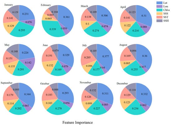
Figure 8.
Importance of different feature variables for the forecast of albacore fishing grounds by month in 2018–2019 based on ELM.
From February to December, Lat made the largest contribution to the forecast of different grades of South Pacific albacore fishing grounds, and it can be seen from Figure 8 that its contribution value was 0.224~0.377. This is because latitude is a basic factor affecting climate and is an indispensable environmental factor for the forecast of albacore fishing grounds, while the formation of environmental factors in different months is closely related to the geographical location. Chl-a had the largest effect on the forecast of albacore fishing grounds in the South Pacific Ocean in January (0.295), followed by 0.201~0.339 and 0.202~0.278 in February–May and August–December, respectively, while Chl-a had less effect on the forecast of albacore fishing grounds in other months. The importance ranking of each marine environmental factor in February was Lat > Chl-a > SSH > SST = SSS > Lon, and the importance ranking of different marine environmental factors for albacore fishing ground forecasts was the same in March, April and May (Lat > Chl-a > SST > SSH > SSS > Lon), while the contribution of each marine environmental factor to the albacore fishing ground forecasts was similar in May (Figure 8). In June–July, the influence of SST on the forecast of albacore fishing grounds exceeded that of Chl-a, with the contribution of Lat to the forecast of albacore fishing grounds reaching up to 0.377 in July, while the contribution of Lon was only 0.04. The contribution of SST was second only to Lat and Chl-a in August, September, October and December, while the importance of SSH was 0.026 higher than that of SST in November. In summary, Lat has the most significant influence on the forecast of South Pacific albacore fishing grounds and is an essential characteristic variable for the forecast of albacore fishing grounds; Chl-a and SST are important indicators of the abundance of albacore resources; and Lon makes a smaller contribution to the forecast of fishing grounds. The reason for this finding may be that albacore mainly grows in temperate waters, and temperature changes will affect the distribution of fish, while the interaction of SST and SSH may drive the intersection of hot- and cold-water masses, bringing more nutrients and attracting fish to form fishing grounds.
4. Discussion
The ELM was the most effective (ACC = 86.92%) in forecasting the South Pacific alba-core fishing grounds, with an overall improvement of 4.39~19.48% over the machine learning model. This study found that the ELM can integrate learning based on the output results of the base model as the input features of the second-layer meta-learner (LR) model, thus better integrating the advantages of the base model and producing more stable results. Meanwhile, different base models were 5-fold cross-validated, avoiding the problem of the poor generalization ability of test data division, effectively suppressing model over-fitting and improving the generalization ability and forecast accuracy of the ELM, similar to the findings of Cui et al. (2021), Q. Li and Song (2023), and Farooq et al. (2021) [20,50,51]. The XGBoost model, as a single machine learning algorithm, was better in forecasting albacore fishing grounds (ACC = 82.53%), where its overall accuracy was 1.58~15.09% better than that of other machine learning algorithms, and its accuracy (R2) in forecasting high-yield tuna fishing grounds reached 90.37%. It was found that, compared to other machine learning algorithms, the XGBoost model can effectively prevent overfitting, thus enhancing the generalization of the model and improving the accuracy of the model and the efficiency of the algorithm, similar to the findings of Lyngdoh et al. (2022) and Nguyen et al. (2021) [52,53]. The GP model was the least effective in forecasting different grades of fishing grounds, where its ACC was lower than that of other machine learning models (10.29–15.09%), and the difference in the KNN model’s forecast accuracy for low- and high-yield fishing grounds was large (R1 = 60.85%, R2 = 86.16%). This paper found that different machine learning models have certain limitations. For example, GP models are less capable of handling high-dimensional data and have high computational complexity, thus leading to performance degradation, similar to the findings of Rasmussen et al. (2005) [45]. KNN models are prone to classification bias when the category distribution is uneven, which may affect the model performance, consistent with the findings of Cover et al. (1967) [54]. In addition, the results of this study showed that the recall and precision of different algorithms in forecasting high-yield fishing grounds of albacore were better than those of low-yield fishing grounds.
The marine environment is complex and diverse, and trends in albacore activity are closely related to the marine environment [33,38,55]. It was found that, in January–February and October–December, there were few catches south of 30° S, and most of the high-yield fishing grounds were concentrated in 10° S~25° S waters, while in March and April, the distribution of fishing grounds was more scattered, but, in May–August, the albacore fishing grounds were more concentrated, and the high-yield fishing grounds were mainly distributed in 10° S~40° S waters. Additionally, this study found that most of the low-yield fishing grounds of albacore were distributed between 0° and 10° S, similar to the findings of Kühlmann (1985) [56]. Most of the high-yield fishing grounds were distributed in waters from 10° S to 40° S, showing a gradual southward expansion from January, migrating southward in early summer, and beginning to migrate northward in winter, with a clear seasonal trend in longline catches, consistent with the findings of Williams et al. (2015) [57].
It has been shown that Lat is the most important marine environmental variable for forecasting different grades of albacore fishing grounds, and it has been widely used by many scholars for forecasting fishing grounds of different marine fishes [58,59]. At the same time, marine environmental variables, such as SST, SSS, SSH and Chl-a, are also im-portant for forecasting albacore fishing grounds with high accuracy, consistent with the findings of Chen et al. (2005) and Zainuddin (2004) [31,60]. From the analysis of the im-portance of fishing ground variables (Figure 8), it can be seen that there are differences in the ranking of the importance of the contribution of marine environmental factors to the fishing ground forecasts of albacore in different months, with Lat ranking first in all months from February to December. This study found that latitude is a fundamental factor influencing climate, and that oceanic climate (SST) influences the distribution and variability of fishing grounds by affecting the growth, foraging and migration of albacore. There was also a significant effect of Chl-a on the results of the albacore fishing ground forecasts (Figure 8). It was found that changes in plankton abundance affect the abundance of fish resources as well as the distribution of fishing grounds, and that the waters around New Zealand have different trophic gradients influenced by important land as well as sub-tropical convergence zones, thus creating favorable conditions for high productivity and the development of plankton biota, similar to the findings of Vincent et al. (1991) [61]. Meanwhile, the El Niño phenomenon and wind speed in the Pacific Ocean may also affect the distribution of albacore fishing grounds. In a follow-up study, we will further explore the influence of different marine environmental factors on the forecast accuracy of albacore fishing grounds, so as to obtain more accurate fishing ground forecast information and provide technical and data support for the South Pacific fishery.
5. Conclusions
To achieve high-accuracy forecasting of albacore fishing grounds in the South Pacific Ocean, to investigate the forecasting ability of different machine learning models for alba-core fishing grounds, and to quantitatively evaluate the contribution of different marine environmental factors to fishing ground forecasting, this paper compared and analyzed the forecasting ability of the RF, KNN, SVM, XGBoost and GP machine learning algo-rithms for fishing grounds, and built an ELM based on machine learning algorithms to further improve the accuracy of fishing ground forecasting. The specific conclusions are as follows:
- The XGBoost model had a better forecast accuracy (ACC = 82.53%) for South Pacific albacore fishing grounds, which was 1.58~15.09% better than that of other machine learning models. The XGBoost and RF models have better application prospects for albacore fishing ground forecasting. The ELM was the best in forecasting albacore fishing grounds (ACC = 86.92%), and it improved the overall performance by 4.39~19.48% over the machine learning model. High-accuracy forecasting of albacore fishing grounds in the South Pacific was achieved.
- The forecast accuracy of the high-yield South Pacific albacore fishing grounds based on the ELM was more stable, with the recall of high-yield fishing grounds exceeding 80% in all months, and the forecast accuracy of the recall of low-yield fishing grounds fluctuating widely. Most of the fishing ground forecast errors occurred at the junction of low-yield fishing grounds and high-yield fishing grounds, with fewer catches in the sea near the equator. Most of the high-yield fishing grounds were distributed in the sea south of 10° S, and there was a clear seasonal trend, the grounds migrating southward in early summer and beginning to migrate northward in winter.
- Lat contributed the most to the forecast of South Pacific albacore fishing grounds in February–December, exceeding 0.224 in different months, while Chl-a had the highest importance to the forecast of albacore fishing grounds in January (0.295), and Lon had the smallest effect on the forecast of albacore fishing grounds in different months.
Author Contributions
Conceptualization, J.Z. and H.H.; methodology, J.Z.; software, D.F.; validation, B.X., Y.X. and J.S.; formal analysis, Y.X.; investigation, J.S.; resources, J.Z.; data curation, J.Z.; writing—original draft preparation, J.Z.; writing—review and editing, H.H.; visualization, D.F.; supervision, B.X.; project administration, H.H.; funding acquisition, H.H. All authors have read and agreed to the published version of the manuscript.
Funding
This research was funded by the Basic Scientific Research Ability Improvement Project for Young and Middle-aged Teachers of Universities in Guangxi (2021KY0255), the Natural Science Foundation of Guangxi Province (CN) (2022GXNSFBA035637), and the ‘Ba Gui Scholars’ program of the provincial government of Guangxi. We thank the anonymous reviewers for their comments and suggestions, which helped to improve the quality of this manuscript.
Institutional Review Board Statement
Not applicable.
Informed Consent Statement
Informed consent was obtained from all subjects involved in the study.
Data Availability Statement
Not applicable.
Acknowledgments
We thank the anonymous reviewers for their comments and suggestions, which helped to improve the quality of this manuscript.
Conflicts of Interest
The authors declare no conflict of interest, and the funders had no role in the design of the study; in the collection, analyses, or interpretation of data; in the writing of the manuscript; or in the decision to publish the results.
References
- Nikolic, N.; Morandeau, G.; Hoarau, L.; West, W.; Arrizabalaga, H.; Hoyle, S.; Nicol, S.J.; Bourjea, J.; Puech, A.; Farley, J.H.; et al. Review of Albacore Tuna, Thunnus alalunga, Biology, Fisheries and Management. Rev. Fish Biol. Fish. 2016, 27, 775–810. [Google Scholar] [CrossRef]
- Fernandez-Polanco, J.; Llorente, I. Tuna Economics and Markets. In Advances in Tuna Aquaculture; Elsevier: Amsterdam, The Netherlands, 2016; pp. 333–350. [Google Scholar]
- Lehodey, P.; Senina, I.; Nicol, S.; Hampton, J. Modelling the Impact of Climate Change on South Pacific Albacore Tuna. Deep. Deep. Sea Res. Part II Top. Stud. Oceanogr. 2015, 113, 246–259. [Google Scholar] [CrossRef]
- Pauly, D.; Belhabib, D.; Blomeyer, R.; Cheung, W.W.W.L.; Cisneros-Montemayor, A.M.; Copeland, D.; Harper, S.; Lam, V.W.Y.; Mai, Y.; Manach, F.; et al. China’s Distant-water Fisheries in the 21st Century. Fish Fish. 2013, 15, 474–488. [Google Scholar] [CrossRef]
- Mallory, T.G. China’s Distant Water Fishing Industry: Evolving Policies and Implications. Mar. Policy 2013, 38, 99–108. [Google Scholar] [CrossRef]
- Solanki, H.U.; Bhatpuria, D.; Chauhan, P. Applications of Generalized Additive Model (GAM) to Satellite-Derived Var-iables and Fishery Data for Prediction of Fishery Resources Distributions in the Arabian Sea. Geocarto Int. 2016, 32, 30–43. [Google Scholar] [CrossRef]
- Mugo, R.; Saitoh, S.-I. Ensemble Modelling of Skipjack Tuna (Katsuwonus Pelamis) Habitats in the Western North Pa-cific Using Satellite Remotely Sensed Data; a Comparative Analysis Using Machine-Learning Models. Remote Sens. 2020, 12, 2591. [Google Scholar] [CrossRef]
- Miller, T.H.; Gallidabino, M.D.; MacRae, J.I.; Owen, S.F.; Bury, N.R.; Barron, L.P. Prediction of Bioconcentration Factors in Fish and Invertebrates Using Machine Learning. Sci. Total Environ. 2019, 648, 80–89. [Google Scholar] [CrossRef]
- Rahman, L.F.; Marufuzzaman, M.; Alam, L.; Bari, M.A.; Sumaila, U.R.; Sidek, L.M. Developing an Ensembled Machine Learning Prediction Model for Marine Fish and Aquaculture Production. Sustainability 2021, 13, 9124. [Google Scholar] [CrossRef]
- Chang, Y.-J.; Sun, C.-L.; Chen, Y.; Yeh, S.-Z.; Dinardo, G. Habitat Suitability Analysis and Identification of Potential Fishing Grounds for Swordfish, Xiphias Gladius, in the South Atlantic Ocean. Int. J. Remote Sens. 2012, 33, 7523–7541. [Google Scholar] [CrossRef]
- Han, Y.; Guo, J.; Ma, Z.; Wang, J.; Zhou, R.; Zhang, Y.; Hong, Z.; Pan, H. Habitat Prediction of Northwest Pacific Saury Based on Multi-Source Heterogeneous Remote Sensing Data Fusion. Remote Sens. 2022, 14, 5061. [Google Scholar] [CrossRef]
- Harrell, F.E.; Lee, K.L.; Mark, D.B. Multivariable Prognostic Models: Issues in Developing Models, Evaluating Assumptions and Adequacy, and Measuring and Reducing Errors. Stat. Med. 1996, 15, 361–387. [Google Scholar] [CrossRef]
- Li, W.; Wu, H.; Zhu, N.; Jiang, Y.; Tan, J.; Guo, Y. Prediction of Dissolved Oxygen in a Fishery Pond Based on Gated Re-current Unit (GRU). Inf. Process. Agric. 2021, 8, 185–193. [Google Scholar] [CrossRef]
- Ömer Faruk, D. A Hybrid Neural Network and ARIMA Model for Water Quality Time Series Prediction. Eng. Appl. Artif. Intell. 2010, 23, 586–594. [Google Scholar] [CrossRef]
- Malik, W.; Boote, K.J.; Hoogenboom, G.; Cavero, J.; Dechmi, F. Adapting the CROPGRO Model to Simulate Alfalfa Growth and Yield. Agron. J. 2018, 110, 1777–1790. [Google Scholar] [CrossRef]
- Bradley, D.; Merrifield, M.; Miller, K.M.; Lomonico, S.; Wilson, J.R.; Gleason, M.G. Opportunities to Improve Fisheries Management through Innovative Technology and Advanced Data Systems. Fish Fish. 2019, 20, 564–583. [Google Scholar] [CrossRef]
- Lucas, P. Bayesian Analysis, Pattern Analysis, and Data Mining in Health Care. Curr. Opin. Crit. Care 2004, 10, 399–403. [Google Scholar] [CrossRef]
- Pan, R.; Yang, Q.; Pan, S.J. Mining Competent Case Bases for Case-Based Reasoning. Artif. Intell. 2007, 171, 1039–1068. [Google Scholar] [CrossRef]
- Cui, S.; Yin, Y.; Wang, D.; Li, Z.; Wang, Y. A Stacking-Based Ensemble Learning Method for Earthquake Casualty Prediction. Appl. Soft Comput. 2021, 101, 107038. [Google Scholar] [CrossRef]
- Zhang, Y.; Liu, J.; Shen, W. A Review of Ensemble Learning Algorithms Used in Remote Sensing Applications. Appl. Sci. 2022, 12, 8654. [Google Scholar] [CrossRef]
- Fu, B.; He, X.; Yao, H.; Liang, Y.; Deng, T.; He, H.; Fan, D.; Lan, G.; He, W. Comparison of RFE-DL and Stacking Ensemble Learning Algorithms for Classifying Mangrove Species on UAV Multispectral Images. Int. J. Appl. Earth Obs. Geoinf. 2022, 112, 102890. [Google Scholar] [CrossRef]
- Wang, Y.; Wang, D.; Ye, X.; Wang, Y.; Yin, Y.; Jin, Y. A Tree Ensemble-Based Two-Stage Model for Advanced-Stage Col-orectal Cancer Survival Prediction. Inf. Sci. 2019, 474, 106–124. [Google Scholar] [CrossRef]
- Poulos, H.; Chernoff, B.; Fuller, P.; Butman, D. Ensemble Forecasting of Potential Habitat for Three Invasive Fishes. Aquat. Invasions 2012, 7, 59–72. [Google Scholar] [CrossRef]
- Cui, S.; Wang, D.; Wang, Y.; Yu, P.-W.; Jin, Y. An Improved Support Vector Machine-Based Diabetic Readmission Pre-diction. Comput. Methods Programs Biomed. 2018, 166, 123–135. [Google Scholar] [CrossRef]
- Yao, H.; Fu, B.; Zhang, Y.; Li, S.; Xie, S.; Qin, J.; Fan, D.; Gao, E. Combination of Hyperspectral and Quad-Polarization SAR Images to Classify Marsh Vegetation Using Stacking Ensemble Learning Algorithm. Remote Sens. 2022, 14, 5478. [Google Scholar] [CrossRef]
- Dong, X.; Ju, T.; Grenouillet, G.; Laffaille, P.; Lek, S.; Liu, J. Spatial Pattern and Determinants of Global Invasion Risk of an Invasive Species, Sharpbelly Hemiculter Leucisculus (Basilesky, 1855). Sci. Total Environ. 2020, 711, 134661. [Google Scholar] [CrossRef]
- Jishad, M.; Sarangi, R.K.; Ratheesh, S.; Ali, S.M.; Sharma, R. Tracking Fishing Ground Parameters in Cloudy Region Using Ocean Colour and Satellite-Derived Surface Flow Estimates: A Study in the Bay of Bengal. J. Oper. Oceanogr. 2019, 14, 59–70. [Google Scholar] [CrossRef]
- Sydeman, W.J.; García-Reyes, M.; Szoboszlai, A.I.; Thompson, S.A.; Thayer, J.A. Forecasting Herring Biomass Using En-vironmental and Population Parameters. Fish. Res. 2018, 205, 141–148. [Google Scholar] [CrossRef]
- Mittelbach, G.G.; Ballew, N.G.; Kjelvik, M.K. Fish Behavioral Types and Their Ecological Consequences. Can. J. Fish. Aquat. Sci. 2014, 71, 927–944. [Google Scholar] [CrossRef]
- Abdul Azeez, P.; Raman, M.; Rohit, P.; Shenoy, L.; Jaiswar, A.K.; Mohammed Koya, K.; Damodaran, D. Predicting Po-tential Fishing Grounds of Ribbonfish (Trichiurus lepturus) in the North-Eastern Arabian Sea, Using Remote Sensing Data. Int. J. Remote Sens. 2020, 42, 322–342. [Google Scholar] [CrossRef]
- Chen, I.-C.; Lee, P.-F.; Tzeng, W.-N. Distribution of Albacore (Thunnus alalunga) in the Indian Ocean and Its Relation to Environmental Factors. Fish. Oceanogr. 2005, 14, 71–80. [Google Scholar] [CrossRef]
- Zainuddin, M.; Saitoh, K.; Saitoh, S.-I. Albacore (Thunnus alalunga) Fishing Ground in Relation to Oceanographic Conditions in the Western North Pacific Ocean Using Remotely Sensed Satellite Data. Fish. Oceanogr. 2008, 17, 61–73. [Google Scholar] [CrossRef]
- Pickens, B.A.; Carroll, R.; Schirripa, M.J.; Forrestal, F.; Friedland, K.D.; Taylor, J.C. A Systematic Review of Spatial Hab-itat Associations and Modeling of Marine Fish Distribution: A Guide to Predictors, Methods, and Knowledge Gaps. PLoS ONE 2021, 16, e0251818. [Google Scholar] [CrossRef]
- Daqamseh, S.; Al-Fugara, A.; Pradhan, B.; Al-Oraiqat, A.; Habib, M. MODIS Derived Sea Surface Salinity, Temperature, and Chlorophyll-a Data for Potential Fish Zone Mapping: West Red Sea Coastal Areas, Saudi Arabia. Sensors 2019, 19, 2069. [Google Scholar] [CrossRef]
- Mondal, S.; Vayghan, A.H.; Lee, M.-A.; Wang, Y.-C.; Semedi, B. Habitat Suitability Modeling for the Feeding Ground of Immature Albacore in the Southern Indian Ocean Using Satellite-Derived Sea Surface Temperature and Chlorophyll Data. Remote Sens. 2021, 13, 2669. [Google Scholar] [CrossRef]
- Lan, K.-W.; Lee, M.-A.; Lu, H.-J.; Shieh, W.-J.; Lin, W.-K.; Kao, S.-C. Ocean Variations Associated with Fishing Conditions for Yellowfin Tuna (Thunnus albacares) in the Equatorial Atlantic Ocean. ICES J. Mar. Sci. 2011, 68, 1063–1071. [Google Scholar] [CrossRef]
- Hsu, T.-Y.; Chang, Y.; Lee, M.-A.; Wu, R.-F.; Hsiao, S.-C. Predicting Skipjack Tuna Fishing Grounds in the Western and Central Pacific Ocean Based on High-Spatial-Temporal-Resolution Satellite Data. Remote Sens. 2021, 13, 861. [Google Scholar] [CrossRef]
- Sagarminaga, Y.; Arrizabalaga, H. Relationship of Northeast Atlantic Albacore Juveniles with Surface Thermal and Chlorophyll-a Fronts. Deep. Sea Res. Part II Top. Stud. Oceanogr. 2014, 107, 54–63. [Google Scholar] [CrossRef]
- Tew Kai, E.; Marsac, F. Influence of Mesoscale Eddies on Spatial Structuring of Top Predators’ Communities in the Mozambique Channel. Prog. Oceanogr. 2010, 86, 214–223. [Google Scholar] [CrossRef]
- García-Comas, C.; Chang, C.-Y.; Ye, L.; Sastri, A.R.; Lee, Y.-C.; Gong, G.-C.; Hsieh, C. Mesozooplankton Size Structure in Response to Environmental Conditions in the East China Sea: How Much Does Size Spectra Theory Fit Empirical Data of a Dynamic Coastal Area? Prog. Oceanogr. 2014, 121, 141–157. [Google Scholar] [CrossRef]
- Ren, L.; Ma, Y.; Shi, H.; Chen, X. Overview of Machine Learning Algorithms. In Lecture Notes in Electrical Engineering; Springer: Singapore, 2020; pp. 672–678. [Google Scholar]
- Boateng, E.Y.; Otoo, J.; Abaye, D.A. Basic Tenets of Classification Algorithms K-Nearest-Neighbor, Support Vector Machine, Random Forest and Neural Network: A Review. J. Data Anal. Inf. Process. 2020, 8, 341–357. [Google Scholar] [CrossRef]
- Nalluri, M.S.R.; SaiSujana, T.; Reddy, K.H.; Swaminathan, V. An Efficient Feature Selection Using Artificial Fish Swarm Optimization and Svm Classifier. In Proceedings of the IEEE 2017 International Conference on Networks & Advances in Computational Technologies (NetACT), Thiruvanthapuram, India, 20–22 July 2017. [Google Scholar]
- Wahla, S.S.; Kazmi, J.H.; Sharifi, A.; Shirazi, S.A.; Tariq, A.; Joyell Smith, H. Assessing Spatio-Temporal Mapping and Monitoring of Climatic Variability Using SPEI and RF Machine Learning Models. Geocarto Int. 2022, 37, 14963–14982. [Google Scholar] [CrossRef]
- Rasmussen, C.E.; Williams, C.K.I. Gaussian Processes for Machine Learning; The MIT Press: Cambridge, MA, USA, 2005. [Google Scholar]
- Li, Z. Extracting Spatial Effects from Machine Learning Model Using Local Interpretation Method: An Example of SHAP and XGBoost. Comput. Environ. Urban Syst. 2022, 96, 101845. [Google Scholar] [CrossRef]
- Herdter Smith, E. Using Extreme Gradient Boosting (XGBoost) to Evaluate the Importance of a Suite of Environmental Variables and to Predict Recruitment of Young-of-the-Year Spotted Seatrout in Florida; Cold Spring Harbor Laboratory: New York, NY, USA, 2019. [Google Scholar]
- Shabani, F.; Kumar, L.; Ahmadi, M. A Comparison of Absolute Performance of Different Correlative and Mechanistic Species Distribution Models in an Independent Area. Ecol. Evol. 2016, 6, 5973–5986. [Google Scholar] [CrossRef]
- Darst, B.F.; Malecki, K.C.; Engelman, C.D. Using Recursive Feature Elimination in Random Forest to Account for Cor-related Variables in High Dimensional Data. BMC Genet. 2018, 19, 65. [Google Scholar] [CrossRef]
- Pavlyshenko, B. Using Stacking Approaches for Machine Learning Models. In Proceedings of the 2018 IEEE Second International Conference on Data Stream Mining & Processing (DSMP), Lviv, Ukraine, 21–25 August 2018. [Google Scholar]
- Zhang, L.; Yang, Y.; Deng, Y.; Kang, H.; Hua-ng, T. Application of Stacking-Based Ensemble Learning Model for Water Quality Prediction. Asian Res. J. Math. 2022, 18, 69–79. [Google Scholar] [CrossRef]
- Liu, Q.; Chen, Y.; Wang, J.; Miao, H.; Wang, Y. An Example of Fishery Yield Predictions from VMS-Based Navigational Characteristics Applied to Double Trawlers in China. Fish. Res. 2023, 261, 106614. [Google Scholar] [CrossRef]
- Nguyen, H.; Vu, T.; Vo, T.P.; Thai, H.-T. Efficient Machine Learning Models for Prediction of Concrete Strengths. Constr. Build. Mater. 2021, 266, 120950. [Google Scholar] [CrossRef]
- Cover, T.; Hart, P. Nearest Neighbor Pattern Classification. IEEE Trans. Inf. Theory 1967, 13, 21–27. [Google Scholar] [CrossRef]
- Ganzedo, U.; Zorita, E.; Solari, A.P.; Chust, G.; del Pino, A.S.; Polanco, J.; Castro, J.J. What Drove Tuna Catches between 1525 and 1756 in Southern Europe? ICES J. Mar. Sci. 2009, 66, 1595–1604. [Google Scholar] [CrossRef]
- Kühlmann, D.H.H. B. B. Collette and C. E. Nauen: FAO Species Catalogue. Vol. 2, Scombrids of the World. An Anno-tated and Illustrated Catalogue of Tunas, Mackerels, Bonitos and Related Species Known to Date. = FAO Fisheries Syn-opsis No 125. Vol. 2-Mit 81 Figs., 137 Pp. Rome: FAO 1983. ISBN-Nr. 92-5-101381-0. Int. Rev. Hydrobiol. 1985, 70, 768–769. [Google Scholar] [CrossRef]
- Williams, A.J.; Allain, V.; Nicol, S.J.; Evans, K.J.; Hoyle, S.D.; Dupoux, C.; Vourey, E.; Dubosc, J. Vertical Behavior and Diet of Albacore Tuna (Thunnus alalunga) Vary with Latitude in the South Pacific Ocean. Deep. Sea Res. Part II Top. Stud. Oceanogr. 2015, 113, 154–169. [Google Scholar] [CrossRef]
- Watanabe, Y. Latitudinal Variation in the Recruitment Dynamics of Small Pelagic Fishes in the Western North Pacific. J. Sea Res. 2007, 58, 46–58. [Google Scholar] [CrossRef]
- Kokita, T. Potential Latitudinal Variation in Egg Size and Number of a Geographically Widespread Reef Fish, Revealed by Common-Environment Experiments. Mar. Biol. 2003, 143, 593–601. [Google Scholar] [CrossRef]
- Zainuddin, M.; Kiyofuji, H.; Saitoh, K.; Saitoh, S.-I. Using Multi-Sensor Satellite Remote Sensing and Catch Data to Detect Ocean Hot Spots for Albacore (Thunnus alalunga) in the Northwestern North Pacific. Deep. Sea Res. Part II Top. Stud. Oceanogr. 2006, 53, 419–431. [Google Scholar] [CrossRef]
- Vincent, W.F.; Howard-Williams, C.; Tildesley, P.; Butler, E. Distribution and Biological Properties of Oceanic Water Masses around the South Island, New Zealand. N. Z. J. Mar. Freshw. Res. 1991, 25, 21–42. [Google Scholar] [CrossRef]


Disclaimer/Publisher’s Note: The statements, opinions and data contained in all publications are solely those of the individual author(s) and contributor(s) and not of MDPI and/or the editor(s). MDPI and/or the editor(s) disclaim responsibility for any injury to people or property resulting from any ideas, methods, instructions or products referred to in the content. |
© 2023 by the authors. Licensee MDPI, Basel, Switzerland. This article is an open access article distributed under the terms and conditions of the Creative Commons Attribution (CC BY) license (https://creativecommons.org/licenses/by/4.0/).