Abstract
In recent decades, the Campi Flegrei caldera (Italy) showed unrest characterized by increases in seismicity, ground uplift, and hydrothermal activity. Currently, the seismic and hydrothermal phenomena are mostly concentrated in the Solfatara–Pisciarelli area, which presents a wide fumarolic field and mud emissions. The main fumarole in Pisciarelli is associated with a boiling mud pool. Recently, episodes of a sudden increase in hydrothermal activity and expansion of mud and gas emissions occurred in this area. During these episodes, which occurred in December 2018 and September 2020, Short Duration Events (SDEs), related to the intensity of mud pool boiling, were recorded in the fumarolic seismic tremor. We applied a Self-Organizing Map (SOM) neural network to recognize the occurrence of SDEs in the fumarolic tremor of Campi Flegrei, which provides important information on the state of activity of the hydrothermal system and about the possible phreatic activity. Our method, based on an ad hoc feature extraction procedure, effectively clustered the seismic signals containing SDEs and separated them from those representing the normal fumarolic tremor. This result is useful for improving the monitoring of the Solfatara–Pisciarelli hydrothermal area which is a high-risk zone in Campi Flegrei.
1. Introduction
Campi Flegrei is a near-circular caldera with a diameter of about 12 km (Figure 1), which includes part of the city of Naples and several smaller towns. Since 2000, Campi Flegrei caldera has been subject to long-term unrest characterized by a resumption of seismicity [1,2,3,4,5], an uplift of its central area [2,6,7,8,9,10,11,12,13], and an increase in hydrothermal activity [14,15,16,17]. In December 2012, after a phase of acceleration of geochemical changes [18], uplift, and seismicity, the Civil Protection decreed the passage to the yellow alert level (second level on a four-level scale). Since then, further gradual increases in deformation, seismic and geochemical activity have been observed, and in some cases, they have been attributed to magma intrusion [6,7,8,19,20]. The most evident variations are concentrated in the hydrothermal area of Solfatara–Pisciarelli (Figure 1), which is characterized by a powerful fumarole and a pool of bubbling mud, due to the gas flux that passes through it. In this area most of the caldera’s seismicity is concentrated, although secondary seismogenic zones are located slightly further north, and in the Gulf of Pozzuoli [2,5].
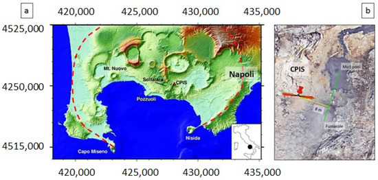
Figure 1.
(a) Map of the Campi Flegrei caldera (the coordinates are in UTM). The seismic station CPIS, in the Pisciarelli area, is marked by a red triangle, east of the Solfatara crater. The dashed red line indicates the edge of the Campi Flegrei caldera. (b) Detail of the Pisciarelli hydrothermal area showing the locations of the CPIS seismic station, 8 m from the fumarole–mud pool axis (green line).
In the hydrothermal area of Solfatara–Pisciarelli, an escalation in CO2 flux has been measured for over ten years, and is still continuing [15,16,21]. To monitor hydrothermal activity, in addition to geochemical measurements, the seismic tremor produced by the Pisciarelli fumarole–mud pool system was recorded continuously for over ten years [22]. Currently, the Pisciarelli fumarole is the most powerful emission of the Campi Flegrei caldera and one of the most powerful in Europe. The measurement and study of Pisciarelli fumarolic tremors proved to be very useful for obtaining a proxy of the CO2 flux of the fumarole–mud pool system [2,23]. Furthermore, the amplitude of the fumarolic tremor is a robust indicator of the intensity of the hydrothermal activity of the entire Solfatara–Pisciarelli area, since a good correlation between this parameter and the CO2 fluxes measured at the Bocca Grande and Bocca Nuova fumaroles of the Solfatara was highlighted in Chiodini et al. (2017) [23]. Moreover, Sabbarese et al. (2020) [24] documented a temporal evolution of the amplitude of the fumarolic tremor of Pisciarelli comparable with that of the Radon emission in the nearby Monte Olibano tunnel.
A recent study of fumarolic tremors highlighted that a sudden increase in the amplitude of this signal occurred in conjunction with the enlargement of the gas and mud emission areas in Pisciarelli on 1 December 2018 [22]. During this episode, Short Duration Events (SDEs), with a maximum duration of 0.8–1 s, were recorded in the fumarolic tremor signal, attributable to an increase in the boiling of the mud pool. The episode of 1 December 2018 raised concern for the possible evolution in phreatic activity as reported in [15]. Another episode similar to that of 1 December 2018 occurred in early September 2020, when the amplitude of the fumarolic tremor reached one of the largest values recorded so far [3].
In the present work, we analyze the two episodes of anomalous increase in fumarolic tremor amplitude that occurred in 2018 and 2020 by using an artificial neural network. Neural networks are often applied to analyze seismo-volcanic data [8,25,26,27,28,29,30,31,32,33,34,35,36,37,38,39]. Here we apply an unsupervised algorithm, the Self-Organizing Map (SOM), to cluster two main types of signal examples, namely the typical fumarolic tremor and the fumarolic tremor containing short-duration events. In particular, in this work, we developed an appropriate technique to extract the features of these two types of seismic tremors, compressing the representation of the seismic records and, at the same time, enhancing the discriminating characteristics of the two classes of signals. In the following, we first describe the data and method used in our analysis and then we present the results and discuss the implications for the monitoring of the Campi Flegrei caldera.
2. Data
We used the data recorded via the CPIS station, which is installed 8 m from the Pisciarelli fumarole and mud poll. The station is equipped with a Guralp CMG40T broadband seismometer. The sampling rate is 100 samples per second. The signal is continuously transmitted to the data acquisition center of the Osservatorio Vesuviano (Istituto Nazionale di Geofisica e Vulcanologia—INGV). Previous studies have shown that the signal generated via the fumarole–mud pool system, recorded via the CPIS station, is vertically polarized [22,23], so the measurement of the fumarolic tremor amplitude is based on the vertical component of the CPIS station. Moreover, the frequency content of this signal is generally between 5 and 15 Hz, with a peak around 8–10 Hz [22,23]. We selected two days of 2018 and eighteen days of 2020 to carry out our analysis. In particular, we chose 1 December 2018 as an example of a fumarolic tremor with SDEs (Figure 2a), and 15 November 2018 as an example of a typical fumarolic tremor signal (Figure 2b). Then, we considered the interval 25 August–11 September 2020, which contains the second episode of tremor with SDEs.
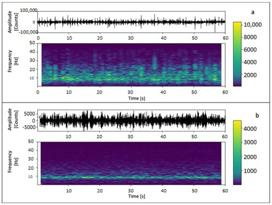
Figure 2.
Seismic signals recorded at Pisciarelli (vertical component of CPIS station) and their spectrograms. (a) The signal that was recorded on 1 December 2018 (from 23:00 UTC to 23:01 UTC), shows the presence of Short Duration Events (SDEs). (b) Typical signal of fumarolic tremor recorded on 15 November 2018 (from 00:00 UTC to 00:01 UTC).
To carry out the neural analysis, we divided the continuous signal into 1 min intervals stored in files (1440 files per day).
3. Feature Extraction
The application of the SOM network for clustering requires a data preprocessing phase. To effectively preprocess data, it is important to identify the features which characterize the seismic signals of our interest. Feature extraction allows to remove unnecessary information, reduce the size and provide a compact and robust representation of data. Choosing which features to use to describe the data is fundamental because this can affect the clustering result and therefore the performance of the neural network.
Based on the information that experts use to visually recognize seismic signals of interest, we set up a parametrization method that uses the characteristics of the waveform and the spectral content. In particular, we developed a novel ad hoc procedure to extract the features from the signals that allows us to distinguish the seismic fumarolic tremor into two main categories: that with and that without Short Duration Events.
First, we split our 20-day dataset (2 days of 2018 and 18 days of 2020) into 1 min signal windows (vertical component of CPIS station sampled at 100 Hz). Then, to remove components at frequencies outside the range of interest, we filtered each 1 min signal segment in the 2–20 Hz frequency band, which contains the signal generated via the Pisciarelli fumarole–mud pool system [22]. To parameterize the waveform of our signals, we calculated the envelope of each 1 min signal segment (Figure 3a,c). To overcome the possible effects introduced by the random cutting of the 1 min signal segment, we rearranged the obtained values in ascending order (Figure 3b,d).
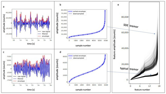
Figure 3.
Waveform parameterization. Panels (a,c) show the raw seismograms (black line), the filtered seismograms in the frequency band 2–20 Hz (blue line), and the envelope of the filtered seismograms (red line) of 6 s of tremor with SDEs recorded on 1 December 2018 and 6 s of typical fumarolic tremor recorded on 15 November 2018, respectively. Panels (b,d) show the sorted envelopes (light blue line) of a 1 min signal and the downsampling (scattered points on the dark blue line) of signals with SDEs recorded on 1 December 2018 and of typical fumarolic tremor recorded on 15 November 2018, respectively. Panel (e) shows the waveform features (18 coefficients for each 1 min signal segment) of three hours of signal, from 21:00 UTC to midnight, on 15 November and 1 December 2018.
Finally, we downsampled the sorted envelope to reduce the size of the data from 6000 to 18 parameters. The choice of the number of parameters to be used for the envelope representation is empirical and it is aimed at obtaining a good representation of the signal with the minimum number of parameters. We carried out several tests and we found that this number of parameters (18) represents a good compromise between a compact but significant data encoding.
To perform the downsampling, we adopted a variable pitch to sample more densely in the inflections of the curves obtained from the sorting of the seismogram envelopes and less densely in the quasi-linear sections (blue dots in Figure 3b,d). The effectiveness of the 18 discrete points to represent the solid line on the plots of Figure 3b,d shows the goodness of this encoding of the waveform envelope. Figure 3e shows the plot of the 18 coefficients for each 1 min signal segment of three hours of signal (180 min from 21:00 UTC to midnight) recorded on 15 November (SDE tremor) and 1 December (typical tremor), 2018. In this plot, the separation between the features obtained from the signals with SDEs and those of the typical fumarolic tremor (without SDEs) is evident for the higher values (in counts) of the tremor with SDEs and lower for the typical fumarolic tremor, and for the shapes of the curves. These observations show that this encoding allows separating the examples belonging to the two different typologies of tremor.
To obtain the spectral features we calculated the spectrum of each 1 min segment, then we smoothed it by applying a filter, and finally we downsampled the smoothed spectrum to encode the spectral content into 34 coefficients. As for the waveform envelope, also for the spectral feature representation, the choice of the number of parameters is empirical: after several tests, we found that this number allows for obtaining a good compact and significant encoding.
As in the case of the waveform feature extraction, we adopted a variable pitch in performing the downsampling to better capture the fluctuations of the smoothed spectrum. Figure 4 shows how, also in this case, the encoding in 34 discrete points is suitable for representing the smoothed spectrum of the 1 min windows of fumarolic seismic tremors. We performed the data analysis using Obspy, a Python framework for processing seismological data [40,41,42].
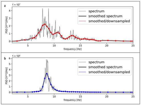
Figure 4.
Spectral feature extraction. (a) Spectrum (black line), smoothed spectrum (gray line), and downsampled smoothed spectrum (scattered points on the red line) of a 1 min signal recorded on 1 December 2018 with SDEs (00:04–00:05 UTC). (b) Spectrum (black line), smoothed spectrum (gray line), and downsampled smoothed spectrum (scattered points on the blue line) of a 1 min signal recorded on 15 November 2018 without SDEs (23:00–23:01 UTC). The symbol **2 in the title of the ordinate of both figures means "squared".
Finally, to build the feature vectors, which will be the inputs to the neural network, we combined the 34 spectral parameters with the 18 waveform ones, normalized the two series of features, and obtained our final input vectors. Figure 5 shows the input vectors (34 + 18 = 52 coefficients for each 1 min signal segment) of three hours of signal, from 21:00 UTC to midnight, on 15 November (Figure 5b) and 1 December (Figure 5a), 2018. To highlight the difference between the encoding of the two types of tremors, we also plotted the stacking of the curves (scattered points on the black lines). These input vectors will be used to perform the SOM clustering as will be shown below.
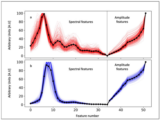
Figure 5.
The plot of the feature vectors (34 spectral parameters + 18 waveform characteristics = 52 coefficients for each 1 min signal segment) of three hours of signal (from 21:00 UTC to midnight) of fumarolic tremors extracted from 1 min signal segments recorded from 21:00 UTC to midnight recorded on 1 December 2018 with SDEs (a) and 15 November 2018 without SDEs (b). In each plot, 180 feature vectors are represented with red solid lines for tremors with SDEs (a) and with solid blue lines for tremors without SDEs (b). The stacking of the curves (black dots on the black lines) is also shown to underline the difference between the encoding of the two types of tremor.
4. Neural Analysis
4.1. SOM Method
The analysis of the extracted features was carried out using the SOM neural network [43]. The use of the SOM in this type of application is motivated by its ability to determine the intrinsic structure of the data and at the same time to test the efficiency of the proposed parameterization strategy. In future developments, we plan to create a supervised automatic system for the real-time classification of the two types of tremors using the parameterization tested with the SOM.
The SOM algorithm has been applied successfully in the field of seismology and volcanology for clustering problems [31,33,35,36,38,39,44,45,46,47,48]. Being unsupervised, it can be applied in all cases where there is no a priori information on the data as it will use similarity measures to discover their hidden structures and group them. Furthermore, as a visualization technique, the SOM realizes a non-linear projection of the data in a map that preserves their topological and metric characteristics and which, being generally two-dimensional, allows an easy interpretation of the results.
The SOM learning is competitive and cooperative: for each input presented to the network the winning node (competitive aspect) is identified, i.e., the one whose prototype is most similar to the input in terms of Euclidean distance; after that, the weights of the winning node and its topological neighbors (cooperative aspect) are updated (mathematical details in [49]). In this way, not only the winner but also its whole neighborhood is moved closer to the input pattern. The updating rule uses a decreasing neighborhood function of the distance between two nodes on the map grid, usually the Gaussian neighborhood function. The neighborhood function determines how strongly the nodes are connected to each other; this defines the region of influence that an input sample has on the SOM map. The process is iterated until the final map is obtained in which topologically near nodes contain similar inputs, generally.
The architecture of an SOM network presents two layers, one of the input neurons and one of the output neurons. Each input unit is connected to all nodes of the output layer and each of them has an associated prototype vector or weight vector, whose dimension is equal to that of the input vector. A neighborhood relation that defines the map typology or structure connects adjacent nodes.
In our application, we use a local hexagonal structure and a global toroid shape for the map, which is visualized as a sheet for simplifying the representation of clusters. Our map has a size of 4 × 3 = 12 nodes. The optimal number of nodes to use for the map cannot be established a priori because it depends on the type of application and how detailed the generated clusters must be. We have conducted several tests, varying the size of the map, and we have seen that the chosen size achieves good data clustering. The yellow hexagons identify non-empty nodes and their size corresponds to the number of input vectors that fall into each of them (data density). The gray hexagons between the yellow ones show the Euclidean distances between the nodes according to a gray scale: black or darker gray indicates a clear separation between the nodes, while white or light gray indicates similar nodes. Empty nodes are also colored using the same gray scale. In this way, it is possible to visually identify areas where the nodes are most similar to each other.
The nodes are numbered from top to bottom and from left to right as shown in Figure 6c. The choice of SOM parameters was made according to [50] and the SOM toolbox for Matlab (“http://www.cis.hut.fi/somtoolbox/ (accessed on 21 October 2022)”).
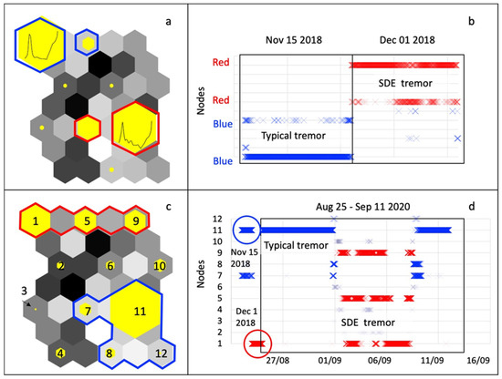
Figure 6.
(a) The SOM map with 4 × 3 = 12 nodes relative to the dataset of the two sample days, 15 November and 1 December 2018. The yellow hexagons indicate not-empty nodes and their dimension represents the data density in each node. The gray hexagons between the yellow ones show the Euclidean distance between the nodes according to a gray scale. The red cluster, formed by the two yellow hexagons outlined in red, indicates the cluster grouping the samples of tremors with SDEs. The blue cluster, formed by the two yellow hexagons outlined in blue, specifies the cluster grouping the samples of typical fumarolic tremor. For the two main nodes with the highest data density, the prototype vectors calculated via the SOM algorithm are also displayed inside them. (b) The temporal evolution of the clusters of the SOM map of panel (a) is displayed, where the input patterns of tremors with SDEs are indicated with a red x, and those of typical tremors with a blue x. (c) The SOM map with 4 × 3 = 12 nodes relative to the entire dataset of 20 days (i.e., the two sample days, 15 November and 1 December 2018, and the period 25 August–11 September 2020). The identification number is reported within the nodes of the map. Node 1 and its neighbors, i.e., nodes 5 and 6, containing tremor segments with SDEs, are marked with a red border. Node 11 and its neighbors, i.e., nodes 7, 8, and 12, containing segments of the typical fumarolic tremor, are marked with a blue border. (d) The temporal evolution of the clusters of the SOM map of panel (c) is visualized, where the input patterns of tremors with SDEs are indicated with a red x, and those of typical tremors with a blue x. The blue and red circles highlight the data for 15 November and 1 December 2018, respectively.
4.2. Results
To test our method over a short period and with temporally close data, first we applied the SOM to the dataset containing only the two sample days 15 November and 1 December 2018. This dataset consists of 2 × 1440 = 2880 1 min signal segments. Figure 6a shows the SOM clustering on this dataset. To understand which input tremor patterns, with SDEs and without SDEs, fall within each node on the map, we analyzed all the nodes of the SOM by using the labeling information associated with the name of each input file. The labeling allows classifying each file as belonging to a given temporal period. In this way, we can identify in the figure two main clusters on the map that group the signal segments of the typical fumarolic tremor (blue cluster in Figure 6a) and tremor with SDEs (red cluster in Figure 6a).
Then, we applied SOM analysis to the entire dataset (i.e., the two sample days 15 November and 1 December 2018, and the period from 25 August to 11 September 2020), which includes 20 days of data (i.e., 20 × 1440 = 28.800 1 min signal segments). Figure 6c visualizes the obtained SOM clustering. Using data labeling again, from the figure it is possible to see that the SOM map groups the tremor episodes with SDEs of 2018 and 2020 in the same cluster (red in Figure 6c) and identified a cluster of the typical fumarolic tremor (blue in Figure 6c).
Plots b and d of Figure 6 show the temporal evolution of the clusters, in the two considered datasets, highlighting the phases characterized by the occurrence of tremor with SDEs. In particular, observing Figure 6d related to the entire dataset, in the period 25 August–11 September 2020, we can note that the temporal evolution of the nodes of the SOM map indicates first the prevalence of the blue cluster until 31 August (typical fumarolic tremor), followed by the entrance of the red cluster on 1 September (tremor with SDEs), related to the anomalous phase of the beginning of September 2020, with the prevalence of node 1 on 2 and 7 September, and finally the resumption of the blue cluster on 9 September (Figure 6d), which marks the end of the anomalous activity phase.
5. Discussion and Conclusions
The Solfatara–Pisciarelli area of the Campi Flegrei caldera has recently shown episodes of a sudden increase in hydrothermal activity and mud and gas emissions. During these episodes, Short Duration Events (SDEs), related to the intensity of mud pool boiling, were recorded in the fumarolic tremor. Identifying such events can help us better define the volcano’s state of activity.
For this purpose, we have proposed a novel method to extract the features from seismic tremor data generated by the fumarole–mud pool system of Pisciarelli (central area of the Campi Flegrei caldera) and we have applied an unsupervised neural network (SOM) to cluster two different types of seismic signals, namely the fumarolic tremor with SDEs and the typical fumarolic tremor (without SDEs).
The SOM was mainly employed in this application to test how well the chosen coding for the data was able to discriminate between them. The next aim will be to use this parameterization for the creation of an automatic classification system of these two types of tremors using a supervised neural technique.
The Self-Organizing Map (SOM) is a powerful tool for data analysis exploited for several purposes. Its main advantage is that the SOM is able to cluster large, high-dimensional and complex datasets [51]. Moreover, it provides an easily understandable data representation. The reduction of dimensionality and grid clustering makes it simple to observe similarities in the data. The main drawback of SOM is that it needs necessary and sufficient data to obtain meaningful clusters. Weight vectors must be based on features that characterize the inputs well so that they can be effectively grouped and classified. A lack of data or inappropriate data in the weight vectors will degrade the performance of the method. Our feature extraction method is based on the downsampling of the sorted envelope and the downsampling of the smoothed spectrum of 1 min segments of continuous fumarolic tremor signals. This novel method for feature extraction allows a good encoding of the signals and an efficient clustering with the SOM, which effectively separates the typical fumarolic tremors from the tremors with SDEs.
The analysis of the temporal evolution of the clusters allowed us to recognize the onset of episodes of fumarolic tremors with SDEs, considered indicators of an anomalous increase in hydrothermal activity [15,22]. The occurrence of SDEs was considered linked to phases of intensification of hydrothermal activity because this type of tremor was accompanied by the expansion of the gas and mud emission areas at Pisciarelli during the episode that occurred in 2018 and could culminate in geyser-like phreatic activity. Therefore, the method we propose can improve the monitoring of the hydrothermal activity of the Campi Flegrei caldera, which is showing escalating anomalies.
Author Contributions
A.M.E., W.D.C., G.M. and F.G. conceptualization, dataset preparation, article writing, data analysis procedures, interpretation of results, article revising. All authors have read and agreed to the published version of the manuscript.
Funding
This work was supported by the Progetto ORME, INGV Project “Pianeta Dinamico”—Working Earth (CUP 1466 D53J19000170001—“Fondo finalizzato al rilancio degli investimenti delle 1467 amministrazioni centrali dello Stato e allo sviluppo del Paese”, legge 145/2018).
Institutional Review Board Statement
“Not applicable” for studies not involving humans or animals.
Data Availability Statement
The raw data supporting the conclusions of this article will be made available by the authors, without undue reservation (contact persons: Antonietta M. Esposito, email antonietta.esposito@ingv.it and Flora Giudicepietro, email flora.giudicepietro@ingv.it).
Acknowledgments
This work was partially supported by the project Progetto Strategico Dipartimentale INGV 2019. “Linking surface Observables to sub–Volcanic plumbing-system: A multidisciplinary approach for Eruption forecasting at Campi Flegrei caldera (Italy)”. G.M. and F.G. benefited from funding from the INGV Project “Ricerca Libera 2019–Study of the physical properties of the shallow structure of Vesuvius based on the analysis of seismic data.” The authors wish to thank all the many colleagues who have contributed to the monitoring effort on Campi Flegrei caldera. The authors are particularly indebted to the Istituto Nazionale di Geofisica e Vulcanologia (INGV) technical staff ensuring the regular working of the multidisciplinary monitoring networks. The data used in this study were provided by the Istituto Nazionale di Geofisica e Vulcanologia (Osservatorio Vesuviano). The authors are also grateful to the Italian Dipartimento della Protezione Civile (DPC) for supporting the monitoring activities at Campi Flegrei. This article does not necessarily represent DPC’s official opinion and policies.
Conflicts of Interest
The authors acknowledge there are no conflict of interest recorded.
References
- D’Auria, L.; Giudicepietro, F.; Aquino, I.; Borriello, G.; Del Gaudio, C.; Bascio, D.L.; Martini, M.; Ricciardi, G.P.; Ricciolino, P.; Ricco, C. Repeated fluid-transfer episodes as a mechanism for the recent dynamics of Campi Flegrei caldera (1989–2010). J. Geophys. Res. Atmos. 2011, 116, B4. [Google Scholar] [CrossRef]
- Giudicepietro, F.; Chiodini, G.; Avino, R.; Brandi, G.; Caliro, S.; De Cesare, W.; Galluzzo, D.; Esposito, A.; La Rocca, A.; Bascio, D.L.; et al. Tracking episodes of seismicity and gas transport in Campi Flegrei caldera through seismic, geophysical, and geochemical measurements. Seism. Res. Lett. 2020, 92, 965–975. [Google Scholar] [CrossRef]
- Giudicepietro, F.; Ricciolino, P.; Bianco, F.; Caliro, S.; Cubellis, E.; D’Auria, L.; De Cesare, W.; De Martino, P.; Esposito, A.M.; Galluzzo, D.; et al. Campi Flegrei, Vesuvius and Ischia Seismicity in the Context of the Neapolitan Volcanic Area. Front. Earth Sci. 2021, 9, 512. [Google Scholar] [CrossRef]
- Tramelli, A.; Godano, C.; Ricciolino, P.; Giudicepietro, F.; Caliro, S.; Orazi, M.; De Martino, P.; Chiodini, G. Statistics of seismicity to investigate the Campi Flegrei caldera unrest. Sci. Rep. 2021, 11, 7211. [Google Scholar] [CrossRef] [PubMed]
- Tramelli, A.; Giudicepietro, F.; Ricciolino, P.; Chiodini, G. The seismicity of Campi Flegrei in the contest of an evolving long term unrest. Sci. Rep. 2022, 12, 1–12. [Google Scholar]
- D’auria, L.; Pepe, S.; Castaldo, R.; Giudicepietro, F.; Macedonio, G.; Ricciolino, P.; Tizzani, P.; Casu, F.; Lanari, R.; Manzo, M.; et al. Magma injection beneath the urban area of Naples: A new mechanism for the 2012–2013 volcanic unrest at Campi Flegrei caldera. Sci. Rep. 2015, 5, 13100. [Google Scholar] [CrossRef] [PubMed]
- Trasatti, E.; Polcari, M.; Bonafede, M.; Stramondo, S. Geodetic constraints to the source mechanism of the 2011–2013 unrest at Campi Flegrei (Italy) caldera. Geophys. Res. Lett. 2015, 42, 3847–3854. [Google Scholar] [CrossRef]
- Giudicepietro, F.; Macedonio, G.; Martini, M. A Physical Model of Sill Expansion to Explain the Dynamics of Unrest at Calderas with Application to Campi Flegrei. Front. Earth Sci. 2017, 5, 54. [Google Scholar] [CrossRef]
- Iannaccone, G.; Guardato, S.; Donnarumma, G.P.; De Martino, P.; Dolce, M.; Macedonio, G.; Chierici, F.; Beranzoli, L. Measurement of seafloor deformation in the marine sector of the Campi Flegrei caldera (Italy). J. Geophys. Res. Solid Earth 2018, 123, 66–83. [Google Scholar] [CrossRef]
- Pepe, S.; De Siena, L.; Barone, A.; Castaldo, R.; D’Auria, L.; Manzo, M.; Casu, F.; Fedi, M.; Lanari, R.; Bianco, F.; et al. Volcanic structures investigation through SAR and seismic interferometric methods: The 2011–2013 Campi Flegrei unrest episode. Remote. Sens. Environ. 2019, 234, 111440. [Google Scholar] [CrossRef]
- Bevilacqua, A.; Neri, A.; De Martino, P.; Isaia, R.; Novellino, A.; Tramparulo, F.D.; Vitale, S. Radial interpolation of GPS and leveling data of ground deformation in a resurgent caldera: Application to Campi Flegrei (Italy). J. Geodesy 2020, 94, 24. [Google Scholar] [CrossRef]
- Corradino, M.; Pepe, F.; Sacchi, M.; Solaro, G.; Duarte, H.; Ferranti, L.; Zinno, I. Resurgent uplift at large calderas and relationship to caldera-forming faults and the magma reservoir: New insights from the Neapolitan Yellow Tuff caldera (Italy). J. Volcanol. Geotherm. Res. 2021, 411, 107183. [Google Scholar] [CrossRef]
- De Martino, P.; Dolce, M.; Brandi, G.; Scarpato, G.; Tammaro, U. The Ground Deformation History of the Neapolitan Volcanic Area (Campi Flegrei Caldera, Somma–Vesuvius Volcano, and Ischia Island) from 20 Years of Continuous GPS Observations (2000–2019). Remote. Sens. 2021, 13, 2725. [Google Scholar] [CrossRef]
- Chiodini, G.; Vandemeulebrouck, J.; Caliro, S.; D’Auria, L.; De Martino, P.; Mangiacapra, A.; Petrillo, Z. Evidence of thermal-driven processes triggering the 2005–2014 unrest at Campi Flegrei caldera. Earth Planet. Sci. Lett. 2015, 414, 58–67. [Google Scholar]
- Tamburello, G.; Caliro, S.; Chiodini, G.; De Martino, P.; Avino, R.; Minopoli, C.; Carandente, A.; Rouwet, D.; Aiuppa, A.; Costa, A.; et al. Escalating CO2 degassing at the Pisciarelli fumarolic system, and implications for the ongoing Campi Flegrei unrest. J. Volcanol. Geotherm. Res. 2019, 384, 151–157. [Google Scholar] [CrossRef]
- Chiodini, G.; Caliro, S.; Avino, R.; Bini, G.; Giudicepietro, F.; De Cesare, W.; Ricciolino, P.; Aiuppa, A.; Cardellini, C.; Petrillo, Z.; et al. Hydrothermal pressure-temperature control on CO2 emissions and seismicity at Campi Flegrei (Italy). J. Volcanol. Geotherm. Res. 2021, 414, 107245. [Google Scholar] [CrossRef]
- Buono, G.; Paonita, A.; Pappalardo, L.; Caliro, S.; Tramelli, A.; Chiodini, G. New insights into the recent magma dynamics under Campi Flegrei caldera (Italy) from petrological and geochemical evidence. J. Geophys. Res. Solid Earth 2022, 127, e2021JB023773. [Google Scholar] [CrossRef]
- Chiodini, G.; Caliro, S.; De Martino, P.; Avino, R.; Gherardi, F. Early signals of new volcanic unrest at Campi Flegrei caldera? Insights from geochemical data and physical simulations. Geology 2012, 40, 943–946. [Google Scholar] [CrossRef]
- Macedonio, G.; Giudicepietro, F.; D’Auria, L.; Martini, M. Sill intrusion as a source mechanism of unrest at volcanic calderas. J. Geophys. Res. Solid Earth 2014, 119, 3986–4000. [Google Scholar] [CrossRef]
- Giudicepietro, F.; Macedonio, G.; D’auria, L.; Martini, M. Insight into Vent Opening Probability in Volcanic Calderas in the Light of a Sill Intrusion Model. Pure Appl. Geophys. 2015, 173, 1703–1720. [Google Scholar] [CrossRef]
- Chiodini, G.; Caliro, S.; Cardellini, C.; Granieri, D.; Avino, R.; Baldini, A.; Donnini, M.; Minopoli, C. Long-term variations of the Campi Flegrei, Italy, volcanic system as revealed by the monitoring of hydrothermal activity. J. Geophys. Res. Atmos. 2010, 115, B3. [Google Scholar] [CrossRef]
- Giudicepietro, F.; Chiodini, G.; Caliro, S.; De Cesare, W.; Esposito, A.M.; Galluzzo, D.; Bascio, D.L.; Macedonio, G.; Orazi, M.; Ricciolino, P.; et al. Insight into Campi Flegrei Caldera Unrest through Seismic Tremor Measurements at Pisciarelli Fumarolic Field. Geochem. Geophys. Geosyst. 2019, 20, 5544–5555. [Google Scholar] [CrossRef]
- Chiodini, G.; Giudicepietro, F.; Vandemeulebrouck, J.; Aiuppa, A.; Caliro, S.; De Cesare, W.; Tamburello, G.; Avino, R.; Orazi, M.; D’auria, L. Fumarolic tremor and geochemical signals during a volcanic unrest. Geology 2017, 45, 1131–1134. [Google Scholar] [CrossRef]
- Sabbarese, C.; Ambrosino, F.; Chiodini, G.; Giudicepietro, F.; Macedonio, G.; Caliro, S.; De Cesare, W.; Bianco, F.; Pugliese, M.; Roca, V. Continuous radon monitoring during seven years of volcanic unrest at Campi Flegrei caldera (Italy). Sci. Rep. 2020, 10, 1–10. [Google Scholar]
- Dowla, F.U.; Taylor, S.R.; Anderson, R.W. Seismic discrimination with artificial neural networks: Preliminary results with regional spectral data. Bull. Seismol. Soc. Am. 1990, 80, 1346–1373. [Google Scholar]
- Röth, G.; Tarantola, A. Neural networks and inversion of seismic data. J. Geophys. Res. Atmos. 1994, 99, 6753–6768. [Google Scholar] [CrossRef]
- Romeo, G.; Mele, F.; Morelli, A. Neural networks and discrimination of seismic signals. Comput. Geosci. 1995, 21, 279–288. [Google Scholar] [CrossRef]
- Falsaperla, S.; Graziani, S.; Nunnari, G.; Spampinato, S. Automatic classification of volcanic earthquakes by using Multi-Layered neural networks. Nat. Hazards 1996, 13, 205–228. [Google Scholar] [CrossRef]
- Del Pezzo, E.; Esposito, A.; Giudicepietro, F.; Marinaro, M.; Martini, M.; Scarpetta, S. Discrimination of earthquakes and underwater explosions using neural networks. Bull. Seismol. Soc. Am. 2003, 93, 215–223. [Google Scholar] [CrossRef]
- Scarpetta, S.; Giudicepietro, F.; Ezin, E.C.; Petrosino, S.; Del Pezzo, E.; Martini, M.; Marinaro, M. Automatic Classification of Seismic Signals at Mt. Vesuvius Volcano, Italy, Using Neural Networks. Bull. Seism. Soc. Am. 2005, 95, 185–196. [Google Scholar] [CrossRef]
- Esposito, A.M.; Giudicepietro, F.; Scarpetta, S.; D’auria, L.; Marinaro, M.; Martini, M. Automatic discrimination among landslide, explosion-quake, and microtremor seismic signals at Stromboli volcano using neural networks. Bull. Seismol. Soc. Am. 2006, 96, 1230–1240. [Google Scholar] [CrossRef]
- Langer, H.; Falsaperla, S.; Powell, T.; Thompson, G. Automatic classification and a-posteriori analysis of seismic event identification at Soufrière Hills volcano, Montserrat. J. Volcanol. Geotherm. Res. 2006, 153, 1–10. [Google Scholar] [CrossRef]
- Esposito, A.M.; Giudicepietro, F.; D’Auria, L.; Scarpetta, S.; Martini, M.G.; Coltelli, M.; Marinaro, M. Unsupervised Neural Analysis of Very-Long-Period Events at Stromboli Volcano Using the Self-Organizing Maps. Bull. Seism. Soc. Am. 2008, 98, 2449–2459. [Google Scholar] [CrossRef]
- Langer, H.; Falsaperla, S.; Masotti, M.; Campanini, R.; Spampinato, S.; Messina, A. Synopsis of supervised and unsupervised pattern classification techniques applied to volcanic tremor data at Mt Etna, Italy. Geophys. J. Int. 2009, 178, 1132–1144. [Google Scholar] [CrossRef]
- Esposito, A.M.; D’auria, L.; Giudicepietro, F.; Caputo, T.; Martini, M. Neural analysis of seismic data: Applications to the monitoring of Mt. Vesuvius. Ann. Geophys. 2013, 56, S0446. [Google Scholar]
- Esposito, A.M.; D’Auria, L.; Giudicepietro, F.; Martini, M. Waveform Variation of the Explosion-Quakes as a Function of the Eruptive Activity at Stromboli Volcano. In Neural Nets and Surroundings; Springer: Berlin/Heidelberg, Germany, 2013; pp. 111–119. [Google Scholar]
- Zhu, W.; Mousavi, S.M.; Beroza, G.C. Seismic Signal Denoising and Decomposition Using Deep Neural Networks. IEEE Trans. Geosci. Remote. Sens. 2019, 57, 9476–9488. [Google Scholar] [CrossRef]
- Giudicepietro, F.; Esposito, A.M.; Spina, L.; Cannata, A.; Morgavi, D.; Layer, L.; Macedonio, G. Clustering of Experimental Seismo-Acoustic Events Using Self-Organizing Map (SOM). Front. Earth Sci. 2021, 723, 581742. [Google Scholar] [CrossRef]
- Giudicepietro, F.; Calvari, S.; D’Auria, L.; Di Traglia, F.; Layer, L.; Macedonio, G.; Caputo, T.; De Cesare, W.; Ganci, G.; Martini, M.; et al. Variations of Stromboli activity related to the 2019 paroxysmal phase revealed by SOM clustering of seismo-acoustic data and its comparison with video recordings and GBInSAR measurements (No. EGU22-10482). In Proceedings of the EGU General Assembly 2022, Vienna, Austria, 23–27 May 2022. [Google Scholar]
- Beyreuther, M.; Barsch, R.; Krischer, L.; Megies, T.; Behr, Y.; Wassermann, J. ObsPy: A Python Toolbox for Seismology. Seism. Res. Lett. 2010, 81, 530–533. [Google Scholar] [CrossRef]
- Megies, T.; Beyreuther, M.; Barsch, R.; Krischer, L.; Wassermann, J. ObsPy–What can it do for data centers and observatories? Ann. Geophys. 2011, 54, 47–58. [Google Scholar]
- Krischer, L.; Megies, T.; Barsch, R.; Beyreuther, M.; Lecocq, T.; Caudron, C.; Wassermann, J. ObsPy: A bridge for seismology into the scientific Python ecosystem. Comput. Sci. Discov. 2015, 8, 014003. [Google Scholar] [CrossRef]
- Kohonen, T. Self-organized formation of topologically correct feature maps. Biol. Cybern. 1982, 43, 59–69. [Google Scholar] [CrossRef]
- D’Auria, L.; Esposito, A.M.; Petrillo, Z.; Siniscalchi, A. Denoising Magnetotelluric Recordings Using Self-Organizing Maps. In Advances in Neural Networks: Computational and Theoretical Issues; Springer: Cham, Switzerland, 2015; pp. 137–147. [Google Scholar]
- Carbonari, R.; Di Maio, R.; Piegari, E.; D’Auria, L.; Esposito, A.; Petrillo, Z. Filtering of noisy magnetotelluric signals by SOM neural networks. Phys. Earth Planet. Inter. 2018, 285, 12–22. [Google Scholar] [CrossRef]
- Esposito, A.M.; Giudicepietro, F.; Scarpetta, S.; Khilnani, S. A Neural Approach for Hybrid Events Discrimination at Stromboli Volcano. In Multidisciplinary Approaches to Neural Computing; Springer: Cham, Switzerland, 2018; pp. 11–21. [Google Scholar]
- Esposito, A.M.; De Bernardo, A.; Ferrara, S.; Giudicepietro, F.; Pappalardo, L. SOM-Based Analysis of Volcanic Rocks: An Application to Somma-Vesuvius and Campi Flegrei Volcanoes (Italy). In Neural Approaches to Dynamics of Signal Exchanges; Springer: Singapore, 2020; pp. 55–60. [Google Scholar]
- Esposito, A.M.; Alaia, G.; Giudicepietro, F.; Pappalardo, L.; D’Antonio, M. Unsupervised Geochemical Analysis of the Eruptive Products of Ischia, Vesuvius and Campi Flegrei. In Progresses in Artificial Intelligence and Neural Systems; Smart Innovation, Systems and Technologies; Springer: Singapore, 2021; Volume 184. [Google Scholar] [CrossRef]
- Kohonen, T. Self-Organizing Maps, Series in Information Sciences 30, 2nd ed.; Springer: Berlin/Heidelberg, Germany, 1997. [Google Scholar]
- Kohonen, T.; Hynninen, J.; Kangas, J.; Laaksonen, J. SOM_PAK: The self-Organizing Map Program Package, Report A31, Helsinki University of Technology, Laboratory of Computer and Information Science, Espoo, Finland. 1996. Available online: www.cis.hut.fi/research/som_lvq_pak.shtml (accessed on 21 October 2022).
- Pang, K. Self-organizing maps. J. Neural Netw. 2003. Available online: https://www.cs.hmc.edu/~kpang/nn/som.html (accessed on 25 April 2023).


Disclaimer/Publisher’s Note: The statements, opinions and data contained in all publications are solely those of the individual author(s) and contributor(s) and not of MDPI and/or the editor(s). MDPI and/or the editor(s) disclaim responsibility for any injury to people or property resulting from any ideas, methods, instructions or products referred to in the content. |
© 2023 by the authors. Licensee MDPI, Basel, Switzerland. This article is an open access article distributed under the terms and conditions of the Creative Commons Attribution (CC BY) license (https://creativecommons.org/licenses/by/4.0/).