1. Introduction
Autonomous driving has become a broad research topic in recent years, and it has great potential to enhance driving safety and improve transport efficiency [
1]. An autonomous driving system includes many modules, such as decision, planning, and control modules [
2], which require accurate knowledge of the vehicle’s position to perform correct driving decisions and actions [
3]. For example, an error of a few decimeters may cause the vehicle to position itself in the wrong lane, leading to incorrect driving decisions, and thus to traffic accidents. Therefore, self-driving cars require robust localization systems with decimeter-level or even centimeter-level accuracy [
4].
Global navigation satellite systems (GNSS) [
5] are the most commonly used method for vehicle localization. A GNSS is suitable for open areas but is less reliable in obscured environments involving structures such as tall buildings and viaducts due to signal occlusion, multipath errors, and other factors. A GNSS can reach the centimeter level in open areas with real-time kinematic (RTK) [
6] technology; however, the effect of multipath errors on localization estimates persists, so GNSS alone cannot provide consistent and reliable localization accuracy. A GNSS is usually integrated with an IMU [
7] to form a localization system. IMUs consist of accelerometers and gyroscopes, which can measure vehicle acceleration and angular velocity. This information can be further used to calculate vehicle position relative to its initial position in a process called dead reckoning. However, IMU measurements are affected by multiple noises that are amplified during the multiple integrations of acceleration to displacement and angular velocity to attitude angle, grow exponentially, and accumulate over time.
Wheel odometry measures the number of pulses per unit of time at the wheel through wheel encoders to calculate wheel speed and travel distance. Due to the necessity of an anti-lock brake system (ABS), wheel encoder sensors are mounted on the vehicle, making wheel odometry a localization technology that can be used universally. Compared to IMU’s accelerometer sensors, wheel odometry requires fewer integration steps to determine the vehicle position, reducing errors in the integration process and providing a better positioning solution. Wheel odometry was initially widely used in mobile robotics and was then gradually applied to vehicles to complete localization tasks. Thrun, S et al. [
8] improved the problem of poor estimation of vehicle attitude and IMU bias when GNSS signals are weak or down, which occurs in common GNSS/IMU fusion algorithms, by considering wheel odometry. Funk, N et al. [
9] complemented visual–inertial odometry with wheel odometry for automotive applications. In addition, wheel odometry can be the primary localization algorithm in some special cases, such as low light conditions, low speed driving, and parking scenes [
10,
11].
The accuracy of wheel odometry-based localization is affected by many factors; on the one hand, it is affected by model parameters, such as tire diameter. Although these can be calibrated during installation, they can change dynamically when the vehicle is driven due to certain factors, such as wheel wear and load changes, which can affect the odometry output. On the other hand, the measurement accuracy of odometry is affected by wheel slip. In addition, unevenness on the road surface, such as bumps and potholes, interferes with the odometry results. Therefore, the output errors of wheel odometry have high uncertainty, and accurately predicting the wheel odometry error is key to improving wheel odometry-based localization accuracy.
Fazekas, M et al. proposed an off-line iterative estimation algorithm in [
12] and an online estimation method in [
13] in which Kalman filter and the least squares algorithm are performed in an iterative loop for wheel circumference estimation of autonomous vehicles to improve wheel odometry’s accuracy. They further estimated the wheel circumferences recursively to improve the wheel speed estimation with a nonlinear least squares method in [
14]. The study [
15] calibrated the parameters of the wheel odometry model with Gauss–Newton regression and Kalman filter. Welte A et al. [
16] presented a method able to accurately calibrate the model parameters by using a Rauch–Tung–Striebel smoothing scheme which enables to obtain state estimates close to the ground truth. In summary, these studies used traditional state estimation methods to improve wheel odometry’s accuracy. However, these methods rely on precise parameter adjustment, which lacks adaptability to various driving conditions. On the other hand, the wheels are affected by many factors of road conditions and their own parameters so that it is difficult to obtain an accurate model under the action of multiple factors using traditional state estimation methods. Deep learning is a data-driven approach that can learn complex nonlinear properties and uncertainty from data. Researchers have proposed deep learning-based techniques to discover the error drift characteristics of IMUs over time for better GPS/INS combined navigation solutions [
17,
18,
19,
20]. Several deep learning techniques have also been applied to wheel odometry: an LSTM model was proposed to learn the uncertainty of wheel odometry in [
21], and a WhONet model was proposed in [
22], which further improved the performance compared to the LSTM model.
The transformer model [
23] emerged in the field of natural language processing (NLP), and it was first used for machine translation tasks to achieve SOTA effects. A transformer model can fully utilize the GPU resources for parallel computation to accelerate the training speed. Compared with traditional models such as RNN and LSTM that deal with time series, transformer models do not rely on past hidden states to capture the dependence on previous information but learns the association of information at each moment in a time series as a whole, avoiding the risk of losing past information and reducing the performance degradation caused by long-term dependence.
This study aims to explore a new low-cost localization method that combines wheel odometry and deep learning techniques. The main contributions of this paper are as follows:
A transformer-based error prediction model is developed to learn the measurement uncertainty of wheel odometry, and the end-to-end correspondence from the wheel speed to the travel distance error is established. Tests on a publicly available dataset and an experimental vehicle are performed to verify that the proposed model can accurately predict the output error of wheel odometry and improve the accuracy, stability, and reliability compared to LSTM and WhONet under various driving conditions. In addition, the model trained using the public dataset is transferred to the experimental vehicle to verify the model’s generalization capability and the improved positioning performance of dead reckoning by combining the model.
Driving condition characteristics, including features describing road types, road conditions, and vehicle driving operations, are considered. Models with different inputs are developed and compared, one with and the other without driving condition characteristics. The tests demonstrate that the model that considers driving characteristics has better adaptability to longer GNSS outage driving conditions.
The rest of the paper is organized as follows:
Section 2 describes the dead reckoning method based on wheel odometry;
Section 3 presents the Transformer model and the selected input features;
Section 4 defines the dataset and metrics used to train the model and evaluate its performance, as well as the model parameters, in addition to showing the process of model parameter tuning;
Section 5 demonstrates the results based on a publicly available dataset and when the model is applied to real vehicles, followed by a relevant discussion; finally, the entire paper is concluded in
Section 6.
2. Dead Reckoning Based on Wheel Odometry
The dead reckoning (DR) system relies on odometry, which measures the distance traveled by the vehicle, and the angular velocity obtained from the chassis or a gyroscope in IMUs, to estimate the relative position forward from the current position.
The wheel odometry is based on wheel encoders to track the number of revolutions each wheel has made, and each wheel’s measured angular velocity can be derived. Then, the distance traveled by each wheel per unit of time is calculated by combining the wheel radius. According to wheel odometry, the vehicle’s measured travel distance from moment
to moment
can be expressed as:
where
and
are the measured left and right rear wheel angular velocities, respectively, and
r is the nominal wheel radius.
Many factors influence the measurement accuracy of wheel odometry. First, the measurement of wheel angular velocity contains errors; second, some factors, such as the vehicle load changes, change the wheel radius dynamic; third, some aspects, such as wheel slip and road potholes, lead to the wheel rolling distance not being equal to the actual distance the vehicle travels.
The vehicle’s real travel distance from moment
to moment
can be expressed as:
where
is the error of the actual left rear wheel angular velocity compared with
,
is the error of the real right rear wheel angular velocity compared with
,
is the error between
r and the real left rear wheel radius during vehicle driving,
is the error between
r and the real right rear wheel radius during vehicle driving, and
is the error between the rolling distance and the actual travel distance.
Let
be the error of the travel distance:
where
is the measured travel distance.
In practice, the point coordinates measured by RTK-GPS have centimeter-level accuracy and can be regarded as the true value of the localization coordinates. Suppose
are the recorded points from moment
to moment
, then
can be expressed as:
where
is the distance between
and
on the Earth’s surface, which can be calculated according to the Vincenty formula given in [
24].
Suppose the vehicle’s travel distance in a short time
is
and the vehicle’s heading angle is
, the transverse and longitudinal displacements
and
are:
The relative displacements between two moments
and
can be regarded as accumulating relative displacements in a very short time
. Therefore, the transverse displacement
and the longitudinal displacement
from moment
to moment
can be expressed as:
According to Equations (5)–(8), after obtaining the travel distance between adjacent moments with the wheel odometry, the vehicle’s relative displacement between two moments can be calculated by combining the vehicle’s heading angle.
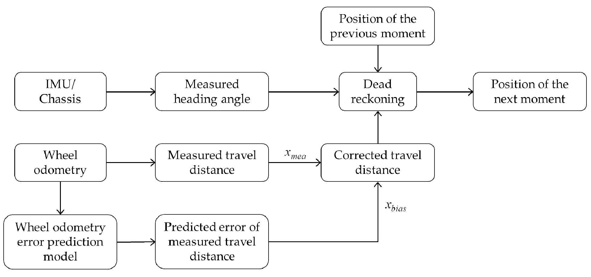
Figure 1 shows the role of the wheel odometry error prediction model in the localization system. With the established model, the travel distance error can be predicted accurately, and the travel distance output by the odometry can be corrected so that a more accurate position of the next moment can be obtained after dead reckoning.
3. Transformer Model
As the output of wheel odometry is affected by many factors, the measurement error has high uncertainty and keeps changing and accumulating over time. Transformer is a deep learning model that processes time series, and the use of Transformer is studied in this paper to learn the error characteristics of wheel odometry from time series for more accurate localization. In this section, a Transformer-based error prediction model is established to predict the error of the wheel odometry output.
The Transformer model is based on encoder/decoder architecture. The original input is translated into the model input containing location information through embedding and location coding. The encoder consists of a stack of N identical layers with two sub-layers. The first sub-layer is a multi-head self-attention layer used to extract the features of different attention heads of the model. The second sub-layer is a fully connected feed-forward network, which can enhance the nonlinear representation ability of the model. Both sub-layers use residual connection and normalization. Residual connection further enhances the fitting ability of the model, and normalization can avoid the problem of the slow convergence of the model caused by the parameters being too large or too small. The decoder is also composed of N identical layers stacked. In addition to the two sub-layers in each encoder layer, the decoder inserts a third sub-layer, which is used to perform a multi-head attention calculation on the output of the last encoder. Similar to the encoder, the decoder uses residual connection and normalization for each sub-layer. The first self-attention sub-layer of the decoder is designed in a masked form to ensure that the prediction of position i depends only on the known output at positions less than i. The output of the decoder is converted to the required dimension through a linear layer, and the value with the highest probability calculated through the softmax layer is the final output of the model.
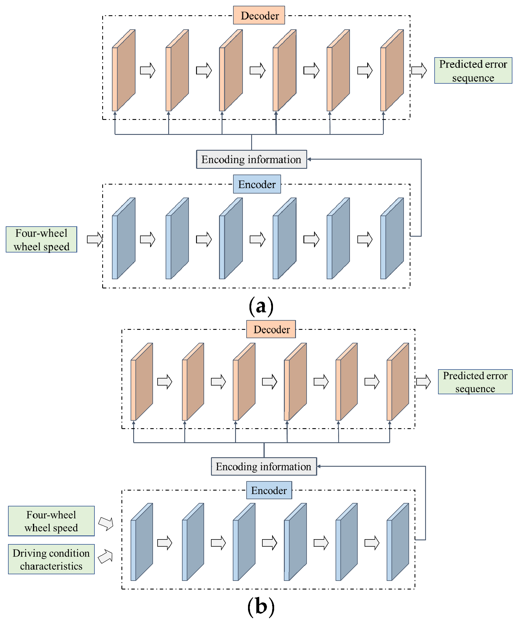
Considering that different driving conditions may influence the wheel states and affect the odometry output, two different Transformer error prediction models are designed. The first model contains four-wheel wheel speed as the input to the encoder, and the second model considers the driving condition features and four-wheel wheel speed as the input to the encoder. Both models output the predicted error sequence. The Transformer model that does not consider the driving conditions is referred to as Transformer-NDC for convenience, and the Transformer model that considers the driving conditions is referred to as Transformer-DC for convenience. The structures of the two models are shown in
Figure 2.
Referring to the different driving conditions in the public dataset (IO-VNBD) [
25] and common driving condition features, a total of 29 features describing different driving conditions were selected, as shown in
Table 1. Features 1–9 describe different road types, features 10–15 describe different road conditions, and features 16–29 describe various vehicle driving operations. The data subsets are preprocessed in combination with the selected features. The feature value takes the value of 1 when the corresponding driving condition of the data subset contains the related feature; otherwise, it takes the value of 0.


