1. Introduction
The car-following (CF) model was established to describe how a driver reacts to the leading vehicle in the longitudinal direction, which is the most basic driving behavior [
1]. The precision with which CF models can replicate the behavior is of paramount importance for traffic operation and safety, for example, precise CF modeling can benefit our understanding of the mechanisms of traffic congestion evolution and the study of negative externalities in traffic flow such as oscillations [
2]. It also can provide reliable behavioral support for adaptive cruise control strategies in advanced driving assistance systems (ADASs) [
3]. Thus, in past decades, many efforts have been made to narrow the gap between the CF model outputs and the actual human driving behavior through model comparisons or improvements in structure. Essentially, most of these models are formulated so that the simulated driver follows a long-term intrinsic law defined by initial unified parameters, referred to as driver-based modeling (DBM) in this study.
However, affected by the dynamic human–vehicle–road environment system, drivers will correspondingly change the CF process’s behavior [
4,
5]. This intra-driver variance can be recognized as the occasional short-time and common behavior variance in different driving modes [
6]. The former is an occasional behavior in the CF process, and the location of these events in the record is relatively clear, usually caused by obvious abnormal changes in the external environment. On the contrary, the driving mode, defined as a certain behavior consistency or repetition in the CF interaction in a time segment, can be viewed as the basic component of CF behavior. Both objective environmental changes and subjective adjustments of drivers in driving task realization can lead to behavior variance in different driving modes, which almost exists in all the CF events. However, the core pathway of the current DBM is to apply a complex mapping function to pool what are essentially different states and, as a result, the CF model based on the DBM is likely to be inaccurate in the description of each mode, but to achieve a kind of average we lower the total error level. Therefore, the concept of driving-mode-based modeling (DMBM) is proposed; that is, to convert the parameters of a CF model from the mapping of different drivers to the mapping of different driving modes. However, our understanding of driving modes remains limited. Specifically, there is a dearth of knowledge regarding the fundamental modes that constitute the car-following process and how the behavior of these different driving modes influences the accuracy of existing car-following models.
To recognize several basic CF behavior modes from massive empirical driving data is a process of segmenting data and then categorizing these segments according to the potential data characteristics. A long multivariate CF time series is to be segmented into short sequences which contain repeatedly reoccurring behavior “patterns” or “modes”, such as certain slight fluctuations in the velocity dimension. For consistency, we use “mode” to refer to it. Meanwhile, these short sequences of common repeat features will be labeled with the same mode number. Conventionally, the rule-based division is applied. Taking a common example, the classical Wiedemann model consists of different threshold-determined state–action regimes representing drivers’ differentiated behavior modes, such as unconscious reaction, reaction, deceleration, etc. Nevertheless, this mode segmentation is subjective and provides less insight into structural similarities in the data, and therefore the Wiedemann model has not shown advantages in modeling accuracy in the past compared with those traditional nonlinear models based on the DBM [
1]. In contrast, an unsupervised data-driven method is more promising and adaptable for this question. Recently, Higgs et al. [
7] applied a distance-based time series clustering method to the CF records and found up to 30 driving modes for car drivers and another 30 modes for truck drivers. This quantity is outside of the scope of the basic driving modes we are aiming to investigate, which will lead to an unacceptable number of parameters if it is applied to the DMBM. Furthermore, conventional clustering methods relying on distance-based metrics may emphasize matching values rather than searching for nuanced structural similarities in the CF process. In summary, how to precisely segment and determine CF behavior modes from empirical data records remains elusive.
Furthermore, both the volume and accuracy of data are critical for accurately identifying potential subtle data changes and dependencies in different driving modes through data-driven approaches. Despite the increasing use of real-world trajectories in CF model calibration and comparison [
8,
9], due to the development of data collection and storage, the accuracy of some commonly used data cannot be well guaranteed. For example, Next Generation Simulation (NGSIM) data [
10], a contributive dataset has been widely adopted in traffic flow and travel behavior modeling, has also been criticized for its accuracy issues [
11]. On the other hand, for comparison with the DBM, sufficient records for each driver are necessary to obtain accurate fitting parameters for drivers. Some recent datasets such as High D [
12] have indeed been improved with new recording approaches, but their observations of each driver are extremely limited. Higgs et al. introduced naturalistic driving data with long records for each driver, but the fact that there are only ten drivers for each type of vehicle limits the credibility of the results.
Therefore, to fully overcome the challenges mentioned above, we first introduce a novel data-driven approach, named Toeplitz Inverse Covariance-based Clustering (TICC), to solve the driving modes mining. Then, a large-scale naturalistic driving study (NDS) is adopted to validate and compare the DMBM and the DBM. The main contributions of this study are:
With up to 40 representative drivers from the large-scale NDS data, a total of 4000 high-resolution CF events were extracted for CF behavior modes mining. The duration of each event is longer than 30 s to guarantee that more continuous data dependencies in the CF behavior can be found;
An accurate subsequence clustering tool of multivariate time series, TICC, is introduced for driving mode recognition. Rather than conventional distance-based clustering, it is based on the graphical dependency structure of each subsequence to recognize the potential reoccurred CF behavior patterns more precisely;
The number of CF behavior modes is determined by careful consideration of the clustering results and the CF behavior modeling results. Based on this, a comparison of the DBM and the DMBM is conducted to demonstrate the potential of the DMBM to improve the accuracy of CF modeling.
The rest of this paper is organized as follows.
Section 2 reviews the related works regarding CF behavior and mode discovery techniques;
Section 3 describes the data information and extraction of CF events;
Section 4 details the methodology of mode recognition and CF model calibration;
Section 5 determines the number of driving modes and shows the modeling performance;
Section 6 provides discussions; and
Section 7 concludes the study and discusses future work.
2. Related Works
In the past several decades, a multitude of car-following models have been developed and refined to more accurately replicate human car-following behavior. These models are optimized using specific sets of parameters that best fit the driving characteristics of individual drivers. In a conventional way, most CF models are the mapping functions of different drivers’ full trajectories, but some researchers have noticed that there are different driving behavior modes or patterns in the CF process, which can be viewed as correlations of behavioral characteristics. In this section, we summarize related works from the following three perspectives: (1) CF behavior modeling, (2) driving modes in CF, and (3) mode discovery of time series.
2.1. CF Behavior Modeling
In the past seventy years, consideration of developing and improving CF behavior modeling, which is one of the foremost fundamental driving behaviors, has been ongoing. Various mapping functions, ranging from simple linear equations to complex sets of nonlinear equations, have been proposed to better understand interactions between following vehicles and leading vehicles in non-free traffic flow. Four fundamental models have been proposed and well-developed and have been demonstrated to be reliable in simulation practices: stimulus-response logic, safety distance logic, desired measures logic, and perceptual-thresholds logic. While attempts based on machine learning techniques have been made, they are beyond the scope of this paper due to limitations in the analysis of human-driven mechanisms, which hinders further applications.
First, the stimulus-response CF model is commonly recognized as the foremost classical CF interaction logic. This kind of model takes the interaction characteristics between the CF pair as a “stimulus”, based on which the following vehicle makes “responses” accordingly. Commonly adopted factors that are considered as stimuli include the velocity of the leading vehicle, spacing between the CF pair, and the velocity difference [
13]. Numerous upgraded and advanced forms of the original version proposed by Chandler et al. [
14] have been proposed, such as models with memory [
15], or acceleration and deceleration asymmetry [
16]. Second, Kometani [
17] initially defined the safety distance logic. The main hypothesis of this logic is that gaps between the CF pair are more linked to driver response rather than relative velocities. Nonlinear constructs were introduced to fulfil this logic by Newell [
18]. There is also a model proposed by Gipps [
19] that increased the adaptability with several human behavioral parameters considered, such as reaction time and desired velocity, which has been the most popular in its category. Third, models based on the concept of the desired measures were established by Helly [
20]. Differing from the logics above, drivers are supposed to achieve expected values of CF characteristics such as time headway. Another famous and well-adopted model is the intelligent driver model (IDM). The IDM is proven to be most accurate and adaptable in reproducing the CF behaviors of drivers, and it remains accurate when applied to different driving styles or different traffic flow facilities [
1].
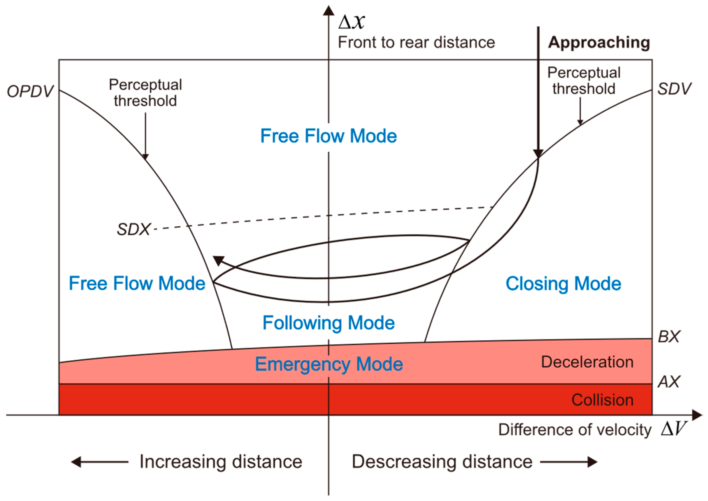
Finally, to avoid neglecting the impact of human psychological reactions, a new concept based on “perceptual threshold” was proposed by Wiedemann. It is supposed that not all stimuli from CF pair interactions can lead to subjective operations from the following vehicle. The threshold of perception for a driver is defined as the minimum value of a stimulus that can be detected and elicit a response. Therefore, a dynamic threshold is used to distinguish between free-flow mode or CF mode, which is one of the innovations of this model [
13]. In essence, it is one of the few models that can reproduce the following behavior from different driving phases or modes and divide and conquer for each mode. Then, researchers attempted to improve the accuracy of the Wiedemann model by changing the sub-model with the GHR model [
21]. However, the driving modes division in these models is relatively subjective and lacks empirical verification. The thresholds that divide different CF modes, such as SDV, BX, SDX, etc. [
22], were subjectively proposed based on the theoretical hypothesis, and it is difficult to find empirical evidence to prove that these modes are consistent with realistic driving modes in human CF behavior. Additionally, the Wiedemann model shows disadvantages in the comparison of CF models over the IDM with much more behavioral parameters [
1], while the latter only contains free-flow mode and CF mode.
Despite the approach of perceptual-thresholds logic, the aforementioned models are based on the assumption of a single mapping function for each driver. Consequently, regardless of the complexity of the mapping function, these existing methods may still produce errors due to pooling essentially different modes. Moreover, there is still an insufficient and fragmented understanding of driving modes in the car-following process.
2.2. Driving Modes in the CF Process
The formulation of human behavior is a highly complex process influenced by a multitude of factors, including individual physiological and psychological characteristics, interpersonal interactions, and external environmental conditions [
1]. To address the oversimplifications inherent in modeling such a complex process, numerous studies have endeavored to elucidate the variability in CF behavior. Most of them focused on occasional unusual behavior, such as distraction or short-time variance caused by cut-ins, but less attention was paid to the CF process’s basic modes.
A simple attempt is to divide the CF process according to the acceleration. Drivers in the accelerating and decelerating process will adopt different driving strategies [
23], which is named asymmetric driving behavior and needs to be modeled separately [
24], but there is less insight into the division of driving modes since only two modes can be provided and investigated. Meanwhile, Higgs et al. [
7] viewed the driving process as the mapping function of a driver’s reaction and the driving state variables, in which driving modes are the different divided parts of the state space. They adopted a two-step algorithm and clustered up to 30 driving modes from 10 car drivers, but the quantity is out of the scope of the fundamental driving modes; therefore, it is almost impossible to be applied in the simulation practices due to the considerable number of parameters. Some researchers, such as Lin et al. [
25], attempted to discover the modes of sub-state transition in CF to divide driving modes, but, essentially, there still exists different behavior relevance in each mode.
As viewed above, although attempts have been made to decompose CF behavior and find some basic modes, the results are not satisfactory and still cannot answer what repetitive correlations of behavioral characteristics make up the CF behavior.
2.3. Mode Discovery of Time Series
Multivariate time series are exceptionally common, existing in various areas such as engineering, science, or finance, which often contain some repeatedly occurring modes. The differences between those modes can be very small. Discovering those modes contributes to realizing the underlying mechanisms, while in this study, we are attempting to apply a proper tool to find the behavioral modes which exist in the CF process.
A lot of work has been done to cluster similar modes from time series, but fewer are introduced to discover the modes in the CF or even in transportation engineering [
7]. In terms of data dimensionality, the research can be broadly categorized into two primary groups: univariate and multivariate clustering. In this study, we mainly focused on the latter. In multivariate clustering, many techniques were introduced, such as dynamic time warping [
26], piecewise approximation [
27], and symbolic representations [
28]. Most of these methods cluster time series from different perspectives based on similarity measures, and one widely used measure of time series shape-based clustering is Euclidean distance. Some efforts have also been made for simultaneous clustering and segmentation, known as time-point clustering [
29,
30]. However, these shape- or distance-based methods tend to match raw values rather than pay attention to the inherent structural correlations between the different dimensions in each subsequence. Additionally, some have claimed that unreliable, even random, results could be obtained [
31]. Therefore, another kind of clustering algorithm, called model-based clustering, may be more adaptable to our core need in this study. In this kind, methods based on Gaussian mixture, hidden Markov models, and ARMA are both commonly used in time series clustering. Recently, a novel model-based method called TICC was proposed, which applies Markov random fields (MRFs) to describe the dependency structures of short-time subsequences. Meanwhile, its performance has been verified to be better than the abovementioned model-based methods in preventing over-fitting and accuracy.
3. Data Description and Preparation
3.1. Data Source
To investigate the adaptability of models to car-following (CF) behavior in various situations, it is essential to use driving data that provide full spatial-temporal coverage. In the present study, we employed large-scale data obtained from the Natural Driving Research Project, a collaborative endeavor involving GM, Huawei, SAIC, and Tencent, which collected data from 60 drivers for up to 200,000 km.
The quality and resolution of the NDS data are well guaranteed. The data were collected in a naturalistic driving context to minimize the impact of acquisition devices on driving behavior.
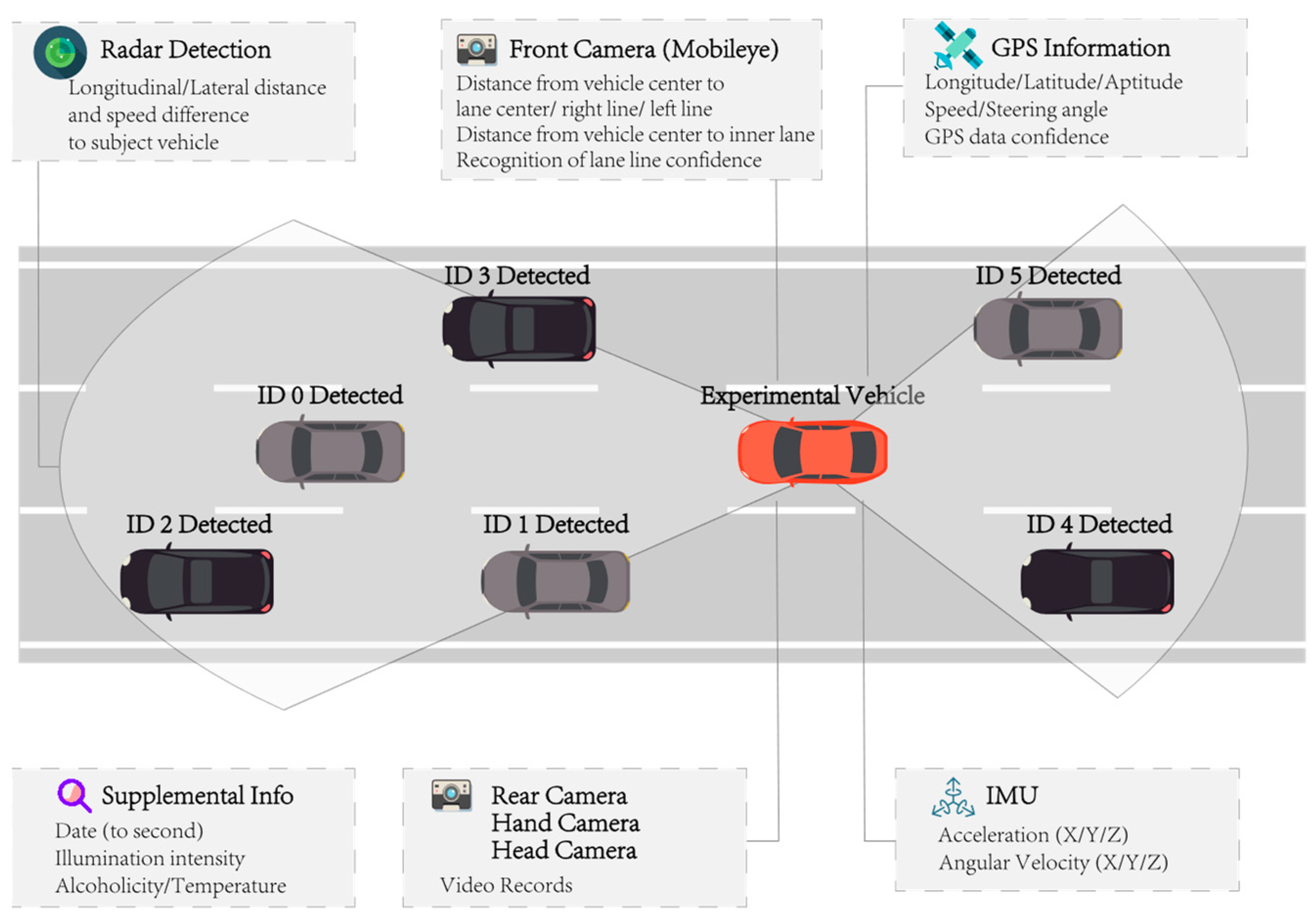
Figure 1 displays the data acquisition system. It consists of a Doppler radar, a triaxial accelerometer, a GPS, and four synchronized cameras. These components work together to capture location data and kinematic information for both the subject vehicle (including speed, longitudinal acceleration, and lateral acceleration) and surrounding vehicles. The data record driving information in time series with up to 86 dimensions. The recording frequency for most data is 10 Hz, while for a few dimensions it is 1 Hz. The radar detects road participants around the vehicle and records at a frequency of 10 Hz. It can record the relative position and speed of up to eight objects at the same time. We determine the vehicle being followed by the subject vehicle based on the relative position relationship. Additionally, the system records any manual operations performed by the driver within the vehicle.
To understand the impact of the driving mode on the modeling accuracy, an extensive comparison of DBDM and DBM is required, which requires enough drivers with enough driving records to be included in the study. In the NDS, natural driving behavior was recorded for a total of 40 Chinese drivers, primarily from the Shanghai metropolitan area, and they were selected at random. The demographic information (gender, driving experience, age) of the 40 drivers is similar to the population of registered drivers in China [
32,
33]. The difference between the distribution of NDD on each dimension and the overall distribution is within 5%. In contrast to the trajectory datasets discussed in
Section 2 and used in CF modeling and driving modes, the NDS offers extensive multi-dimensional data with full spatial-temporal coverage. The NDS not only includes a larger number of participating drivers, but it also provides greater traffic flow facility coverage for each driver than other datasets containing the long-term observations of drivers.
3.2. CF Events Extraction
The dataset was deemed satisfactory for analysis due to minimal noise and missing data. To further enhance the quality of the data, Kalman filtering and cubic spline interpolation techniques were employed for noise reduction and inpainting. An automatic search filter was then utilized to extract CF events based on specific thresholds such as time headway and lateral distance. The extraction criteria were informed by previous research [
34,
35].
Following data extraction, a random sampling methodology was implemented to ensure that the sample accurately reflected general driving behavior. A total of 100 CF events were randomly selected for each driver from a range of traffic flow facilities and conditions. This resulted in a total of 4000 samples collected from the 40 drivers for subsequent analysis, with a total recording time exceeding 2500 min.
4. Methodology
The framework of this study is illustrated in
Figure 2. To solve the problem of the CF data segmentation and clustering according to data structure dependencies, a promising approach, TICC, is applied to the extracted CF events from the NDS. It applies MRFs to encode and match the graphical dependency structure of each subsequence. Then, classic CF models (the IDM and the hybrid IDM-Wiedemann model) are calibrated and validated to compare the performances of the DBM and DMBM.
4.1. CF Events Segmentation and Driving Mode Recognition
4.1.1. Problem Description
As mentioned above, drivers will take different driving modes in the CF process, but the accurate definitions and classification standards for these modes cannot be found in past studies on driving behavior. Driving modes can be viewed as different reoccurring patterns in the time series of the driving behavior of a certain driver, while the time series of CF is usually recorded as multivariate time series data.
We set
as the CF trajectory of
sequential
-dimensional observations, which is expressed as:
where
is the
-th multivariate observation of the trajectory, and
equals 4, which is the number of the key variable in the CF process (acceleration, velocity, gap, and velocity difference).
Discovering driving modes in CF requires a segmentation and clustering process of multivariate time series, which is quite a challenging mathematical problem. Differing from standard time series segmentation, multiple segments can belong to the same cluster, explained as the driving mode in the CF process. On the other hand, driving behavior can be viewed as a continuous relationship in time, thus it is also harder than simple subsequence clustering since each data point cannot be clustered individually (neighboring points are encouraged to belong to the same cluster) [
36]. Additionally, these clusters are required to each present a certain basic CF mode, that is, to be in line with people’s common understanding of basic driving behavior.
4.1.2. Toeplitz Inverse Covariance-Based Clustering (TICC) Method
Therefore, in this research, we adopted a novel unsupervised learning method for the subsequence clustering of multivariate time series to obtain proper driving modes in the CF process for the following calibration, which is called TICC. The discovery of driving modes involves the simultaneous segmentation and clustering of multivariate time series data, and TICC is an innovative method designed to address this problem. This issue is more challenging than conventional time series segmentation because several segments may belong to the same cluster [
37,
38]. However, it is also more complex than the problem of subsequence clustering because individual data points cannot be clustered separately (since neighboring points are encouraged to be in the same cluster) [
39,
40]. Distance-based methods, such as dynamic time warping, are often used to solve these types of problems [
41]. However, they focus more on matching raw values rather than exploring the overall structural consistency of time subsequences by examining the correlations between multidimensional data. TICC was introduced in 2017 and has been widely used in engineering [
42], finance [
43], and medicine [
44] due to its effectiveness. MRFs are used to describe the non-time-varying correlation structure within a window to identify and cluster different subsequences and represent stronger or more complex relationships than simple correlations. TICC alternates between assigning points to clusters, which it accomplishes through dynamic programming, and updating the cluster MRFs, which it does via alternating the direction method of multipliers (ADMM). In comparison with several advanced time series clustering methods, TICC has at least a 41% higher clustering accuracy [
36].
The TICC method avoids clustering each observation, since for the CF process, an isolated observation may tell an instantaneous state of the CF pair. The TICC cluster short subsequence of size
(
), consisting of observations
,…,
, was concatenated into an
-dimensional subsequence called
. Then, a new sequence was formed and named
, from
to
, on which the clustering process was applied. An
-dimensional subsequence
allows more time-varying information to be analyzed and clustered in the driving process. Meanwhile, the adjacent subsequences are encouraged to be clustered into the same cluster, which is called temporal consistency [
36].
Rather than choosing simple correlation-based models, the segmenting and clustering of the multivariate time series is based on Markov random fields (MRFs), which is a multilayer correlation network which encodes the structural relationships between data of different dimensions, as shown in
Figure 3. It not only considers the interdependencies of all dimensions of
; the dependency of neighbor points is also taken into account. The Toeplitz matrix
defines the MRFs edge structure using a Gaussian inverse covariance instead of covariance for the computational advantages as the result of a tendency of being sparse and preventing overfitting.
One challenge associated with the TICC approach is addressing the assignment problem of allocating data points to one of the K clusters and determining the assignment sets
with
. Additionally, the algorithm must update cluster parameters
based on previously calculated assignment mappings. This optimization problem can be expressed as follows:
where
represents the set of symmetric block Toeplitz
matrices and serves as an additional constraint for constructing MRFs to ensure the time-invariant property of each cluster. The first expression
denotes an additional sparsity constraint based on the Hadamard product of the inverse covariance matrix with the regularization parameter
. The second component,
, specifies the core optimization problem of fitting cluster parameters given the assignment set
(log likelihood). The indictor function
is checks the temporal consistency, that is, whether adjacent data points belong to the same cluster. If two observations are consecutive but assigned to different clusters
, there will be a penalty
.
There are two key input parameters for the TICC algorithm: the window size
and the number of the clusters
. The TICC does not cluster each data point
individually, it instead clusters short subsequences from
to
. The size of the Toeplitz
matrices determines whether it is too short to contain the complete MRF structure of each cluster, and it is too long to choose a segment boundary or disobey the time-invariance as well. To effectively use this algorithm, we refer to Hallac, Vare, Boyd, and Leskovec [
36] and set the window size to 10 since they suggested that when the window size is bounded between 4 and 15, the clustering result of the car data would be reliable and robust. Another key parameter is
. Since we do not have any proper precedent for CF mode extraction, we will test different values of
K according to the behavior reproduction performance as well as the Bayesian information criterion (BIC).
The TICC problem is a combinatorial optimization problem, which has two coupled non-convex problems to search the optimized cluster parameter
and the cluster assignments
. Since it is difficult to solve global optimization, an expectation–maximization (EM)-like algorithm is applied, which constantly and alternately assign
with
determined and update
with
determined. For the solution process of the TICC, please refer to
Appendix A. A brief outline of TICC clustering is shown in Algorithm 1.
| Algorithm 1 Brief outline of TICC clustering |
| 1: | initialization Cluster parameters and assignments |
| 2: | repeat |
| 3: | E-step: Assign points to clusters → |
| 4: | M-step: Update cluster parameters → |
| 5: | until Stationarity. |
| | return (, ) |
4.2. CF Model Calibration and Validation Based on Driving Modes
In a conventional way, the potential intra-driver variance in a CF event is actually “averaged”. Given the recognized driving modes in CF events, the CF model can be calibrated based on driving modes rather than drivers to further understand the impact of this neglect. This subsection describes the calibration and validation of three typical CF models through the extracted empirical CF events. The selected CF models are first introduced, then a standardized calibration and validation process is explained.
4.2.1. Investigated CF Models
- 1.
Intelligent Driver Model (IDM)
We have thoroughly investigated and compared the CF model performances in our previous study [
1]; the IDM was validated as the best in several commonly used models for its superiority in CF behavioral reproduction, and therefore, IDM was also chosen to be the main CF model in this study. The IDM will be calibrated both from DBM and DMBM perspectives.
The IDM is a widely recognized CF model that utilizes the concept of desired measures. Unlike the Gipps model, the IDM possesses the capability to intelligently select CF modes, facilitating a smooth transition between free-flow and CF conditions. Additionally, each parameter in the IDM represents a distinct aspect of driving behavior, rendering it more parsimonious and easier to calibrate. The IDM can be defined as:
where
is the maximum acceleration,
is the comfort deceleration,
is the desired velocity,
is the relative distance,
is the desired spacing, and
is the minimum distance when at a standstill.
- 2.
Wiedemann model
The logic of CF that the CF interaction can be divided by perceptual thresholds was proposed by Wiedemann of Karlsruhe University. The Wiedemann model is recognized as a quintessential psycho-physical CF model that incorporates human factors to more accurately replicate realistic driving behavior, of which the CF logic is shown in
Figure 4. The CF process is divided by different thresholds with a certain shape, and the subject vehicle takes different acceleration maneuvers. In this study, we utilized the Wiedemann 99 model, an updated version of the original Wiedemann model that accounts for both driver characteristics and driving modes. This model has recently gained popularity in both academic research and practical applications for its ability to accurately simulate car-following behavior. The model was calibrated individually for each driver in our study. For a detailed formulation, please refer to the literature [
45,
46].
- 3.
Hybrid Wiedemann-IDM model
Some researchers have argued that the sub-models in the Wiedemann model negatively affect the performance rather than the driving mode division part and have thus proposed a hybrid Wiedemann-IDM model [
21]. That is, the original Wiedemann model is altered by replacing the acceleration equations in different CF modes (free-flow mode, closing-in mode, following mode, and emergency braking mode, as shown in
Figure 4) with the most adaptable CF model so far, the IDM. These IDMs of each CF regime of the Wiedemann will be calibrated and given a set of parameters for each of the modes in this hybrid model. The reason why we introduce this hybrid model is to figure out (1) whether it is the acceleration equations or the driving modes that weaken the performance of the Wiedemann model, and (2) whether the objective rule-based division of driving modes in the Wiedemann can reasonably identify different modes in human CF process.
4.2.2. CF Calibration
The evaluation of the calibration results is crucial for determining the capability of a CF model to accurately replicate real-world driving behavior, minimizing discrepancies between simulated data and actual observations within the parameter space being searched. The validation process is usually responsible for the effectiveness of model parameter calibration and parameter generalization, for example, testing how whether a set of parameters can fit well the other CF events of a certain driver.
K-fold cross-validation is a commonly used model evaluation method. It divides the dataset into five parts and uses four of them as training data and the remaining one as test data each time. We adopted five-fold cross validation in this study, which allows for five rounds of training and testing, with the average value taken as the performance evaluation of the model, as shown in
Figure 5. This method can effectively avoid overfitting and better evaluate the model’s performance on unknown data. For each driver involved in the calibration, 80 of the 100 events were for calibration and the other 20 events were for validation, iterating in turn. The average error on the validation data was used to compare the performance of the investigated models.
To ensure the accuracy of comparison results in the calibration process, we followed a specific protocol. First, our objective function was defined as the deviation between simulated and observed spacing measures [
47,
48], which has been demonstrated to be a reliable metric in previous studies [
49,
50]. Following an in-depth analysis of the objective function presented in [
51], we employed the root mean square normalized error (RMSNE) as a measure of the relative error. This has been shown to be effective in previous studies [
48,
52], defined as:
where
and
are the
th observed spacing and simulated spacing, respectively, with
ranging from 1 to
.
To address the constrained nonlinear optimization problem in the calibration process, a genetic algorithm (GA) was employed in our empirical experiments. The effectiveness of GA was previously validated in the literature [
1,
9]. To ensure fast convergence and realistic kinematics, we set the bounds and initial searching values of the CF model parameters based on the values reported in previous studies [
21,
24,
49].
Table A1 summarizes these values. During the calibration of the DBM, a set of parameters achieving global optimization on the error of reproducing the driver’s CF events set is assigned to each driver. Similarly, during the calibration of the DMBM, each mode is assigned a set of parameters. The obtaining of the results of the DMBM involves a two-step calibration process. First, TICC was used to obtain the driving-mode labels of each time step (the labels were generated for each candidate value of the number of undetermined K). Then, in the calibration process, the objective function (which simulates CF trajectories and calculates calibration errors) dynamically chooses different sets of parameters based on the driving mode labels, as shown in
Figure 6. After calibration, the optimal parameters can be solved.
In an effort to attain the global optimum, we conducted the optimization procedure ten times for each car-following event. The set of parameters that yielded the lowest RMSNE was recorded. Since the optimization process requires a large population size in GA, while the searching spacing of the parameters of the hybrid model or the DMBM model is much larger than the IDM, we utilized a high-performance server to solve the calibration in parallel. Its CPU is AMD EPYC 7H12 with 64 cores and 128 threads.
5. Results
In this section, the results of the two CF behavior modeling pathways (driving-mode-based or driver-based) are presented. First, we compared the CF model performance under different settings of the clustering number, and then attempted to determine the most proper value and provide a qualitative interpretation of physical meanings to each mode. Second, the CF model performances under different CF modeling views are compared.
5.1. Segmentation and Clustering of CF Behavior
So far, there is no ground truth of specific driving behavior segmentation for the optimization of CF modeling. The TICC algorithm is unsupervised, and the number of clusters
for the next CF modeling is undetermined. Therefore, the Bayesian information criterion (BIC) was utilized to determine the appropriate value of
, which is a standard criterion for model selection among a finite set of models. Generally, models with a lower BIC score are considered more favorable. Meanwhile, for the CF model IDM, of which the number of parameters is five, the parameter quantity for each CF model under the segmentation of
clusters is five times
. Therefore, for efficient CF modeling, the value of K is expected to be as small as possible while achieving ideal model accuracy. In this study, we hoped to achieve a balance between the BIC of the segmentation, the number of clusters, and the CF model’s performance. We tested the IDM’s performance, calculated the BICs on different K values (from 2 to 10), and the results are presented in
Figure 7.
As shown in
Figure 7, BIC increases with the value of
and stabilizes after seven, while the CF modeling error decreases sharply before four and then reaches a slow decline in volatility. Therefore, the numbers of
, four or five, are potential candidates since their RMSNEs have reached an ideal range (under 0.22, which have been clearly smaller than the errors of driver-based modeling). Meanwhile, both the BIC and RMSNE values of
value five is lower than four with only five parameters added, thus we chose five as the proper
value in this study. The calibrated IDM parameters for each mode are listed in
Table A2.
Then, based on the current
value, the segmentations of CF samples are presented in
Figure 8. Benefiting from time-window-based clustering and its emphasis on temporal consistency by function
, different phases in a CF event can avoid fragmentation well. Furthermore, in order to understand the relationship between clusters and CF behaviors, that is, to determine whether different clusters can represent different CF modes, we manually checked more than 100 segmented events and attempted to qualitatively distinguish and interpret the physical meaning of each cluster, and the summary results are shown in
Table 1. This shows that the application of data-driven TICC can indeed divide different CF modes well. Please note that this interpretation does not mean that these CF modes can be simply divided based on the variable features in the table or additional thresholds, as the variable relationships inherent in the TICC are complex and difficult to be described quantitatively.
5.2. Comparative Results
Before we compare the calibration errors, it should be clear what the quantities of the parameters for the CF modeling are. For the DBM, the calibration process must be conducted once for every driver so that the CF model can well replicate the inter-driver heterogenous behavior of each driver. Thus, the number of parameters for the DBM are times the number of model parameters, where represents the number of drivers. For example, 200 parameters are needed to be calibrated for 40 drivers using IDM, while 440 parameters are needed when using Wiedemann. Meanwhile, the DBDM is not related to the number of drivers because it is determined by the kinds of segmented driving modes, so the number of parameters for the DMBM is times five, where represents the number of driving modes. In this study, this means that 25 parameters are needed for the IDM and 55 are needed for the Wiedemann.
First, on the comparison of the calibration errors of three DBM models, which is shown in
Figure 9a, the IDM shows a clear advantage over the Wiedemann model, reaching 15%, but the error of the IDM is higher than that of the hybrid model. Considering that the parameters of the hybrid model are four times more than those of IDM, this reduction in error was expected. Meanwhile, the calibration error of the DBM is significantly higher than that of the DMBM. The latter reduces the error by 13.12%. This indicates that DMBM could better reproduce CF behavior with much less parameters than DBM.
When examining the results more deeply, we found that in the five-fold cross-validation process, the mean validation error of the DBM is clearly higher than its calibration error (over 13%), while this does not exist in the DMBM (only 4.53% error growth), as shown in
Figure 9b. This may indicate another advantage of the DMBM, that is the better portability or practicality. The parameters from the DBM may specialize in specific CF events, but the existing behavior variance between different events, even from the same driver, makes these parameters invalid to some extent, which can be viewed as a kind of “overfitting”.
6. Discussion
This study introduces and investigates a new perspective in CF modeling, that is, modeling CF driving modes rather than for an individual human driver or an entire CF event (or a CF period in some studies). Although we have known and verified many times that the CF behavior of human beings is not static in the driving process, this study is the first in-depth study to discover the driving modes of the CF process and the improvements that can be achieved by modeling CF driving modes, with the help of the application of a novel approach in the clustering of multivariate time series data. This study also benefits from large-scale naturalistic driving data, which provides sufficient and diverse samples of drivers’ CF behavior.
In past research, a “consensus” has gradually formed that well-constructed driver-based models, which can reproduce CF trajectories better than those of driving-status-based models, such as the Wiedemann model. To some extent, these kinds of investigation results may lead to an emphasis on the inter-driver or inter-CF-period differences rather than intra-driver or intra-period variances in future CF modeling research. Higgs et al. proposed that the imprecise sub-models in Wiedemann lead to unsatisfactory results and pointed out a pathway to combine the state division of the Wiedemann with other CF models. That is why we also introduced a Wiedemann-IDM model for comparison. The result shows that this combination can be better than the original Wiedemann model, even IDM, but the error improvement of the IDM is relatively limited. This drives us to think about another aspect, that being how much potential improvement there could be if driving modes are well partitioned and modeled.
Therefore, we introduced a novel and recent unsupervised multivariate time series clustering approach. The large accuracy increase in the DMBM has proved the effectiveness of the adopted clustering method. By using the graphical dependency structure of each subsequence, the algorithm can dig out the underlying multidimensional time-invariant relationship that cannot be expressed and distinguished using a simple threshold division. Meanwhile, once a TICC model has been trained, it can be applied to a new multivariate CF time series to predict clusters, which will not reduce applicability due to the inability to provide threshold division.
The results confirm our initial conjecture, which is that modeling accuracy can be improved by modeling several shared underlying driving modes in the CF process. This is encouraging since it has been verified with only five driving mode classifications. As mentioned above, some researchers [
7] have attempted to preliminary verify a conclusion, but on a scale of up to 30 classifications and with only 20 drivers, and the parameter number used for the DMBM is far more than the DBM (120 versus 80, based on the 4-parameter GHR model). That means that the CF event will be too fragmented, and it is hard to determine whether the accuracy improvement is due to reasonable behavior segmentation or that more parameters are used to describe shorter segments. Meanwhile, based on our experience in CF research, an enormous number of parameters will bring about an extreme increase in the calibration time, which is very negative for the practice of CF modeling. In contrast, we proved that only 25 parameters could well describe the CF behavior from 30 drivers rather than 120 parameters from the DBM. In a word, the error caused by the neglect of behavioral differences between driving modes has been underestimated before, and it is promising and necessary to involve targeted driving modes modeling in future CF modeling practices.
We expect our model to be mainly applied in two aspects, as mentioned in the introduction: accurate traffic flow simulation and ADASs on intelligent vehicles. Both require a better understanding of human driver behavior. In traffic flow simulation, traditional approaches assign uniform behavioral parameters to all vehicles. Transitioning from individual vehicles to driving-mode-based modeling can increase heterogeneity while avoiding difficulties in parameter generation [
53]. In intelligent vehicle applications, one potential application is in driver identification. Based on our proposed methods, the driving mode distribution or transition characteristics of each driver can be quantitatively calculated to achieve driver identification [
54]. This is very useful for vehicles with intelligent driving assistance that value in-car privacy protection. Another application is to help drivers better drive the vehicle during CF in ACC, with more human-like intra-driver differences in the driving process.
Other than the novelty and strengths of this proposal, there are a few limitations. First, the combination of driving modes and individual differences was ignored because it is a big computational challenge to calibrate 25 parameters. A future study will enable each driver to have their own parameters for different driving modes, which can help advanced driver assistance systems select more personalized parameters for drivers. Second, this study did not explore the quantitative characteristics or the identification of each driving mode. Since each driving mode is identified by the complex TICC method, which involves the spatiotemporal relationships between multiple variables, it may be unrealistic to determine the mathematical expression of each mode in this study. In the future, deep learning models should be used to consider the long- and short-term spatiotemporal correlations contained in each driving mode.
7. Conclusions
Due to the importance of CF behavior in both macro traffic flow management or micro effective safety functions in ADASs, CF behavior has been extensively investigated to reproduce more realistic human driving trajectories. However, deep knowledge of driving modes in CF and the behavioral differences between modes is lacking, meaning there needs to be a further improvement in the CF modeling accuracy. This study adopted a novel MRF-based time series clustering method to solve the segmentation and clustering of driving modes from massive multivariate naturalistic driving data. A comprehensive comparison of different CF modeling perspectives (DBM and DMBM) is conducted, benefiting from the long-term behavior records of more than 40 drivers.
Using the TICC method, five types of CF driving modes are discovered, which can significantly increase the accuracy in reproducing CF behavior with a relatively low clustering BIC criterion. These five data-driven classifications are understandable and basically correspond to the different steps in the human CF process, namely, continuous distance, continuous approach, high-speed stable follow-up, low-speed close-range stable follow-up, and vulgar long-distance follow-up. These five modes describe structural repetitions in human operational behavior.
Precise CF modeling: Based on the determined CF modes, the driving-mode-based IDM performed better than the driver-based IDM and the hybrid Wiedemann-IDM model, leading by 17.49% and 13.59%, respectively. The lower error compared to the hybrid model further affirms the effect of the TICC algorithm on the recognition of driving modes rather than the mode-division part in the Wiedemann.
Efficient CF modeling: This is an impressive improvement by the DMBM with far fewer parameters, demonstrating how much potential DMBM has if the driving modes in the CF process can be well recognized. It does not require specific modeling for each driver, whose parameter set is likely not transferable to describe the CF behavior of the other drivers. Meanwhile, the error of the DMBM during the validation process does not increase much compared to that of the calibration, indicating its good transferability for future applications.
This study answered an essential question of how the different modes in the CF affect the CF modeling accuracy. By doing so, it expanded the understanding of human CF behavior. On the one hand, it offered an objective perspective on the basic modes involved in the human CF process. On the other hand, it explains the importance of integrating intra-driver variance, especially the behavioral differences between CF modes, into the consideration of the development of CF modeling and personalized advanced driving assistance systems (ADASs). Furthermore, the clustering results of this study may provide support for potential driver recognition since CF behavior can be viewed as a different mode combination of different drivers.
However, we should note that this is a preliminary heuristic study on the DMBM. In this study, we focused on discovering the existence of CF modes and their impact on behavior modeling but did not deeply explore the spatiotemporal connection or mathematical quantitative expressions between different modes, which is the direction of our next work.
Author Contributions
Conceptualization, D.Z., H.R. and L.Y.; methodology, D.Z. and H.R.; resources, J.S.; data curation J.W. and J.S.; writing, D.Z.; supervision, J.S. and L.Y.; funding acquisition, J.S. All authors have read and agreed to the published version of the manuscript.
Funding
This research is jointly sponsored by the National Natural Science Foundation of China (52125208), the National Natural Science Foundation of China (52232015), and the Zhejiang Lab Open Research Project (NO.2021NL0AB02).
Institutional Review Board Statement
The study was quite rigorous in guaranteeing the anonymity of participated drivers in NDS. The NDS project obtained informed consent from the participants, informing them that the data would be used only for academic research and would not have any negative impact on them.
Informed Consent Statement
Informed consent was obtained from all subjects involved in the study.
Data Availability Statement
Restrictions apply to the availability of these data since data were obtained from multi-party cooperation.
Conflicts of Interest
The authors declare no conflict of interest.
Appendix A. A Solving Process of the TICC
Appendix A.1. Expectation Part: Cluster Assignment
At this step, TICC assigns observations to the given clusters. At the very start, k-means is adopted to obtain prior distribution for the initial assignment and then the initial cluster parameter
can be obtained. With fixing
, T subsequences is assigned to K clusters according to the optimization:
to maximize the two objectives, the log likelihood
and the temporal consistency
are used, which determines how possible adjacent points belong to the same cluster. The solving process is a dynamic programming approach. The process involves finding the path with the minimum cost from timestamp 1 to T, where the cost of a node is the negative log likelihood of the point being assigned to a particular cluster. Algorithm A1 provides a pseudo code for this process.
| Algorithm A1 Solving the cluster assignment |
| 1: | given , negative log likelihood of point assigned to cluster |
| 2: | initialize prev_cost = list of zeros |
| 3: | curr_cost = list of zeros |
| 4: | prev_path = list of K empty lists |
| 5: | curr_path = list of K empty lists |
| 6: | for = 1 to do |
| 7: | for = 1 to do |
| 8: | min_index = index of minimum value of prev_cost |
| 9: | if prev_cost[minIndex] + > prev_cost[] then |
| 10: | curr_cost[] = PrevCost[] − |
| 11: | curr_path[] = PrevPath[].append[] |
| 12: | else |
| 13: | curr_cost[j] = prev_cost[minindex] + − |
| 14: | curr_path[j] = prev_path[minindex].append[j] |
| 15: | prev_cost = curr_cost. |
| | prev_path = curr_path |
| | final_min_index = index of minimum value of curr_cost |
| | final_path = curr_path[final_min_index] |
| | return final_path. |
Appendix A.2. Maximization Part: Updating Cluster Parameters
With fixing cluster assignments
, the next task is to update the inverse covariance matrices of the clusters. Since the temporal consistency
is mainly connected to the problem A.1, the optimization problem can be simplified as:
In addition, since in this part there is no dependency on previous and cross-connected results of other clusters in [
55], the updates can be conducted in parallel [
36]. The negative log likelihood in terms of each
can be expressed as:
where
represent the number of the points assigned to cluster
;
and
are the determinant and the trace of a matrix, respectively;
is the empirical covariance of the random sample, which is open adopted to approximate the true covariance matrix Σ of a stochastic problem [
56]; and
is a constant. Therefore, the update representation of this optimization problem is expressed as:
Hallac, Vare, Boyd, and Leskovec [
36] defined this optimization problem as the Toeplitz graphical lasso, and as a variation of the classical graphical lasso problem [
57]. It is required to solve an individual Toeplitz graphical lasso for every cluster at each iteration. The alternating direction method of multipliers (ADMM) was applied to solve this problem as a well-performed algorithm in solving related large-scale convex problems [
58]. In order to construct the ADMM-friendly form, a consensus variable
is introduced to reconstruct the problem as:
where
allows the optimization to be separated into two sub-problems. ADMM approximates the result of the initial problem alternately, updating one variable with the others staying fixed. For a detailed calculation process, please refer to [
36,
58].
Appendix B. Calibration Settings and Results
This part lists the bounds and initial searching values of the parameters in
Table A1 and the calibrated parameters for each mode in
Table A1.
Table A1.
The bounds and initial searching values of parameters for calibration.
Table A1.
The bounds and initial searching values of parameters for calibration.
| Model | Parameter | Description of Parameter | Bounds | Initial
Searching Value |
|---|
| IDM model | | Gap at standstill | [0.1, 10] | 2.6 |
| Desired time headway | [0.1, 5] | 1.5 |
| Maximum acceleration | [0.1, 5] | 1.5 |
| Maximum deceleration | [0.1, 5] | 1.5 |
| Desired speed | [10, 50] | 30.0 |
| Wiedemann 99 model | | Standstill gap | [0.1, 10] | 1 |
| Headway time | [0.1, 5] | 1.5 |
| Following variation | [0.1, 10] | 5 |
| Threshold for entering “following” | [−20, 0] | −10 |
| Negative “following” threshold | [−5, 0] | −2.5 |
| Positive ‘following’ threshold | [0.1, 5] | 2.5 |
| Speed dependency of oscillation | [0.1, 20] | 10 |
| Oscillation acceleration | [−1, 1] | 0 |
| Standstill acceleration | [0.1, 8] | 4 |
| Acceleration at 80 km/h | [0.1, 8] | 4 |
| Desired speed | [20, 40] | 35 |
Table A2.
The calibrated parameters for each driving mode.
Table A2.
The calibrated parameters for each driving mode.
| | | | | | |
|---|
| Mode 0 | 9.9998 | 0.2876 | 1.6982 | 2.8065 | 42.9453 |
| Mode 1 | 4.5527 | 0.4834 | 1.9633 | 0.3222 | 38.0056 |
| Mode 2 | 7.7071 | 0.2242 | 0.6345 | 0.1010 | 45.1651 |
| Mode 3 | 3.5765 | 2.7590 | 0.9904 | 0.1007 | 41.1865 |
| Mode 4 | 9.9998 | 0.1008 | 0.3539 | 2.6250 | 49.9999 |
References
- Zhang, D.; Chen, X.; Wang, J.; Wang, Y.; Sun, J. A comprehensive comparison study of four classical car-following models based on the large-scale naturalistic driving experiment. Simul. Model. Pract. Theory 2021, 113, 102383. [Google Scholar] [CrossRef]
- Sun, J.; Zheng, Z.; Sun, J. Stability analysis methods and their applicability to car-following models in conventional and connected environments. Transp. Res. Part B Methodol. 2018, 109, 212–237. [Google Scholar] [CrossRef]
- Higatani, A.; Saleh, W. An investigation into the appropriateness of car-following models in assessing autonomous vehicles. Sensors 2021, 21, 7131. [Google Scholar] [CrossRef] [PubMed]
- Halim, Z.; Kalsoom, R.; Bashir, S.; Abbas, G. Artificial intelligence techniques for driving safety and vehicle crash prediction. Artif. Intell. Rev. 2016, 46, 351–387. [Google Scholar] [CrossRef]
- Halim, Z.; Rehan, M. On identification of driving-induced stress using electroencephalogram signals: A framework based on wearable safety-critical scheme and machine learning. Inf. Fusion 2020, 53, 66–79. [Google Scholar] [CrossRef]
- Chen, X.; Sun, J.; Ma, Z.; Sun, J.; Zheng, Z. Investigating the long-and short-term driving characteristics and incorporating them into car-following models. Transp. Res. Part C Emerg. Technol. 2020, 117, 102698. [Google Scholar] [CrossRef]
- Higgs, B.; Abbas, M. Segmentation and clustering of car-following behavior: Recognition of driving patterns. IEEE Trans. Intell. Transp. Syst. 2014, 16, 81–90. [Google Scholar] [CrossRef]
- Van Hinsbergen, C.; Schakel, W.; Knoop, V.; van Lint, J.; Hoogendoorn, S. A general framework for calibrating and comparing car-following models. Transp. A Transp. Sci. 2015, 11, 420–440. [Google Scholar] [CrossRef]
- Chen, C.; Li, L.; Hu, J.; Geng, C. Calibration of MITSIM and IDM car-following model based on NGSIM trajectory datasets. In Proceedings of the 2010 IEEE International Conference on Vehicular Electronics and Safety, Qingdao, China, 15–17 July 2010; pp. 48–53. [Google Scholar]
- Lu, X.-Y.; Skabardonis, A. Freeway traffic shockwave analysis: Exploring the NGSIM trajectory data. In Proceedings of the 86th Annual Meeting of the Transportation Research Board, Washington, DC, USA, 21–25 January 2007. [Google Scholar]
- Coifman, B.; Li, L. A critical evaluation of the Next Generation Simulation (NGSIM) vehicle trajectory dataset. Transp. Res. Part B Methodol. 2017, 105, 362–377. [Google Scholar] [CrossRef]
- Kurtc, V. Studying car-following dynamics on the basis of the HighD dataset. Transp. Res. Rec. 2020, 2674, 813–822. [Google Scholar] [CrossRef]
- Saifuzzaman, M.; Zheng, Z. Incorporating human-factors in car-following models: A review of recent developments and research needs. Transp. Res. Part C Emerg. Technol. 2014, 48, 379–403. [Google Scholar] [CrossRef]
- Chandler, R.E.; Herman, R.; Montroll, E.W. Traffic dynamics: Studies in car following. Oper. Res. 1958, 6, 165–184. [Google Scholar] [CrossRef]
- Lee, G. A generalization of linear car-following theory. Oper. Res. 1966, 14, 595–606. [Google Scholar] [CrossRef]
- Ahmed, K.I. Modeling Drivers’ Acceleration and Lane Changing Behavior; Massachusetts Institute of Technology: Cambridge, MA, USA, 1999. [Google Scholar]
- Kometani, E. Dynamic behavior of traffic with a nonlinear spacing-speed relationship. In Theory of Traffic Flow, Proceedings of the Symposium on the Theory of Traffic Flow (GM), Detroit, MI, USA, 7–8 December 1959; Transportation Research Board: Washington, DC, USA, 1959; pp. 105–119. [Google Scholar]
- Newell, G.F. Nonlinear effects in the dynamics of car following. Oper. Res. 1961, 9, 209–229. [Google Scholar] [CrossRef]
- Gipps, P.G. A behavioural car-following model for computer simulation. Transp. Res. Part B Methodol. 1981, 15, 105–111. [Google Scholar] [CrossRef]
- Helly, W. Simulation of Bottlenecks in Single-Lane Traffic Flow; Scientific Research Publishing: Wuhan, China, 1959. [Google Scholar]
- Higgs, B.J. Application of Naturalistic Truck Driving Data to Analyze and Improve Car Following Models; Virginia Tech: Blacksburg, VA, USA, 2011. [Google Scholar]
- Higgs, B.; Abbas, M.; Medina, A. Analysis of the Wiedemann car following model over different speeds using naturalistic data. In Proceedings of the 3rd International Conference on Road Safety and Simulation, Indianapolis, IN, USA, 14–15 September 2011; pp. 1–22. [Google Scholar]
- Huang, X.; Sun, J.; Sun, J. A car-following model considering asymmetric driving behavior based on long short-term memory neural networks. Transp. Res. Part C Emerg. Technol. 2018, 95, 346–362. [Google Scholar] [CrossRef]
- Wang, H.; Wang, W.; Chen, J.; Jing, M. Using trajectory data to analyze intradriver heterogeneity in car-following. Transp. Res. Rec. 2010, 2188, 85–95. [Google Scholar] [CrossRef]
- Lin, Q.; Zhang, Y.; Verwer, S.; Wang, J. MOHA: A multi-mode hybrid automaton model for learning car-following behaviors. IEEE Trans. Intell. Transp. Syst. 2018, 20, 790–796. [Google Scholar] [CrossRef]
- Müller, M. Dynamic time warping. In Information Retrieval for Music and Motion; Springer: Berlin/Heidelberg, Germany, 2007; pp. 69–84. [Google Scholar]
- Farhi, N.; Haj-Salem, H.; Lebacque, J.-P. Multianticipative piecewise-linear car-following model. Transp. Res. Rec. 2012, 2315, 100–109. [Google Scholar] [CrossRef]
- Dodge, S.; Laube, P.; Weibel, R. Movement similarity assessment using symbolic representation of trajectories. Int. J. Geogr. Inf. Sci. 2012, 26, 1563–1588. [Google Scholar] [CrossRef]
- Gionis, A.; Mannila, H. Finding recurrent sources in sequences. In Proceedings of the Seventh Annual International Conference on Research in Computational Molecular Biology, Berlin, Germany, 10–13 April 2003; pp. 123–130. [Google Scholar]
- Zolhavarieh, S.; Aghabozorgi, S.; Teh, Y.W. A review of subsequence time series clustering. Sci. World J. 2014, 2014, 312521. [Google Scholar] [CrossRef] [PubMed]
- Keogh, E.; Lin, J. Clustering of time-series subsequences is meaningless: Implications for previous and future research. Knowl. Inf. Syst. 2005, 8, 154–177. [Google Scholar] [CrossRef]
- Traffic Administration Bureau of the Ministry of Public Security, Ministry of Public Security, China. The Number of Drivers in Our Country Is Growing Rapidly, with an Average Annual Increase of 25 Million People. The Total Number of Drivers Exceeds 500 Million, Ranking First in the World. Available online: https://app.mps.gov.cn/gdnps/pc/content.jsp?id=8794518 (accessed on 20 April 2023).
- Traffic Administration Bureau of the Ministry of Public Security, Ministry of Public Security, China. In 2021, the Number of Motor Vehicles in the Country Reached 395 Million, and the Number of New Energy Vehicles Increased by 59.25% Year-on-Year. Available online: https://app.mps.gov.cn/gdnps/pc/content.jsp?id=8322369 (accessed on 20 April 2023).
- LeBlanc, D.J.; Bao, S.; Sayer, J.R.; Bogard, S. Longitudinal driving behavior with integrated crash-warning system: Evaluation from naturalistic driving data. Transp. Res. Rec. 2013, 2365, 17–21. [Google Scholar] [CrossRef]
- Sun, J.; Zhang, Y.-h.; Wang, J.-h. Detecting Distraction Behavior of Drivers Using Naturalistic Driving Data. China J. Highw. Transp. 2020, 33, 225. [Google Scholar]
- Hallac, D.; Vare, S.; Boyd, S.; Leskovec, J. Toeplitz inverse covariance-based clustering of multivariate time series data. In Proceedings of the 23rd ACM SIGKDD International Conference on Knowledge Discovery and Data Mining, Halifax, NS, Canada, 13–17 August 2017; pp. 215–223. [Google Scholar]
- Hallac, D.; Nystrup, P.; Boyd, S. Greedy Gaussian segmentation of multivariate time series. Adv. Data Anal. Classif. 2019, 13, 727–751. [Google Scholar] [CrossRef]
- Himberg, J.; Korpiaho, K.; Mannila, H.; Tikanmaki, J.; Toivonen, H.T. Time series segmentation for context recognition in mobile devices. In Proceedings of the 2001 IEEE International Conference on Data Mining, San Jose, CA, USA, 29 November–2 December 2001; pp. 203–210. [Google Scholar]
- Begum, N.; Ulanova, L.; Wang, J.; Keogh, E. Accelerating dynamic time warping clustering with a novel admissible pruning strategy. In Proceedings of the 21th ACM SIGKDD International Conference on Knowledge Discovery and Data Mining, Sydney, NSW, Australia, 10–13 August 2015; pp. 49–58. [Google Scholar]
- Smyth, P. Clustering sequences with hidden Markov models. Adv. Neural Inf. Process. Syst. 1996, 9. [Google Scholar]
- Berndt, D.J.; Clifford, J. Using dynamic time warping to find patterns in time series. In Proceedings of the KDD Workshop, Seattle, WA, USA, 31 July–1 August 1994; pp. 359–370. [Google Scholar]
- Dai, L.; Li, Y.; Zhang, M. Detection of Operator Fatigue in the Main Control Room of a Nuclear Power Plant Based on Eye Blink Rate, PERCLOS and Mouse Velocity. Appl. Sci. 2023, 13, 2718. [Google Scholar] [CrossRef]
- Ouyang, H.; Wei, X.; Wu, Q. Stock index pattern discovery via toeplitz inverse covariance-based clustering. Rom. J. Econ. Forecast. 2020, 23, 58–72. [Google Scholar]
- Yang, X. Multi-series Time-aware Sequence Partitioning for Disease Progression Modeling. In Proceedings of the 30th International Joint Conference on Artificial Intelligence (IJCAI), Montreal-Themed Virtual Reality, 19–26 August 2021. [Google Scholar]
- Durrani, U.; Lee, C. Calibration and validation of psychophysical car-following model using driver’s action points and perception thresholds. J. Transp. Eng. Part A Syst. 2019, 145, 04019039. [Google Scholar] [CrossRef]
- Anil Chaudhari, A.; Srinivasan, K.K.; Rama Chilukuri, B.; Treiber, M.; Okhrin, O. Calibrating Wiedemann-99 model parameters to trajectory data of mixed vehicular traffic. Transp. Res. Rec. 2022, 2676, 718–735. [Google Scholar] [CrossRef]
- Soria, I.; Elefteriadou, L.; Kondyli, A. Assessment of car-following models by driver type and under different traffic, weather conditions using data from an instrumented vehicle. Simul. Model. Pract. Theory 2014, 40, 208–220. [Google Scholar] [CrossRef]
- Punzo, V.; Simonelli, F. Analysis and comparison of microscopic traffic flow models with real traffic microscopic data. Transp. Res. Rec. 2005, 1934, 53–63. [Google Scholar] [CrossRef]
- Treiber, M.; Kesting, A. Microscopic calibration and validation of car-following models—A systematic approach. Procedia-Soc. Behav. Sci. 2013, 80, 922–939. [Google Scholar] [CrossRef]
- Punzo, V.; Montanino, M. Speed or spacing? Cumulative variables, and convolution of model errors and time in traffic flow models validation and calibration. Transp. Res. Part B Methodol. 2016, 91, 21–33. [Google Scholar] [CrossRef]
- Punzo, V.; Ciuffo, B.; Montanino, M. Can results of car-following model calibration based on trajectory data be trusted? Transp. Res. Rec. 2012, 2315, 11–24. [Google Scholar] [CrossRef]
- Ciuffo, B.; Punzo, V. Verification of traffic micro-simulation model calibration procedures: Analysis of goodness-of-fit measures. In Proceedings of the 89th Annual Meeting of the Transportation Research Record, Washington, DC, USA, 10–14 January 2010. [Google Scholar]
- Kim, I.; Kim, T.; Sohn, K. Identifying driver heterogeneity in car-following based on a random coefficient model. Transp. Res. Part C Emerg. Technol. 2013, 36, 35–44. [Google Scholar] [CrossRef]
- Halim, Z.; Kalsoom, R.; Baig, A.R. Profiling drivers based on driver dependent vehicle driving features. Appl. Intell. 2016, 44, 645–664. [Google Scholar] [CrossRef]
- Kapp, V.; May, M.C.; Lanza, G.; Wuest, T. Pattern recognition in multivariate time series: Towards an automated event detection method for smart manufacturing systems. J. Manuf. Mater. Process. 2020, 4, 88. [Google Scholar] [CrossRef]
- Vershynin, R. How close is the sample covariance matrix to the actual covariance matrix? J. Theor. Probab. 2012, 25, 655–686. [Google Scholar] [CrossRef]
- Friedman, J.; Hastie, T.; Tibshirani, R. Sparse inverse covariance estimation with the graphical lasso. Biostatistics 2008, 9, 432–441. [Google Scholar] [CrossRef]
- Chang, T.-H.; Hong, M.; Liao, W.-C.; Wang, X. Asynchronous distributed ADMM for large-scale optimization—Part I: Algorithm and convergence analysis. IEEE Trans. Signal Process. 2016, 64, 3118–3130. [Google Scholar] [CrossRef]
| Disclaimer/Publisher’s Note: The statements, opinions and data contained in all publications are solely those of the individual author(s) and contributor(s) and not of MDPI and/or the editor(s). MDPI and/or the editor(s) disclaim responsibility for any injury to people or property resulting from any ideas, methods, instructions or products referred to in the content. |
© 2023 by the authors. Licensee MDPI, Basel, Switzerland. This article is an open access article distributed under the terms and conditions of the Creative Commons Attribution (CC BY) license (https://creativecommons.org/licenses/by/4.0/).


