Numerical Study of Steam–CO₂ Mixture Condensation over a Flat Plate Based on the Solubility of CO₂

Abstract

In order to successfully study the condensation and separation of a steam–CO₂ mixture, a boundary layer model was applied to the mixture condensation of steam and CO₂ on horizontal and vertical plates. The modified condensation boundary layer model of steam and CO₂, given the CO₂ solubility in the condensate, was established, numerically solved, and verified with existing experimental data. Different condensation data of steam–air and steam–CO₂ mixtures were compared, and the effect of CO₂ solubility on the mixed gas condensation was analyzed under multiple pressure conditions (1 atm–10 MPa). The simulation data show that the presence of CO₂ will deteriorate the condensation heat transfer, just like air. Given that CO₂ is slightly soluble, some CO₂ can pass through the gas–liquid interface to enter the condensate film and reduce the accumulated CO₂ on the gas–liquid interface, which improves the condensation. However, the solubility of CO₂ is only significant under high-pressure conditions, inducing its effects on condensation. A comparison of the condensation coefficients of the steam–CO₂ mixture shows the lower impact of CO₂ condensation on the horizontal plate compared to that on the vertical plate. For most conditions, the steam–CO₂ mixture gas condensation heat transfer coefficient on the vertical plate surface is still larger than that on the horizontal plate surface, and the improvement in the condensation heat transfer coefficient caused by low CO₂ solubility (2 or 10%) at 10 MPa on the vertical plate is also larger than that of the horizontal plate.

1. Introduction

The carbon dioxide emission from the industrial sector and power plants has contributed significantly to global climate change for several decades [1]. The rise in the average global temperature is one of the known impacts of emissions of greenhouse gases (mainly CO₂) [2]. In 2021, the Intergovernmental Panel on Climate Change (IPCC) alleged that existing technologies, including Carbon Capture and Storage (CCS), are essential to achieve CO₂ reduction and climate change mitigation [3]. Climate change mitigation and adaptation measures likely need to include technologies that can reduce carbon emissions at fossil fuel production sites, capturing the carbon before it is released into the air. Water vapor and CO₂ are the main components of combustion products (flue gas).

Chen et al. [4] proposed a liquefied natural gas (LNG) and O₂ combustion gas–steam mixed cycle (GSMC) power generation scheme in which peak shaving, cold energy storage, and full CO₂ capture are all integrated. In GSMC, steam and CO₂ mixtures are condensed and separated in condensers and low/high-pressure heaters, with the condensation pressure exceeding 10 MPa in vacuum conditions. For the transformation of CO₂ capture in existing coal-fired power plants, Zhao et al. [5] studied the efficient power generation model with a high CO₂ capture rate, and the range of its steam–CO₂ mixture condensation and separation pressure also ranges from around 30 kPa to 10 Mpa. In a classical chemical cycle combustion process, fuel is oxidized by metal oxides in a fuel reactor. The exhaust stream, primarily comprising CO₂ and H₂O, can also be purified to mainly CO₂ by condensing the H₂O [6]. Thus, steam–CO₂ mixture condensation may appear in wide areas and state ranges for component separation and CO₂ capture [4,5,6].

The condensation of water vapor with air, N₂, O₂, CH₄, H₂, He, NH₃, or other gases has been widely studied and summarized by scholars. Yi et al. [7] experimentally studied the effect of non-condensable gas (NCG) on the condensation heat transfer of water vapor with a 0.05–0.5 air mass fraction on the isothermal vertical aluminum plate. They also discussed changes in the condensation mode with surface subcooling and air concentration. Kuhn et al. [8] obtained an extensive database of steam–air mixtures and steam–helium mixtures and investigated the local heat transfer of steam in the presence of NCGs in vertical tubes. Rose [9] measured the heat transfer of film condensation on vertical plate surfaces, and the approximate theoretically based equations were obtained in relation to the mass flux of vapor to the condensing surface (condensation rate) to the free-stream and condensate surface conditions. Ilpo et al. [10] conducted condensation air and water vapor experiments on vertical and horizontal plates. Hie et al. [11] conducted a vapor condensation experiment with air as an NCG on a horizontal plate. The above experimental results all show that the existence of a small amount of NCG can greatly affect the condensation heat transfer process. In the laminar flow regime, Diwany et al. [12] found that a 1.5% volume fraction of air will bring about a 50% decrease in the condensation heat transfer coefficient of steam. The condensation features of a non-azeotropic mixture are different from those of steam–NCG mixtures. Morrison et al. [13] analyzed the condensation heat transfer characteristics of a steam/NH₃ mixture and considered the effect of gas concentration on condensation.

Sparrow et al. [14,15] and Minkowycz et al. [16] developed a boundary layer theory for the condensation of a steam–air mixture on horizontal and vertical plate surfaces, which is a predictive model that is easy to both build and compute. The boundary layer theory can reveal the condensation mechanism of a steam–NCG mixture with relative clarity, and several studies based on this theory have been carried out [17,18]. In recent decades, with the development of commercial computing software, many scholars have carried out simulation analysis with computational fluid dynamics (CFD) software on fluid flow fields and obtained expected research results. Angelino et al. [19] used the self-similar methodology to describe laminar momentum diffusion, and Boghi et al. [20,21] described laminar passive scalar diffusion with the self-similar methodology. Furthermore, the theory of laminar momentum diffusion is developed, and a wide range of Reynolds and Schmidt studies offered generality to the results, in turn providing theoretical support for the experimental results. Hossein et al. [22] used the finite volume method to simulate the fuel cell processes and introduced innovative designs to improve the performance of cylindrical polymer fuel cells. Moreover, the condensation heat transfer of a steam–NCG mixture could also be calculated using CFD software. Dehbi et al. [23] integrated a model for the wall condensation of a steam–NCG gas mixture in the ANSYS CFD code FLUENT, and the predicted heat transfer rate was found to be generally consistent with experimental results. Li [24] simulated the condensation of water vapor in the presence of NCGs in a vertical cylindrical condenser and proposed a method to address the limitations of the currently used CFD to solve the simulation of flows involving multispecies as well as gas fluids and liquids in separate channels. Choudhury et al. [25] studied the unsteady hydrodynamic-free convective flow of a viscoelastic incompressible fluid past a vertical porous plate in the presence of a variable suction and provided approximate solutions on velocity and temperature fields, shear stress, and the rate of heat transfer using the perturbation technique. Based on a suitable model, CFD simulation can provide additional details on condensation, which may be more accurate, but more modeling and calculation work is also required. Therefore, the boundary layer theory, which only needs to solve the ordinary differential equation (group), still has analytical and engineering significance and can be used as a simple method to study the condensation of a mixture.

Compared with other steam–NCG mixtures, research on the condensation of steam–CO₂ mixtures is very limited. Ge et al. [26,27] studied the condensation of water vapor on different surfaces with high and low concentrations of CO₂. Heat transfer data were different between the steam–CO₂ and steam–air mixture condensation rates in the experiment. Lu et al. [28] investigated steam condensation on a horizontal tube in the presence of CO₂ with an experiment and obtained condensation heat transfer coefficients for the sub-atmospheric pressure ranging from 5 kPa to 101 kPa. Takami et al. [29] used Comsol software to simulate the condensation heat transfer and separation of a steam–CO₂ and O₂ mixture in the condenser. This provides some data that serve as the basis for the design of a volumetric heat exchanger (condenser) that is suitable for steam–CO₂ separation in flue gas, thus improving the efficiency of power plants. Lu et al. [30] studied vapor condensation in the presence of non-condensable gases using CFD simulations and calculated the effects of velocity, surface subcooling, and the molar fraction of non-condensable gases on the heat transfer from steam–air or steam–CO₂ mixtures. However, there is still a gap in the recent study to address before we can meet the engineering application requirements in steam–CO₂ mixture condensation.

Based on current studies, CO₂ is usually regarded as an NCG. However, in an engineering application, the solubility of CO₂ is not only different from NH₃, which is miscible with water in any proportion, but also different from NCGs, such as air, He, etc. CO₂ is a slightly soluble gas. Based on the phase equilibrium data of H₂O and CO₂ [31,32,33,34], under normal pressure or vacuum conditions, the solubility of CO2 is small. However, when the pressure is much higher than atmospheric conditions (such as P > 1 MPa), the solubility of CO₂ significantly increases, which may cause some obvious effects on condensation. Studies that focus on these various areas are rarely conducted. Thus, the effect of low CO₂ solubility on mixture condensation heat transfer is unclear and worth studying in order to serve related engineering applications [4,5,6].

Therefore, in this paper, boundary layer analysis was carried out specifically for the condensation heat transfer characteristics of steam–CO₂ mixtures in a larger range of parameters that fit engineering application conditions. Using the laminar boundary layer model of Sparrow et al. [14,15] and Rose et al. [9], the mixture condensation boundary layer model based on CO₂ solubility was further implemented for both horizontal and vertical plates. The condensation heat transfer of steam–CO₂ and steam–air mixtures was simulated under normal pressure conditions at the same mass and mole fraction, respectively, for data comparison purposes. Moreover, in the total pressure range of 1 atm–10 MPa, which aims to cover the highest pressure range that is needed for the engineering applications mentioned above [4,5,6], the impact of low CO₂ solubility on the condensation heat transfer of steam–CO₂ mixtures was analyzed. Through simple laminar boundary layer analysis, the heat and mass transfer characteristics of steam–CO₂ mixture condensation can be preliminarily studied, which acts as the basis for the turbulent condensation heat transfer study of a steam–CO₂ mixture and can also offer some reference for the design of CO₂ separation and capture equipment.

2. Boundary Layer Models of Steam–CO₂ Mixture Condensation

2.1. Steam–CO₂ Condensation Model Based on CO₂ as an NCG

If CO₂ is regarded as an NCG, Sparrow’s model [14,15] can be applied for steam–CO₂ condensation on horizontal and vertical plate surfaces by introducing the properties of CO₂ instead of air. It is abbreviated as an NG model for short in this paper.

Figure 1a,b show a schematic diagram of the mixture condensation boundary layer model. The gas temperature and CO₂ mass fraction at the entrance and the infinity of the plate are T_∞ and α_∞, respectively. The wall temperature (T_w) is constant and the condensate takes a liquid film on the plate with a thickness of δ. Symbols for the gas–liquid interface are all denoted by subscript i, while subscript x indicates the local parameters. The liquid film covered on the horizontal plate is driven by gas, which has an inlet velocity of U_∞, while the liquid film covered on the vertical plate is driven by gravity, and the gas velocity at infinity is 0 m/s. The equations and boundary conditions of the NG model governed by Sparrow et al. [14,15] are arranged and shown in

Table 1. Governing equations and boundary conditions of the NG model.

Phase	Liquid		Gas
Plate	Horizontal	Vertical	Horizontal	Vertical
Continuity	$\frac{\partial u_l}{\partial x}+\frac{\partial v_l}{\partial y}=0$	(1a)	$\frac{\partial u_v}{\partial x}+\frac{\partial v_v}{\partial y}=0$	(1b)
Momentum conservation	$\frac{{\partial }^2{u}_l}{\partial y^2}=0$  (2a)	$g+{\nu }_l\frac{{\partial }^2{u}_l}{\partial y^2}=0$  (2b)	$u_v\frac{\partial u_v}{\partial x}+v_v\frac{\partial u_v}{\partial y}={\nu }_v\frac{{\partial }^2{u}_v}{\partial y^2}$  (2c)	$u_v\frac{\partial u_v}{\partial x}+v_v\frac{\partial u_v}{\partial y}=g(1-\frac{{\rho }_{\infty }}{{\rho }_v})+{\nu }_v\frac{{\partial }^2{u}_v}{\partial y^2}$  (2d)
Energy conservation or mass conservation	$\frac{{\partial }^2{T}_l}{\partial y^2}=0$	(3a)	$u_v\frac{\partial {\alpha }_v}{\partial x}+v_v\frac{\partial {\alpha }_v}{\partial y}=D\frac{{\partial }^2{\alpha }_v}{\partial y^2}$	(3b)

Note: u and v are the velocities in the x and y directions, respectively. g is gravity. ρ is the density. ν is the kinematic viscosity. D is diffusion coefficients. The subscript l represents the liquid phase, and v represents the gas phase.

.

As for the governing equation of boundary layer theory, Sparrow [14,15] introduced dimensionless intermediate variables. Based on dimensionless simplifications, the NG model with partial differential equations can be reduced to ordinary differential equations, and this transformation makes the equation easier to solve numerically, as shown in

Table 2. Derivation and solution of the NG model.

Plate	Phase	Derivation and Solution
Horizontal	Liquid	$\begin{array}{l}\mathrm{Introduce} \mathrm{intermediate} \mathrm{variables},\\ \mathrm{(4a)}& \begin{array}{l}\eta =y\sqrt{\frac{U_{\infty }}{{\upsilon }_{l}x}};{\psi }_l=\sqrt{U_{\infty }{\nu }_{l}x}f(\eta );\theta =\frac{T_l-T_w}{T_{ix}-T_w}\\ u_l=\frac{\partial {\psi }_l}{\partial y}=U_{\infty }{f}^{\prime },v_l=-\frac{\partial {\psi }_l}{\partial x}=\frac{1}{2}\sqrt{\frac{U_{\infty }{\nu }_l}{x}}(\eta f^{\prime }-f)\end{array}\hfill \mathrm{Ordinary} \mathrm{differential} \mathrm{equation} \mathrm{equations},\\ \mathrm{(4b)}& f^{‴}(\eta )=0;{\theta }^{″}(\eta )=0\mathrm{Solution},\\ \mathrm{(4c)}& f=\frac{1}{2}{f}^{″}(0){\eta }^2; \theta =\frac{\eta }{{\eta }_i};{\eta }_i=\delta \sqrt{\frac{U_{\infty }}{{\nu }_{l}x}}\end{array}$
	Gas	$\begin{array}{l}\mathrm{Introduce} \mathrm{intermediate} \mathrm{variables},\\ \mathrm{(5a)}& \begin{array}{l}\xi =(y-\delta )\sqrt{\frac{U_{\infty }}{{\nu }_{v}x}},{\phi }_v(\xi )=\frac{{\alpha }_v-{\alpha }_{\infty }}{{\alpha }_{ix}-{\alpha }_{\infty }},{\psi }_v=\sqrt{U_{\infty }{\nu }_{v}x}F(\xi )\\ u_v=\frac{\partial {\psi }_v}{\partial y}=U_{\infty }{F}^{\prime },v_v=-\frac{\partial {\psi }_v}{\partial x}=\frac{1}{2}\sqrt{\frac{U_{\infty }{\nu }_v}{x}}(\xi F^{\prime }-F)+U_{\infty }\frac{\mathrm{d}\delta }{\mathrm{d}x}{F}^{\prime }\end{array}\hfill \mathrm{Ordinary} \mathrm{differential} \mathrm{equation} \mathrm{equations},\\ \mathrm{(5b)}& F^{‴}+\frac{1}{2}F{F}^{″}=0;{\varphi }^{″}+\frac{1}{2}ScF{\varphi }^{\prime }=0\mathrm{Solution},\\ \mathrm{(5c)}& \begin{array}{l}{F}^{\prime }(0)=0;\sqrt{\frac{{\rho }_l{\mu }_l}{{\rho }_v{\mu }_v}}\frac{C_p(T_{ix}-T_w)}{h_{fg}Pr}=\sqrt{\frac{{\left[F(0)\right]}^3}{2F^{″}(0)}};{\eta }_i=\sqrt{\frac{2F(0)}{F^{″}(0)}}\\ F(0)=-2\frac{u_i}{U_{\infty }}\sqrt{\frac{x\cdot U_{\infty }}{\nu }};{\alpha }_{ix}=\frac{{\alpha }_{\infty }}{1+1/2Sc\frac{F(0)}{{{\phi }_v}^{\prime }(0)}}\end{array}\end{array}$
Vertical	Liquid	$\begin{array}{l}\mathrm{Solve} \mathrm{directly},\\ \mathrm{(6)}& u_{i}x={[\frac{C_p(T_{ix}-T_w)}{h_{fg}Pr}]}^{1/2}{(g\cdot x)}^{1/2};m=\frac{q}{h_{fg}}\hfill \end{array}$
	Gas	$\begin{array}{l}\mathrm{Introduce} \mathrm{intermediate} \mathrm{variables},\\ \mathrm{(7a)}& \begin{array}{l}\xi =\frac{c(y-\delta )}{x^{1/4}};c={[\frac{g(M_{{\mathrm{CO}}_2}-M_{{\mathrm{H}}_2\mathrm{O}})/4{\nu }_v^2}{M_{{\mathrm{CO}}_2}-(M_{{\mathrm{CO}}_2}-M_{{\mathrm{H}}_2\mathrm{O}}){\alpha }_{\infty }}]}^{1/4}\\ {\psi }_v=4{\nu }_{v}c{x}^{3/4}F(\xi );{\phi }_v={\alpha }_v-{\alpha }_{\infty }\end{array}\hfill \mathrm{Ordinary} \mathrm{differential} \mathrm{equation} \mathrm{equations},\\ \mathrm{(7b)}& \begin{array}{l}{F}^{‴}+3F{F}^{″}-2{(F^{\prime })}^2+\varphi =0\\ {\varphi }^{″}+3Sc\cdot F{\varphi }^{\prime }=0\end{array}\mathrm{Solution},\\ \mathrm{(7c)}& F^{\prime }(0)=\frac{\sqrt{g}}{4{\nu }_v{c}^2}{[\frac{C_p(T_{ix}-T_w)}{h_{fg}Pr}]}^{1/2};F(0)=\frac{\sqrt[4]{g}}{3\sqrt{2{\nu }_v}c}\sqrt{\frac{{\rho }_l{\mu }_l}{{\rho }_v{\mu }_v}}{[\frac{C_p(T_{ix}-T_w)}{h_{fg}Pr}]}^{3/4}\mathrm{(7d)}& {{\phi }_v}^{\prime }(0)=-3Sc\cdot F(0)[{\phi }_v(0)+{\alpha }_{\infty }]\end{array}$

Note: f (for liquid) and F (for gas) are the functions of η and ξ, and η and ξ are the dimensionless coordinates. θ is the dimensionless temperature, φ is the concentration function, ψ is the stream function, C_P is the specific heat, h_fg is the latent heat, Pr is the Prandtl number, Sc is the Schmidt number, q is the heat flux, m is the condensation mass flux, M is the molar mass, and μ is the dynamic viscosity.

below.

In addition, the relationship of steam partial pressure P_H2O and total pressure P is given in Equation (8) [14] for low-pressure conditions to complete the iterative calculation.

$$P_{{\mathrm{H}}_2\mathrm{O}}=\frac{1-{\alpha }_{ix}}{1-{\alpha }_{ix}(1-M_{{\mathrm{H}}_2\mathrm{O}}/M_{{\mathrm{CO}}_2})}P$$

(8)

Furthermore, in the NG model, in the liquid-phase boundary layer, the condensation mass flux (m) can be represented as:

$$m={\rho }_l(u_l\frac{\mathrm{d}\delta }{\mathrm{d}x}-v_l)={\rho }_v(u_v-v_v)$$

(9)

combined with Equations (4a) and (4c) and Equations (5a) and (5c), we can obtain the following:

$$m=\frac{1}{2}\sqrt{\frac{{\nu }_l{U}_{\infty }}{x}}f({\eta }_i)=\frac{1}{2}\sqrt{\frac{{\nu }_v{U}_{\infty }}{x}}F(0)$$

(10)

Under the assumption of NCGs, CO₂ entering the condensate through the gas–liquid interface is 0:

$$\left[{\rho }_{{\mathrm{CO}}_2}(u_v\frac{\mathrm{d}\delta }{\mathrm{d}x}-v_v)-j_{{\mathrm{CO}}_2}\right]\left|{}_{y=\delta }\right.=0$$

(11)

where j is the diffusive mass flux in the boundary layer, and then α_ix can be given as Equation (5c).

2.2. Model Modification Considering CO₂ Solubility in the Condensate

Figure 1c shows the difference in mixture condensation under the NCG and solubility assumptions of CO₂. The solubility of CO₂ in water (S) has complete data [35,36,37]. Equation (12) gives a method that is used to calculate S in this paper, which is a correlation of CO₂ solubility under different temperatures and pressures [35].

$$\left\{\begin{array}{l}Par=c_1+c_{2}T+c_3/T+c_4{T}^2+c_5/T^2+c_{6}P+c_{7}PT+c_{8}P/T+c_{9}P{T}^2+c_{10}{P}^{2}T+c_{11}{P}^3\\ \frac{S}{M_{C{O}_2}}=\frac{P-P_{{\mathrm{H}}_2\mathrm{O}}}{\exp \left(Par-R_{{\mathrm{CO}}_2}\right)}\end{array}\right.$$

(12)

where Par depends on T and P, and Equation (12) is an empirical formula showing piecewise functions, where T and P are different values, and the coefficients will be different. Moreover, coefficients c₁~c₁₁ can be acquired from the study conducted by Mao et al. [35], R_CO2 is the fugacity coefficient of CO₂, and bar is the unit of pressure in Equation (12).

Based on the solubility data, CO₂ is a soluble gas in the pressure range of 101.325 kPa–10 MPa, and the temperature is calculated in the range of 345.15 K–583.2 K; thus, S is in the range of 0.3545–63.12 g/kg_(water), which increases with pressure and decreases with temperature. Given the solubility, the low solubility of CO₂ in the condensate heat transfer of steam–CO₂ cannot be simply ignored.

When considering that CO₂ is slightly soluble, the expression of mass transfer at the gas–liquid interface changes, which may affect the solution results of the heat transfer. It is necessary to modify the boundary layer model in Section 2.1. In this paper, the steam–CO₂ condensation model based on low CO₂ solubility is referred to as the low-solubility condensable gas (CG) model.

In the CG model, the compositions of the condensate are different. The amount of CO₂ dissolved into the condensate through the gas–liquid interface, f(α_l), is related to the distribution of CO₂ in the condensate, α_l. Equation (11) in the NG model becomes:

$$\left[{\rho }_{C{O}_2}(u_v\frac{d\delta }{dx}-v_v)-j_{{\mathrm{CO}}_2}\right]\left|{}_{y=\delta }\right.=f\left({\alpha }_l\right)$$

(13)

The ionization of CO₂ in water [32,38] and the condensation and upstream CO₂ dissolution can all influence the α_l distribution in the condensate. However, to simplify the analysis, it is assumed that the change in the CO₂ percentage in the near-thin film region is small, which is:

$$\frac{\partial {\alpha }_l}{\partial x}=0,\frac{\partial {\alpha }_l}{\partial y}=0$$

(14)

Thus, α_l is constrained by:

$$\frac{{\partial }^2{\alpha }_l}{\partial y^2}=0,y=0:\frac{\partial {\alpha }_l}{\partial y}=0,y=\delta :{\alpha }_l=\frac{S}{1+S}$$

(15)

In Equation (15), the form of the conservation equation is the same as Equations (2a) and (3a), but the boundary conditions are different from those of momentum and energy equations. The solution of Equation (15) is shown below:

$${\alpha }_l=\frac{S}{1+S}(0\le y\le \delta )$$

(16)

This uniform distribution of CO₂ at the y direction is obtained under simplifications. However, this is acceptable because the liquid film is thin and the condensate flow rate is small. To form the CO₂ distribution in Equation (16), the following can be obtained:

$$f\left({\alpha }_l\right)=m\cdot S$$

(17)

This expression is similar to the condensation of the steam–NH₃ mixture, in which the condensation proportion of ammonia and steam is also determined by the phase equilibrium [39]. Then, in the CG model, Equation (17) can be modified as:

$$[{\rho }_{{\mathrm{CO}}_2}(u_v\frac{\mathrm{d}\delta }{\mathrm{d}x}-v_v)-j_{{\mathrm{CO}}_2}]\left|{}_{y=\delta }\right.=m\cdot S$$

(18)

By combining Equations (5a), (5c), and (10), the vapor mass percentage at the gas–liquid interface becomes:

$${\alpha }_{ix}=\frac{{\alpha }_{\infty }+1/2Sc\frac{F(0)}{{{\phi }_v}^{\prime }(0)}S}{1+1/2Sc\frac{F(0)}{{{\phi }_v}^{\prime }(0)}}$$

(19)

When considering the CO₂ slight solubility, the situation is different from Equation (7c), and it becomes:

$${{\phi }_v}^{\prime }(0)=-3Sc\cdot F(0)[{\phi }_v(0)+{\alpha }_{\infty }-S]$$

(20)

In addition, the solution enthalpy of CO₂, h_so, is rarely mentioned in the literature, and some of the results on this [40,41] are listed in

Table 3. The solution enthalpy of CO₂.

Pressure (MPa)	Temperature (K)	Solution Enthalpy (kJ/mol)	Solution Enthalpy (kJ/kg), hso	hso/hfg	hso∙S/hfg
0.101325	298.15	19.75 [40]	448.864	0.1838	0.0002698
2.06	323.1	14.8 [41]	336.364	0.1412	0.002223
5.10	323.1	13.1 [41]	297.727	0.1250	0.004401
10.53	323.1	7.5 [41]	170.455	0.07155	0.003569
5.05	373.1	6.3 [41]	143.182	0.06345	0.001235
10.08	373.1	4.6 [41]	104.545	0.04633	0.001561

. The data in the h_so∙S/h_fg column show the ratio of CO₂ solution enthalpy to the latent heat of steam condensation, which is smaller than 0.5% for the states listed in Table 3. Given that the solution enthalpy data are incomplete and its proportion is very low, h_so/h_fg is taken as a constant (0.2) for the estimation of solution enthalpy.

2.3. Numerical Method

Through the introduction of the above model, we transformed the partial differential equation, which is not easy to solve into the ordinary differential equation and easier to solve through the intermediate variable. Different from the integral method adopted by Sparrow [14,15], this paper uses a discrete case to solve the equation. This method expands the computational scope of the model and can find the convergence solution quickly. By solving the NG or CG model, the gas–liquid interface data T_ix and α_ix can be obtained.

The solution process is shown in Figure 2, and the fourth-order Runge–Kutta (RK4) and Euler iterative methods are respectively used to calculate and solve the ordinary differential equations on the horizontal and vertical plate surfaces. The process is to assume the physical property of the gas–liquid interface at any position of the plate first, solve the assumed actual value in relation to the existing solution conditions described in the NG model or CG model, complete the cycle, and repeat the iterative calculation until the assumed value and the actual value meet the specified deviation, after which it is considered to solve the actual solution of the gas–liquid interface. For the solution of the physical properties of the mixture, a program in MATLAB R2021a was written that calls the NIST 9.1 [42] database to check the physical parameters to be calculated at the same time in the process of iterative calculation.

After T_ix and α_ix are acquired at the gas–liquid interface, condensation heat transfer features can be calculated, as shown below [15].

The average heat transfer coefficient (HTC) on the horizontal plate:

$$\overline{h}=\frac{1}{L}{\displaystyle {\int }_0^L{h}_x\mathrm{d}x=}\frac{1}{L}{\displaystyle {\int }_0^L\frac{q}{(T_{\infty }-T_w)}\mathrm{d}x}=\frac{2k_l}{{\eta }_{i,l}}\sqrt{\frac{U_{\infty }}{{\nu }_{l}L}}\frac{T_i-T_w}{T_{\infty }-T_w}$$

(21)

The average HTC on the vertical plate:

$$\overline{h}=\frac{1}{L}{\displaystyle {\int }_0^L{h}_x\mathrm{d}x=}\frac{h_{fg}{\mu }_l}{T_{\infty }-T_w}\frac{4}{3}{[\frac{C_p(T_i-T_w)}{h_{fg}Pr}]}^{3/4}{(\frac{g{L}^3}{4{\nu }_l^2})}^{1/4}$$

(22)

where L is the length of the flat plate and h_x is the local heat transfer coefficient. T_∞ − T_w is the temperature difference between the bulk and the wall. For saturate inlet conditions, this indicates the subcooling of condensation. T_i is the average temperature along the plate.

For condensation heat transfer reduction, q/q₀ (subscript 0 is the data for pure streams) on the horizontal plate is:

$$\frac{q}{q_0}=\frac{k_l}{k_{l,0}}\cdot \sqrt{\frac{{\upsilon }_{l,0}}{{\upsilon }_l}}\frac{{\eta }_{i,0}}{{\eta }_i}\frac{T_i-T_w}{T_{\infty }-T_w}$$

(23)

On the vertical plate, this is:

$$\frac{q}{q_0}={[\frac{C_p(T_i-T_w)}{C_{p,0}(T_{\infty }-T_w)}]}^{3/4}{(\frac{h_{fg}{\mu }_l}{h_{fg,0}{\mu }_{l,0}})}^{1/4}\sqrt{(\frac{{\upsilon }_{l,0}}{{\upsilon }_l})}$$

(24)

3. Model Verification

3.1. Comparing the Results with Numerical Data and Existing Experimental Data

The NG model is based on Sparrow’s boundary layer theoretical model, but the difference is that the NCG is CO₂ (not air), and the iterative calculation scheme used has been modified. Therefore, it is still meaningful to compare the simulated numerical result with Sparrow’s data result.

Table 4. Data comparison with Sparrow.

Numerical Results	$\mathit{F}(0)$	${\mathit{F}}^{″}(0)$	$\sqrt{\frac{{\mathit{\rho }}_{\mathit{l}}{\mathit{\mu }}_{\mathit{l}}}{{\mathit{\rho }}_{\mathit{v}}{\mathit{\mu }}_{\mathit{v}}}}\frac{{\mathit{C}}_{\mathit{p}}({\mathit{T}}_{\mathit{i}\mathit{x}}-{\mathit{T}}_{\mathit{w}})}{{\mathit{h}}_{\mathit{f}\mathit{g}}\mathit{P}\mathit{r}}$	$\frac{1}{{\mathit{\eta }}_{\mathit{i}}}$	$\frac{{\mathit{\alpha }}_{\mathit{\infty }}}{{\mathit{\alpha }}_{\mathit{i}}}$
Sparrow [15]	0.1	0.36867	0.036827	1.3577	0.90510
	0.2	0.40612	0.099244	1.0076	0.82332
	0.4	0.48325	0.25733	0.7772	0.69002
	0.6	0.56300	0.43799	0.6849	0.58654
	1	0.72887	0.82825	0.6037	0.43803
	2	1.16943	1.8495	0.5407	0.24075
This work	0.1	0.36865	0.036828	1.3577	0.90509
	0.2	0.40609	0.099247	1.0076	0.82330
	0.4	0.48321	0.25734	0.7772	0.68998
	0.6	0.5629	0.43800	0.6849	0.58648
	1	0.72880	0.82829	0.6038	0.43794
	2	1.16929	1.8496	0.5408	0.24064

lists some data compared with Sparrow’s calculation results:

In the current literature, experimental data on the condensation of steam–CO₂ mixture are scant. To verify the rationality of boundary layer simulation calculation as reported by Othmer [43], these data are selected for data verification purposes in this study. Comparison data are listed in

Table 5. Data comparison with Othmer (T_∞ − T_w = 5 K).

T∞ (K)	α∞	P (kPa)	q/q0 [43]	q/q0 of This Work	Deviation
383.15	0.017	145	0.4456	0.3857	13.44%
383.15	0.0311	146.3	0.3255	0.3057	6.08%
383.15	0.0457	147.75	0.2642	0.2479	6.17%
373.15	0.0546	105.13	0.2377	0.2028	14.68%
373.15	0.0226	102.91	0.3623	0.3375	6.85%

. A data comparison method by Minkowycz et al. [16] is also used, in which the heat transfer reduction (q/q₀) is compared with Othmer’s experimental data and the boundary layer simulation data. Since the working fluid is a steam–air mixture, the NG model is applied with the NGC properties of air. As shown in Table 5, deviations between experimental and simulation data are around 6.08~14.68%.

Experimental data for steam–CO₂ mixture condensation are severely lacking. Thus, we compare some of the data obtained by Ge et al. [27] with the simulation results in Figure 3. In Ge et al.’s study [27], an experiment was carried out on a 5 × 5 cm vertical plate surface, and the saturated mixture gas had a CO₂ percentage of 34.3%, with a total pressure of 101.325 kPa. As shown in Figure 3, the maximum deviation between experimental data and calculation results is 17.75%.

3.2. Data Trends of Steam–CO₂ Mixture Condensation

At a total pressure of 1 atm, Figure 4a shows the variation trend in the h_x of the steam–CO₂ mixture condensation along the horizontal plate under different flow rates and inlet CO₂ percentages, at a subcooling rate of 7 K. Figure 4b shows the accumulation of liquid film on the surface of a horizontal plate under different flow rate conditions and α_∞ = 5%. The data results show that the liquid film builds and the h_x drops sharply at the leading edge of the horizontal plate. However, for the downstream function, both the film thickness and h_x curves become flattened along the plate. The CO₂ percentage is a significant factor influencing the heat transfer coefficient. While there is a distinguishable effect of mixed gas velocity (in the calculation range) on δ, an increase in the velocity can reduce the accumulation of condensation liquid, thus reducing the thickness of the liquid film. With a decrease in the CO₂ percentage and an increase in the gas velocity, the heat transfer coefficient on the surface of the horizontal plate is enhanced. The simulation data trend of condensation on the horizontal plate can be expected.

Figure 4c shows the variation trend of the liquid film thickness and flow velocity of the gas–liquid interface along the vertical plate with different inlet and infinity CO₂ percentages. The curve trends in Figure 4 are consistent with the existing study of the mixed gas condensation, further indicating that it is better to use the boundary layer model to analyze the features of the steam–CO₂ mixture condensation on the horizontal and vertical plate surface.

4. Results and Discussion

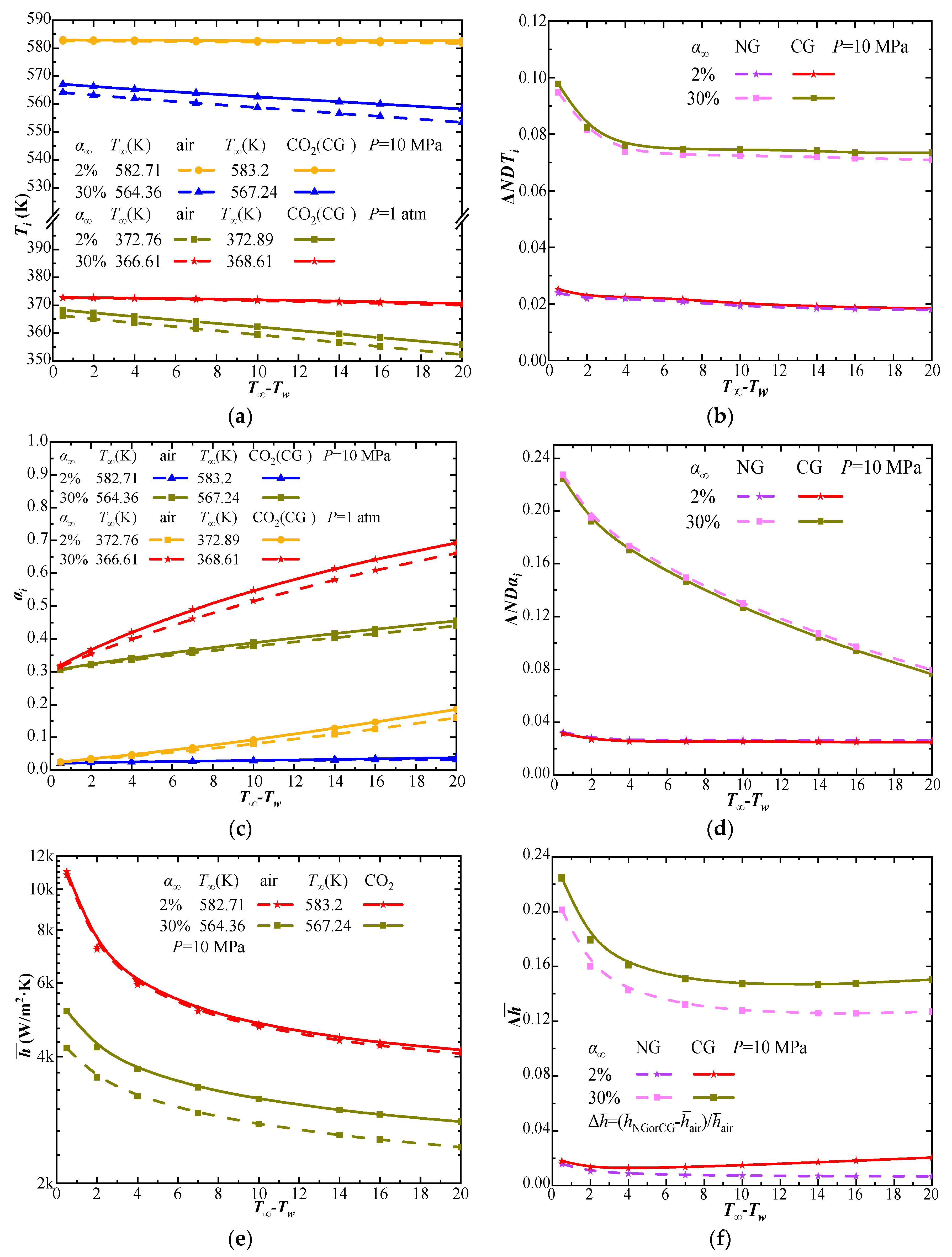
4.1. The Effect of CO₂ Solubility on Steam–CO₂ Mixture Condensation

The effect of CO₂ solubility on the condensation of the steam–CO₂ mixture is analyzed by comparing the simulation results of boundary layer models with and without considering CO₂ solubility, which have been marked as the CG model and the NG model, respectively. By taking the horizontal plate as an example, Figure 5 gives the average HTC and q/q₀ curves versus the subcooling. The inlet CO₂ mass percentages shown in Figure 5 are taken at 2%, 30%, and 80%, and the simulation results of CG and NG models are both given and compared under total pressure conditions of 1 atm, 1 MPa, and 10 MPa. Steam–CO₂ mixture condensation data curves calculated by CG (solid curve) and NG (dash curve) boundary layer models are different. Although the solid and dash curves are closer to each other at total pressure conditions of 1 atm and 1 MPa, they can be distinguished under 10 MPa conditions. All the distinguishable curves presented in Figure 5 show that the average HTC and q/q₀ curves calculated by the CG model are larger than those calculated by the NG model under the same conditions. Moreover, under 10 MPa, increases in the concentration and differences in the average HTC curve between the CG and NG models are found. This indicates that the solubility of CO₂ is an enhancement or reduction alleviation effect of the steam–CO₂ condensation heat transfer.

The effect of CO₂ solubility on steam–CO₂ mixture condensation is different under different conditions, partly because of the different CO₂ solubility itself, which increases with increasing CO₂ partial pressure and decreases with temperature. For the small calculation range of subcooling in this study (≤20 K), the solubility of CO₂ is mainly controlled by the total pressure and the CO₂ percentage. When the total pressure is 1 atm and 1 MPa, the solid and dash curves are almost coincident in Figure 5, especially for Figure 5a,b; this is because the solubility of CO₂ is small under this condition. Thus, it is reasonable to regard CO₂ as an NCG under low-pressure conditions. As the pressure increases, the partial pressure of CO₂ on the surface of the condensate also gradually increases. At a total pressure of 10 MPa, the CG and NG models show significantly different simulation results. By comparing the curves in Figure 5a,c,e, with an increase in the CO₂ concentration, the differences in the average HTC values of the CG and NG models become more significant under the same total pressure levels. When the concentration reaches 80%, a reduction in the condensate heat transfer is significant, and q/q₀ is not discussed here.

The effect of CO₂ solubility on mixture condensation will influence the average HTC data. Figure 6a shows the average HTC deviations between CG and NG models and Figure 6b shows CO₂ solubility values under a total pressure of 10 MPa, in which ΔHTC is:

$$\mathsf{\Delta }HTC=\frac{{\overline{h}}_{CG}-{\overline{h}}_{NG}}{{\overline{h}}_{CG}}$$

(25)

For the inlet condition of 2% CO₂, the CO₂ solubility is around 0.6508–1.6401 g/kg water, and ΔHTC is the range of 0.218–4.4%; meanwhile, for the inlet condition of 30% CO₂, the CO₂ solubility is around 10.8774–25.3173 g/kg water and ΔHTC is around 1.4–3.5%; and for the inlet condition of 80% CO₂, the CO₂ solubility is around 36.1272–39.6 g/kg water and ΔHTC is around 2.117–3.005%. It can be found that with the increase in subcooling, the growth rate of low α_∞ is faster. This is because the mixed gas with lower α_∞ has better condensation and heat transfer conditions, the condensation mass flux is larger, and ΔHTC may show a faster growth trend. In conclusion, when subcooling increases, the solubility of CO₂ reduces the reduction in condensation heat transfer more obviously. The contrast of ΔHTC and S shows an increase in the total pressure and CO₂ concentration, and the low solubility of CO₂ is not negligible.

Figure 7a,b show the average temperature (T_i) and average mass percentage (α_i) curves at the gas–liquid interface under total pressure conditions of 1 atm and 10 MPa. Figure 7c shows a variation in the condensate film thickness along the horizontal plate at a subcooling rate of 7 K. The solubility of CO₂ is larger under a total pressure condition of 10 MPa, and its influence on T_i and α_i is more obvious. Similarly, CO₂ solubility is larger for a 30% CO₂ inlet condition than a 2% inlet CO₂ at the inlet because of the larger partial pressure, so it also has an influence on T_i and α_i. Through Figure 7b, the α_i calculated by the CG model is smaller than that calculated by the NG model, which indicates that the mechanism of CO₂ can promote condensation in order to reduce the accumulation of CO₂ at the gas–liquid interface. In Figure 7c, the effect of CO₂ solubility on the accumulation of condensate film on the plate can also be seen, but it is not very remarkable. The thickness of the liquid film in the CG model is greater than that in the NG model.

Therefore, when the total pressure is higher than 1 MPa, it is wrong to regard CO₂ as an NCG. It is necessary to consider the solubility of CO₂ in order to estimate the heat transfer of steam–CO₂ mixture condensation under high-pressure conditions. CO₂ solubility has an enhanced effect on condensation.

4.2. Comparison of the Steam–CO₂ Mixture Condensation Features with Steam–Air

Figure 8 shows the variation in condensation parameters of steam–CO₂ (CG model) and steam–air condensation mixtures at 1 atm and 10 MPa on the surface of a 0.2 m long horizontal plate. The velocity of the mixture is 1 m/s, and the CO₂ and air mass percentages at the inlet mixture gas are taken as 2% and 30%. As shown in Figure 8a, for the same mass percentage and other conditions of steam–CO₂ and steam–air mixtures, there is a remarkable difference in their condensation heat transfer parameters, which is only caused by the different components of CO₂ and air. The gas–liquid interface temperature of steam–CO₂ mixture condensation is higher than that of a steam–air mixture. Figure 8c shows that the percentage of CO₂ at the gas–liquid interface is higher than that of air. Since the solubility of CO₂ is small, its effect on condensation can be negligible in low-pressure conditions. Moreover, 10 MPa is selected as the total pressure of this part for the following data comparison. Figure 8b uses ΔNDT_i (the deviation in non-dimensional T_i) to compare the ratio of thermal resistance in the gas phase of NG or CG with air at 10 MPa.

$$\begin{array}{l}\mathsf{\Delta }ND{T}_i=\frac{{(T_{\mathrm{air}}-T_{\mathrm{NG}/\mathrm{CG}})}_{\infty }-{(T_{\mathrm{NG}/\mathrm{CG}}-T_{\mathrm{air}})}_{\infty }}{T_{\infty }-T_w}\\ ={(\frac{T_{\infty }-T_i}{T_{\infty }-T_w})}_{\mathrm{air}}-{(\frac{T_{\infty }-T_i}{T_{\infty }-T_w})}_{\mathrm{NG}/\mathrm{CG}}\end{array}$$

(26)

The physical significance of the first term represents the proportion of the gas-phase thermal resistance of steam–air total thermal resistance, and the second term represents the proportion of the gas-phase thermal resistance of steam–CO₂ (CG model or NG model) in the total resistance. Both terms are dimensionless parameters. Due to the differences in physical properties, under the same condition in α_∞, the gas-phase thermal resistance of steam–air mixture condensation is greater than that of the steam–CO₂ mixture. Given the micro-soluble nature of CO₂, the gas-phase thermal resistance calculated by the CG model is lower than that calculated by the NG model, as shown in Figure 8a,b, due to the entry of CO₂ into the liquid phase. Figure 8d shows ΔNDα_i (the deviation in non-dimensional α_i), as given below:

$$\mathsf{\Delta }ND{\alpha }_i=\frac{{\alpha }_{i,\mathrm{air}}-{\alpha }_{i,\mathrm{NG}/\mathrm{CG}}}{{({\alpha }_i-{\alpha }_{\infty })}_{\mathrm{air}}}=1-\frac{{({\alpha }_i-{\alpha }_{\infty })}_{\mathrm{air}}}{{({\alpha }_i-{\alpha }_{\infty })}_{\mathrm{NG}/\mathrm{CG}}}$$

(27)

ΔNDα_i represents the CO₂ fraction difference at the steam–CO₂ and steam–air gas–liquid interface. In Figure 8d, the difference in ΔNDα_i increases with an increase in the CO₂ concentration and subcooling rate. Figure 8a–d indicate that the impact of CO₂ solubility at low pressures or concentrations is small, and the difference between mixture condensation is mainly reflected by the difference in the physical properties of air and CO₂. The physical parameters of the mixture gas considered in the boundary layer model are viscosity, thermal conductivity, specific heat capacity, density, and the diffusion coefficient. Moreover, the low solubility of CO₂ at high pressures and concentrations is one of the most influential physical properties.

The results in Figure 8 show that different gas components also have a significant effect on the condensation features, which can explain why some existing correlations cannot be used to predict the condensation of steam–CO₂ [27]. Figure 8e,f show the $\overline{h}$ and Δ$\overline{h}$ of the mixtures of steam–CO₂ (both the NG model and the CG model) and steam–air on the horizontal plate surface. The heat transfer coefficient of the steam–CO₂ mixture is higher than that of the steam–air mixture. Moreover, the difference in the average HTC becomes more obvious with an increase in the subcooling and concentration of CO₂ or air; when the subcooling is 20 K and α_∞ is 30%, the Δ$\overline{h}$ reaches 16%.

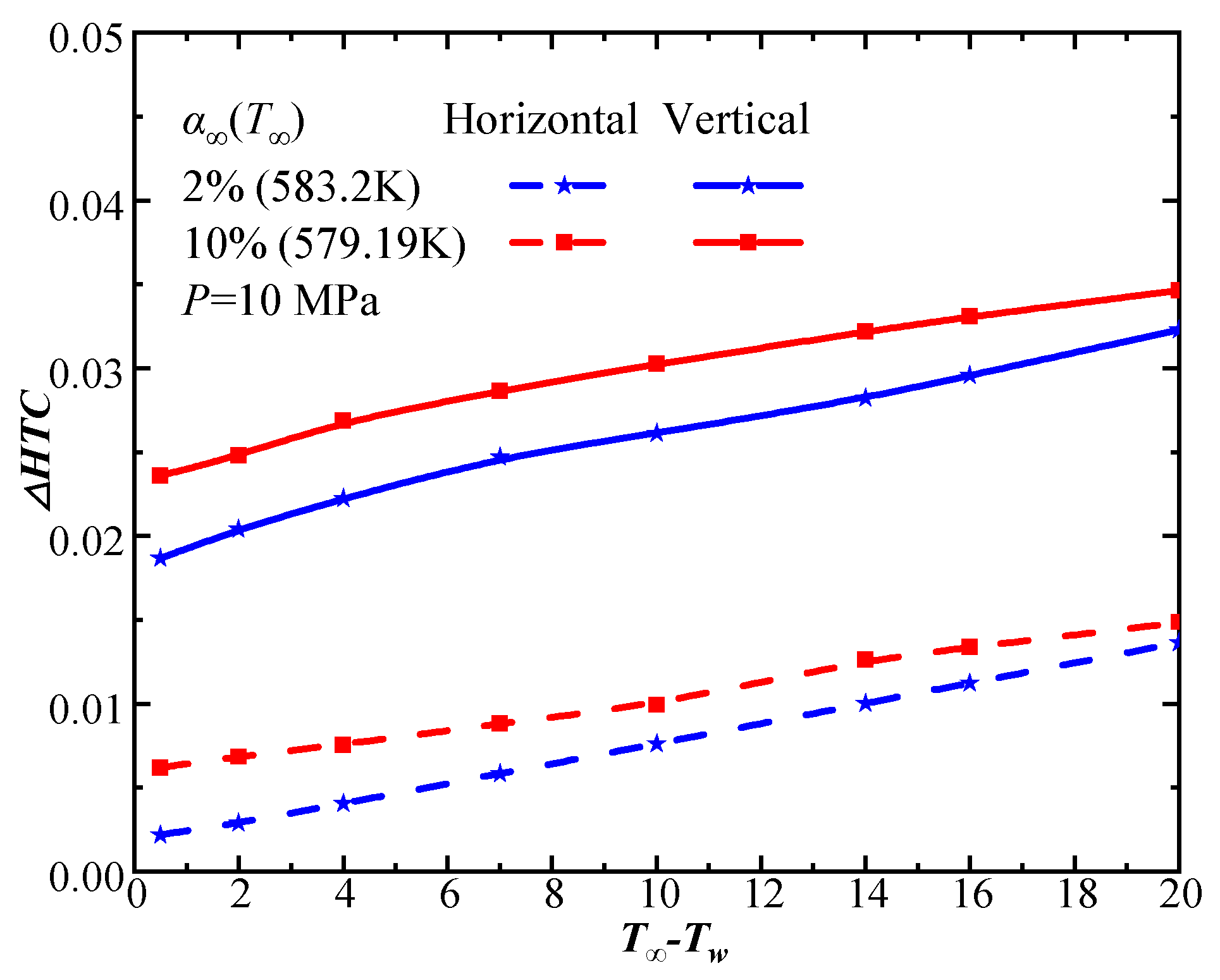
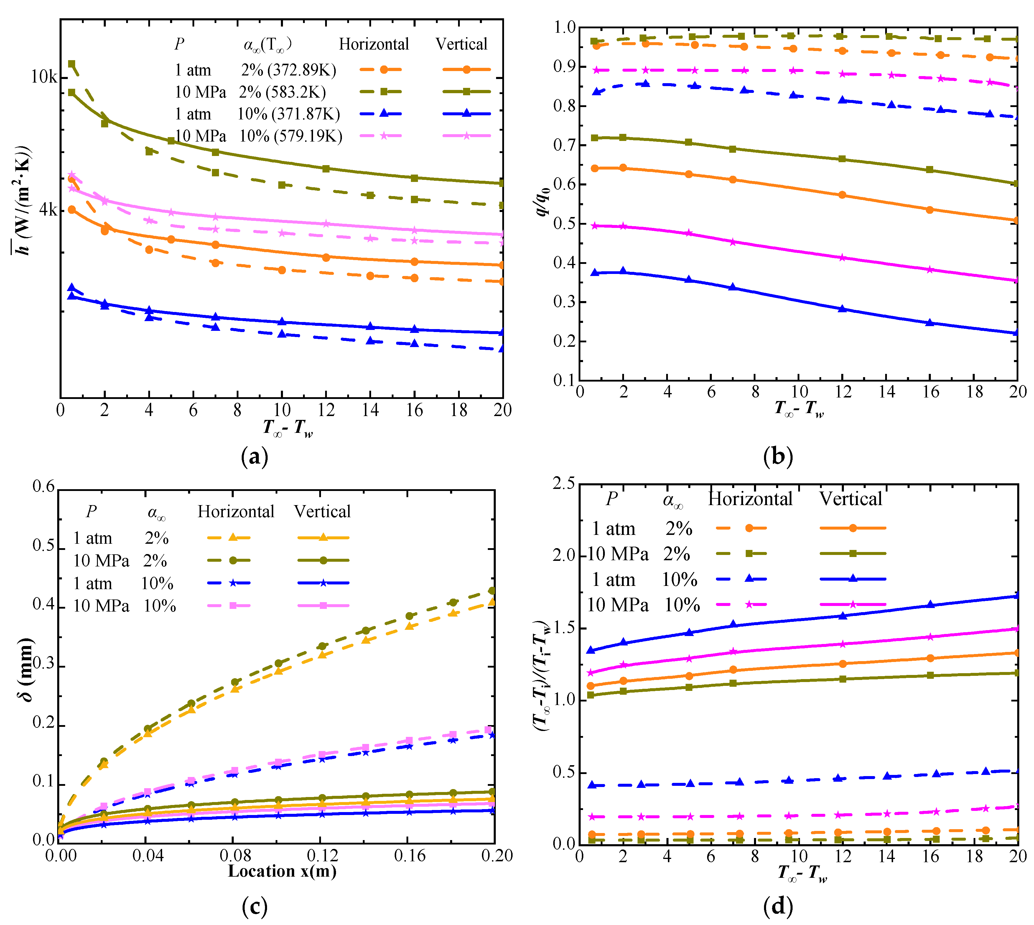
4.3. Comparison of Steam–CO₂ Mixture Condensation Features on Horizontal and Vertical Plates

Due to the different inlet velocity settings and driving forces of the liquid film, the boundary layer models of the steam–CO₂ mixture condensation on the surfaces of the vertical and horizontal plates are not the same.

Figure 9 shows a comparison of the condensation ΔHTC values at CO₂ inlet fractions of 2% and 10% on horizontal and vertical plates at 10 MPa. The result shows that the ΔHTC caused by the solubility of CO₂ on a vertical plate is larger than that on a horizontal plate under the same α_∞. Thus, the effect of CO₂ solubility on improvements in average HTC values on the vertical plate is larger than those on the horizontal plate. On the vertical plate, the gas phase accounts for the main thermal resistance. However, it becomes smaller when CO₂ dissolves in the liquid phase.

Figure 10 shows a comparison of some other calculation results on the condensation on horizontal and vertical plate surfaces. Figure 10a shows the calculation results of the average HTC values at the inlet CO₂ mass fractions of 2% and 10% under total pressure conditions of 1 atm and 10 MPa. The average HTC condensation value on the vertical plate is higher than that on the horizontal plate under a very small subcooling regime. This shows the advantages of using gravity to drain the condensate compared with using gas flow.

Figure 10b shows the heat transfer reduction (q/q₀) curves of the steam–CO₂ mixture condensation, and the label is same as Figure 10a. Condensation on the horizontal plate surface is significantly less affected by CO₂ than that on the vertical surface at the same CO₂ mass fraction. Due to the influence of gravity, the thickness of the liquid film accumulated in the horizontal plate is thicker than the vertical plate, which can be confirmed by the calculation of the thickness of the local liquid film in Figure 10c. With an increase in the CO₂ mass fraction, the condensation heat transfer is reduced and the accumulation of liquid film decreases, so the thickness of the liquid film becomes thinner for larger α_∞ conditions in Figure 10c. In addition, with the increase in pressure, an improvement is shown in the reduction in condensation heat transfer, and the condensate quality also increases.

Through the above analysis, at medium and low concentrations, the concentration of condensate is the main factor determining the thermal resistance to condensation on the horizontal plate. As shown in Figure 10c, compared with the vertical plate, the heat transfer reduction in the horizontal plate is not sensitive to changes in CO₂ concentration. As the thickness of the liquid film covered by the vertical plate is thinner, the thermal resistance in the liquid phase is smaller than that in the gas phase. Figure 10d shows the ratio of the temperature difference in the gas boundary layer and the liquid film, which represents the relative thermal resistance of both the gas phase and the liquid phase. Figure 10d shows that the thermal resistance in the gas phase is higher than that in the liquid phase on the vertical plate. Thus, a small mass fraction of CO₂ will have a significant impact.

5. Conclusions

We carried out the theoretical modeling and simulation of the boundary layer for the condensation of the steam–CO₂ mixture on the surface of horizontal and vertical plates. (i) Based on the boundary layer theory, CO₂ is regarded as an NCG, and the solubility of CO₂ also matters. The boundary layer model is modified to obtain a new CG model. At the same time, a new iterative calculation method is used in the iterative calculation to extend the calculation range of the NG model, including extending the NG model to calculate the steam–air mixed condensation to calculate the steam–CO₂ mixed condensation and expanding the calculation range of α_∞ and pressure. (ii) The influence of CO₂ solubility on the heat transfer of mixed gas condensation is clarified, which adds a consideration factor for the next research study on steam–CO₂ condensation heat transfer. Comparing the differences between steam–CO₂ and steam–air, besides the difference in gas physical properties, solubility was also the factor that caused these differences. (iii) The effect of CO₂ solubility on the condensation heat transfer of mixed gas on the horizontal plate and vertical plate was compared. The main conclusions are as follows:

Due to the slight solubility of CO₂, part of CO₂ can pass through the gas–liquid interface and enter the liquid film, and the CO₂ accumulation at the surface of the liquid film decreases, which reduces the condensation heat transfer. However, this effect is only manifested under high-pressure conditions, where the solubility of CO₂ is non-negligible. In this paper, the data show that when the total pressure of the steam–CO₂ mixture is higher than 1 MPa, the influence of the slightly soluble CO₂ on the condensation of the mixed gas should be considered.

The same mass fraction condition was selected to compare the condensation features with different mixture gases. The differences in condensation heat transfer of steam–CO₂ and steam–air mixtures under the same conditions are caused by different physical properties of different components at low pressures and low concentrations. CO₂ reduces condensation less compared to air. When the total pressure or concentration is high, the slight solubility of CO₂ can also be regarded as a physical property, which has an effect on condensation heat transfer.

Within the calculation range, the effect of the CO₂ concentration on the condensation of the horizontal plate surface is smaller than that of the vertical plate surface. However, the effect of CO₂ solubility in terms of improvements in the heat transfer coefficient of the vertical plate is better than that of the horizontal plate.

For the NG and CG models of the developed boundary layer theory, the inclination angle β of the plate was introduced to unify one set of models of the horizontal plate and vertical plate to determine the influence of geometric position on condensation heat transfer. Based on the limitations of the model, CFD was used in the following calculation to simulate a new scheme containing a high mass fraction of CO₂ in steam–CO₂ condensation, and the influence of solubility was further compared. The rationality of simulation calculation is to show the difference between the two calculation schemes.

References

1. Mualim, A.; Huda, H.; Altway, A.; Sutikno, J.P.; Handogo, P. Evaluation of multiple time carbon capture and storage network with capital-carbon trade-off. J. Clean. Prod. 2021, 291, 125710. [Google Scholar] [CrossRef]
2. Freire, A.L.; Jose, H.J.; Moreira, R.F.P.M. Potential applications for geopolymers in carbon capture and storage. Int. J. Greenh. Gas Control. 2022, 118, 103687. [Google Scholar] [CrossRef]
3. Intergovernmental Panel on Climate Change (IPCC). Contribution of Working Group I. Contribution to the Sixth Assessment Report, the Physical Science Basis; Cambridge University Press: Cambridge, UK, 2021. [Google Scholar]
4. Chen, Y.P.; Zhu, Z.L.; Wu, J.F.; Yang, S.F.; Zhang, B.H. A novel LNG/CO2 combustion gas and steam mixture cycle with energy storage and CO2 capture. Energy 2017, 120, 128–137. [Google Scholar] [CrossRef]
5. Zhao, W.J.; Chen, Y.P.; Wu, J.F.; Zhu, Z.L.; Wang, J. Study on CO2 capture upgrading of existing coal fired power plants with gas-H2O mixture cycle and supercritical water coal gasification. Int. J. Greenh. Gas Control. 2021, 112, 103482. [Google Scholar] [CrossRef]
6. High, M.; Patzschke, C.F.; Zheng, L.Y.; Zeng, D.W.; Gavalda-Diaz, O.; Ding, N.; Chien, K.H.H.; Zhang, Z.L.; Wilson, G.E.; Berenov, A.V.; et al. Precursor engineering of hydrotalcite-derived redox sorbents for reversible and stable thermochemical oxygen storage. Nat. Commun. 2022, 13, 5109. [Google Scholar] [CrossRef]
7. Yi, Q.J.; Tian, M.C.; Yan, W.J.; Qu, X.H.; Chen, X.B. Visualization study of the influence of non-condensable gas on steam condensation heat transfer. Appl. Therm. Eng. 2016, 106, 13–21. [Google Scholar] [CrossRef]
8. Kuhn, S.Z.; Schrock, V.E.; Peterson, P.F. An investigation of condensation from steam-gas mixtures flowing downward inside a vertical tube. Nucl. Eng. Des. 1997, 177, 53–69. [Google Scholar] [CrossRef]
9. Rose, J.W. Approximate equations for forced-convection condensation in the presence of a non-condensing gas on a flat-plate and horizontal tube. Int. J. Heat Mass Transf. 1980, 23, 539–546. [Google Scholar] [CrossRef]
10. Huhtiniemi, I.K.; Corradini, M.L. Condensation in the presence of noncondensable gases. Nucl. Eng. Des. 1993, 141, 429–446. [Google Scholar] [CrossRef]
11. Kang, H.C.; Kim, M.H. Characteristics of film condensation of supersaturated steam-air mixture on a flat plate. Int. J. Multiph. Flow 1999, 25, 1601–1618. [Google Scholar] [CrossRef]
12. Aldiwany, H.K.; Rose, J.W. Free convection film condensation of steam in the presence of non-condensing gases. Int. J. Heat Mass Transf. 1973, 16, 1359–1369. [Google Scholar] [CrossRef]
13. Morrison, J.N.A.; Deans, J. Augmentation of steam condensation heat transfer by addition of ammonia. Int. J. Heat Mass Transf. 1997, 40, 765–772. [Google Scholar] [CrossRef]
14. Sparrow, E.M.; Yang, J.W.; Scott, C.J. Free convection in an air-water vapor boundary layer. Int. J. Heat Mass Transf. 1966, 9, 53. [Google Scholar] [CrossRef]
15. Sparrow, E.M.; Minkowycz, W.J.; Saddy, M. Forced convection condensation in the presence of noncondensables and interfacial resistance. Int. J. Heat Mass Transf. 1967, 10, 1829–1845. [Google Scholar] [CrossRef]
16. Minkowycz, W.J.; Sparrow, E.M. Condensation heat transfer in the presence of noncondensables, interfacial resistance, superheating, variable properties, and diffusion. Int. J. Heat Mass Transf. 1966, 9, 1125–1144. [Google Scholar] [CrossRef]
17. Millsaps, K.; Pohlhausen, K. The Laminar-free-convective-heat transfer from the outer surface of a vertical circular cylinder. J. Aeronaut. Sci. 1958, 25, 357–360. [Google Scholar] [CrossRef]
18. Popiel, C.O. Free convection heat transfer from vertical slender cylinders: A review. Heat Transf. Eng. 2008, 29, 521–536. [Google Scholar] [CrossRef]
19. Angelino, M.; Boghi, A.; Gori, F. Numerical solution of three-dimensional rectangular submerged jets with the evidence of the undisturbed region of flow. Numer. Heat Transf. Part A 2016, 70, 815–830. [Google Scholar] [CrossRef]
20. Boghi, A.; Venuta, I.D.; Gori, F. Passive scalar diffusion in the near field region of turbulent rectangular submerged free jets. Int. J. Heat Mass Transf. 2017, 112, 1017–1031. [Google Scholar] [CrossRef]
21. Boghi, A.; Angelino, M.; Gori, F. Numerical Evidence of an Undisturbed Region of Flow in Turbulent Rectangular Submerged Free Jet. Numer. Heat Transf. 2016, 70, 14–29. [Google Scholar] [CrossRef]
22. Hossein, S.; Nima, A.; Ali, J. Effects of Applying Brand-New Designs on the Performance of PEM Fuel Cell and Water Flooding Phenomena. Iran. J. Chem. Chem. Eng.-Int. Engl. Ed. 2022, 41, 618–635. [Google Scholar]
23. Dehbi, A.; Janasza, F.; Bell, B. Prediction of steam condensation in the presence of noncondensable gases using a CFD-based approach. Nucl. Eng. Des. 2013, 258, 199–210. [Google Scholar] [CrossRef]
24. Li, J.-D. CFD simulation of water vapor condensation in the presence of non-condensable gas in vertical cylindrical condensers. Int. J. Heat Mass Transf. 2013, 57, 708–721. [Google Scholar] [CrossRef] [PubMed]
25. Choudhury, R.; Das, U.J. Viscoelastic effects on the three- Dimensional hydrodynamic flow past a vertical porous plate. Int. J. Heat Technol. Assoc. 2013, 31, 1–8. [Google Scholar]
26. Ge, M.H.; Zhao, J.; Wang, S.X. Experimental investigation of steam condensation with high concentration CO2 on a horizontal tube. Appl. Therm. Eng. 2013, 61, 334–343. [Google Scholar] [CrossRef]
27. Ge, M.H.; Wang, S.X.; Zhao, J.; Zhao, Y.L.; Liu, L.S. Condensation of steam with high CO2 concentration on a vertical plate. Exp. Therm. Fluid Sci. 2016, 75, 147–155. [Google Scholar] [CrossRef]
28. Lu, J.H.; Cao, H.S.; Li, J.M. Experimental study of condensation heat transfer of steam in the presence of non-condensable gas CO2 on a horizontal tube at sub-atmospheric pressure. Exp. Therm. Fluid Sci. 2019, 105, 278–288. [Google Scholar] [CrossRef]
29. Takami, K.M.; Mahmoudi, J.; Time, R.W. A simulated H2O/CO2 condenser design for oxy-fuel CO2 capture process. Energy Procedia 2009, 1, 1443–1450. [Google Scholar] [CrossRef]
30. Lu, J.H.; Ren, K.X.; Tang, J.J. Numerical simulations of laminar film condensation of H2O/Air or H2O/CO2 on a vertical plate. Heat Transf. Eng. 2022, 44, 720–733. [Google Scholar] [CrossRef]
31. Han, J.M.; Shin, H.Y.; Min, B.M. Measurement and correlation of high pressure phase behavior of carbon dioxide+water system. Ind. Eng. Chem. Eng. Data 2009, 15, 212–216. [Google Scholar] [CrossRef]
32. Lucile, F.; Cezac, P.; Contamine, F.; Serin, J.P.; Houssin, D.; Arpentinier, P. Solubility of Carbon Dioxide in Water and Aqueous Solution Containing Sodium Hydroxide at Temperatures from (293.15 to 393.15) K and Pressure up to 5 MPa: Experimental Measurements. J. Chem. Eng. Data 2012, 57, 784–789. [Google Scholar] [CrossRef]
33. Hou, S.X.; Maitland, G.C.; Trusler, J.P.M. Measurement and modeling of the phase behavior of the (carbon dioxide+water) mixture at temperature from 298.15 K to 448.15 K. J. Supercrit. Fluids 2013, 73, 87–96. [Google Scholar] [CrossRef]
34. Meyer, C.W.; Harvey, A.H. Dew-point measurements for water in compressed carbon dioxide. AICHE J. 2015, 61, 2913–2925. [Google Scholar] [CrossRef]
35. Mao, S.D.; Zhang, D.H.; Li, Y.Q.; Liu, N.Q. An improved model for calculating CO2 solubility in aqueous NaCl solutions and the application to CO2-H2O-NaCl fluid inclusions. Chem. Geol. 2013, 347, 43–58. [Google Scholar] [CrossRef]
36. Liu, G.Q.; Ma, L.X. Chemical Physics Data; Chemical Industry Press: Beijing, China, 2002; pp. 84–85. [Google Scholar]
37. Duan, Z.H.; Sun, R.; Zhu, C.; Chou, I.M. An improved model for the calculation of CO2 solubility in aqueous solutions containing Na+, K+, Ca2+, Mg2+, Cl, SO42−. Mar. Chem. 2006, 98, 131–139. [Google Scholar] [CrossRef]
38. Valtz, A.; Chapoy, A.; Coquelet, C.; Paricaud, P.; Richon, D. Vapor-liquid equilibria in the carbon dioxide–water system, measurement and modelling from 278.2 to 318.2 K. Fluid Phase Equilibria 2004, 226, 333–344. [Google Scholar] [CrossRef]
39. Fronk, B.M.; Garimella, S. Condensation of ammonia and high-temperature-glide zeotropic ammonia/water mixtures in minichannels-Part II: Heat transfer models. Int. J. Heat Mass Transf. 2016, 101, 1357–1373. [Google Scholar] [CrossRef]
40. Wang, X.Y.; Ming, Z.Y. Measurements of gas enthalpy of dissolution. China Acad. J. Electron. Publ. House 1987, 1, 62–64. [Google Scholar]
41. Koschel, D.; Coxam, J.Y.; Rodier, L.; Majer, V. Enthalpy and solubility data of CO2 in water and NaCl(aq) at conditions of interest for geological sequestration. Fluid Phase Equilibria 2006, 247, 107–120. [Google Scholar] [CrossRef]
42. NIST. NIST Reference Fluid Thermodynamic and Transport Properties-REFPROP (Version 9.1); NIST Stand Ref Database 2007:23; National Institute of Standards and Technology: Gaithersburg, MD, USA, 2013.
43. Othmer, D.F. The condensation of steam. Ind. Eng. Chem. 1929, 21, 576–583. [Google Scholar] [CrossRef]
Figure 1. Schematic diagram of a boundary layer model of steam–CO2 mixture condensation.
Applsci 13 05747 g001
Figure 2. Iterative for Tix and αix.
Applsci 13 05747 g002
Figure 3. Comparison between the boundary layer model data and data from Ge et al. [27] study (P = 101.325 kPa, α = 34.3%, T = 367.74 K).
Applsci 13 05747 g003
Figure 4. Data trends of steam–CO2 condensation on the flat plate. (a) Variation in hx along the horizontal plate; (b) Variation in δ along the horizontal plate; (c) Condensation film thickness and gas–liquid interface velocity along the vertical plate.
Applsci 13 05747 g004
Figure 5. Comparison of CG and NG models for steam–CO2 mixture condensation (U = 1 m/s; L = 0.2 m). (a) α=2% average HTC; (b) α=2% q/q0; (c) α=30% average HTC; (d) α=30% q/q0; (e) α=80% average HTC.
Applsci 13 05747 g005
Figure 6. Comparison of ΔHTC and CO2 solubility values at CO2 inlet fractions of 2%, 30%, and 80% (U = 1 m/s; L = 0.2 m). (a) Comparison of ΔHTC at different α; (b) Comparison of S at different α.
Applsci 13 05747 g006
Figure 7. Comparison of Ti, αi, and δ curves at total pressures of 10 MPa. (a) Ti versus subcooling; (b) αi versus subcooling; (c) Film thickness along the horizontal plate at 7 K subcooling (U = 1 m/s; L = 0.2 m).
Applsci 13 05747 g007
Figure 8. Comparison of steam–CO2 and steam–air mixture condensation on horizontal plate at the same inlet CO2 and air mass percentage (U = 1 m/s; L = 0.2 m). (a) Variation in Ti with subcooling; (b) Variation in ΔNDTi with subcooling; (c) Variation in αi with subcooling; (d) Variation in ΔNDαi with subcooling; (e) Variation in h ¯ with subcooling; (f) Variation in Δ h ¯ with subcooling.
Applsci 13 05747 g008
Figure 9. Comparison of condensation ΔHTC at CO2 inlet fractions of 2% and 10% on horizontal and vertical plates (U = 1 m/s; L = 0.2 m).
Applsci 13 05747 g009
Figure 10. Comparison of steam–CO2 mixture condensation on the horizontal and vertical surfaces. (a) Average HTC; (b) q/q0; (c) δ; (d) Ratio of temperature differences in gas and liquid-phases.
Applsci 13 05747 g010