Abstract
Bike sharing systems have become a sustainable alternative to motorized private transport in urban areas. However, users often face high costs and availability issues due to the operational effort required to redistribute bicycles between stations. For addressing those issues, the AuRa (Autonomes Rad, Eng. Autonomous Bicycle) project introduces a new mobility offer in terms of an on-demand, shared-use, self-driving cargo bikes service (OSABS) that enables automated redistribution. Within the project, we develop different order management and rebalancing strategies and validate them using simulation models. One prerequisite for this is sound demand scenarios. However, due to the novelty of OSABS, there is currently no information about its utilization. Consequently, the objective of this study was to develop an approach for defining OSABS demand scenarios in a temporally and spatially disaggregated manner as an input for simulation models. Therefore, we first derived city-wide usage potentials of OSABS from a survey on mobility needs. We then spatially and temporally disaggregated the determined usage likelihood using travel demand matrices and usage patterns from a conventional bike-sharing system, respectively. Finally, we performed cluster analyses on the resulting annual demand to summarize sections of the yearly profile into representative units and thus reduce the simulation effort. As we applied this approach as a case study to the city of Magdeburg, Germany, we could show that our methodology enables the determination of reasonable OSABS demand scenarios from scratch. Furthermore, we were able to show that annual usage patterns of (conventional) bike sharing systems can be modeled by using demand data for only eight representative weeks.
1. Introduction
As a consequence of the persistent trend towards urbanization [1], cities suffer from negative externalities (traffic congestion, air pollution, noise, etc.) caused by the increase in urban mobility [2,3,4,5]. Since motorized individual transport comprises a sizable proportion of those negative effects, policymakers consider the promotion of active mobility (i.e., walking and cycling) as a way to address the key challenges of growing urban transport [6]. In this regard, bike sharing systems have gained popularity, as they provide a sustainable and affordable alternative to motorized vehicles. Therefore, these systems are increasingly implemented in cities around the world [7].
However, as pointed out by previous studies (e.g., Refs. [8,9,10,11]), bike sharing systems commonly face spatial and temporal fluctuations in bike rentals, which lead to uneven distribution of bicycles among stations and thus to unavailability and customer dissatisfaction. To prevent supply imbalance, system operators have to deploy costly and unsustainable redistribution operations, which are usually performed by trucks or trailers [8]. Further, although bike sharing systems are highly integrated into public transport, they do not provide door-to-door mobility, since users still need to walk to a certain bike sharing station and often cannot return the bike at their final destination [12].
Zug et al. [13] provided an approach to address the associated ecological and economic disadvantages by introducing a framework for the utilization of shared autonomous bicycles in the context of mobility as a service concept. Within the AuRa (Autonomes Rad, Eng. autonomous bike) research project, we are currently further enhancing this approach as we aim to develop an on-demand, shared-use, self-driving cargo bikes service (OSABS). Through leveraging autonomous driving functions, the system enables automated demand-responsive rebalancing and thus reduces rebalancing effort and service unavailability. In addition, the system enables door-to-door mobility through reserved on-demand provision, with the possibility of transporting cargo and economically viable applications in less dense urban areas [13].
As outlined in [14], we therefore believe that OSABS, by offering efficient, accessible, and eco-friendly transportation alternatives, not only addresses the shortcomings of conventional bike sharing systems but also significantly contributes to creating more livable urban environments. Through a reduction in motorized traffic, OSABS leads to a multitude of benefits, including increased traffic safety, the redistribution of public spaces, and a reduction in negative environmental impacts. Further, the system’s versatility and user-centric design, as indicated by the high acceptance and usage intentions reported in [15], suggest its potential to replace not only conventional bike sharing but also other short-distance transportation modes, including walking, biking, and public transport.
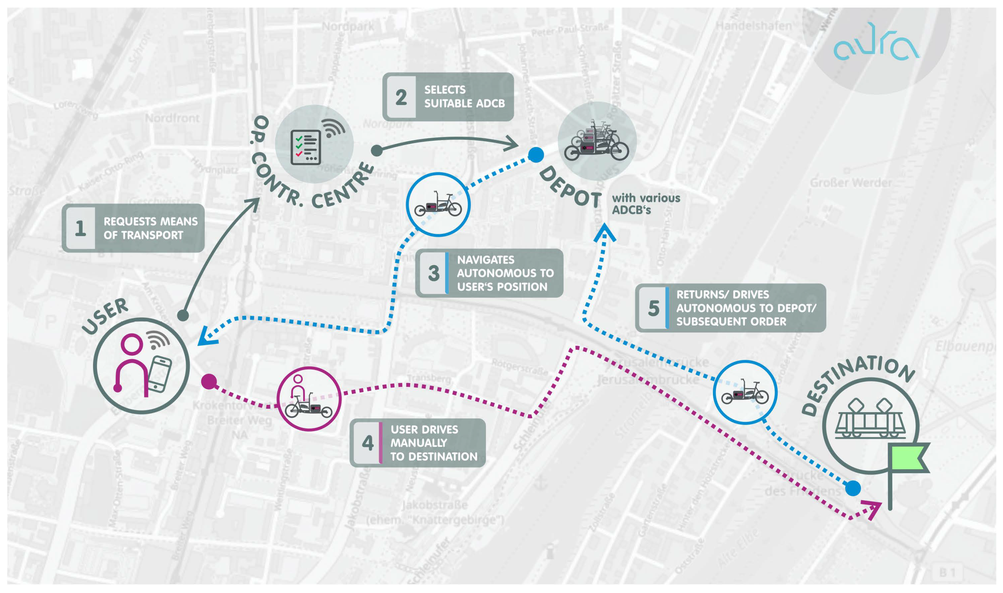
Figure 1 shows the conceptual OSABS workflow. Initially, the user requests an autonomous driving cargo bike (ADCB) via a smartphone app. As a next step, the Operation Control Center (OCC) selects a suitable bike which will then autonomously drive to the user’s location. After the bike arrives, the user manually rides it to a desired location. At the destination, the user releases the bike and it autonomously drives to the next customer or to a waiting or charging station (e.g., Refs. [16,17,18]).
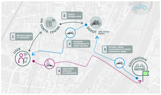
Figure 1.
OSABS workflow.
In order to explore its potential for sustainable urban mobility and provide a better understanding of the novel system, we evaluate different strategies (order management, station distribution, and rebalancing) and energy supply technologies using an agent-based simulation model [17,18]. Next to various business cases, demand scenarios that predict the hourly use of OSABS for a one-year period are a key input for the simulation model. However, due to the novelty of OSABS, there is currently no information about its utilization. Within this paper, we therefore provide a data-driven approach that aims at modeling different demand scenarios for OSABS in a temporally and spatially disaggregated manner.
Our contributions are three-fold. First, we identify the usage potentials of OSABS as a replacement for conventional modes of transport. Second, by analyzing and clustering trip data from a conventional bike sharing system in Hamburg, Germany, we show that annual usage patterns can be modeled with trip data for only eight representational weeks. Finally, we propose a methodology that enables traffic prediction for novel transportation systems such as OSABS with high temporal and spatial granularity by using traffic demand models and historical bike sharing data. We illustrate this approach by applying it as a case study to the city of Magdeburg, Germany. As our results show, the proposed approach provides reasonable predictions of hourly OSABS demand. Additionally, since we enable the representation of annual patterns with only eight weeks, we can reduce the computational effort of simulating annual OSABS usage by nearly 85%.
The remainder of this paper is organized as follows. Within the next two sections, we review a collection of related publications on different aspects of bike sharing and demand prediction (Section 2) and outline the OSABS simulation model (Section 3). In Section 4, we then describe our demand generation methodology and its application as a case study. In Section 5, we present our modeling results. Finally, in Section 6, we discuss our findings, summarize our work, and highlight future research initiatives.
2. Literature Review
Due to the steady growth of conventional bike sharing systems worldwide in the past decades [7], these systems have been subject to increasing research interest. In the recent literature, a variety of methods and approaches have been used to access different aspects of bike sharing. The three categories related to the aim of our work are demand prediction, system design, and influencing factors.
2.1. Prediction of Bike Sharing Demand
Based on their spatial granularity, the existing methods and approaches of predicting bike sharing demand can be classified into three groups: system-level prediction, cluster-level prediction, and station-level prediction [19].
For system-level prediction, Borgnat et al. [20] analyzed a public bike sharing scheme in Lyon, France, using a combination of statistical signal processing tools to derive temporal usage patterns for a typical week. While including internal (subscribers, number of available bikes) and external (temperature and precipitation) factors, those tools were also used to estimate the number of rentals within the next hour.
Additional research on predicting bike sharing demand at the system level was proposed by Giot and Cherrier [21]. They applied different regression models to predict the hourly bike sharing usage up to 24 h ahead. The used regressors (weather, previous bike usage, and holiday) were obtained from a public dataset containing two years of information on the Washington DC bike sharing system. Within their study, Ridge Regression and AdaBoost Regression were shown to have the best performance.
An approach for system-wide usage prediction over a longer time period was proposed by Cantelmo et al. [22]. Within their study, they introduced a clustering technique for synthesizing mobility data in order to obtain recursive mobility patterns. By validating their approach with existing data from New York City, Cantelmo et al. could show that combining those patterns with weather data enables the accurate prediction of daily bike sharing demand [22].
However, concerning the objective of our study, the presented methods cannot be applied to OSABS demand generation, since the usage can be predicted either for only a few hours ahead [20,21] or with insufficient temporal granularity [22]. An additional impediment to transferability emerges from the constraint that employing data derived from already implemented conventional bike sharing systems only allows for the prediction of demand within these particular systems. This also applies to the multitude of cluster-based (e.g., Refs. [9,11,23,24]) or station-based (e.g., Refs. [8,19,25,26,27,28,29,30,31,32,33]) approaches, as they rely on already existing stations (or subsets of stations).
2.2. Bike Sharing System Design
To estimate potential bike sharing demand in cities or countries where such systems have not yet been implemented, Todd et al. [34] analyzed data from 322 bike sharing schemes and divided them into five main groups, which were further classified into subgroups with regard to usage, contextual indicators, and the behavioral characteristics of their users. According to their study, this enables a global comparison of scheme performance and provides a basis for new schemes to recognize existing BSS with comparable characteristics that can serve as a reference for predicting potential user demand. However, this approach only allows for a rough estimation of demand on a system level while lacking spatial granularity.
Further, Frade and Ribeiro [35] proposed a methodology to relate bike sharing demand with external characteristics that affect bicycle use. These are trip distance and purpose, slope inclination, and the presence of bike lanes. Within their study, the definition of demand is accomplished in two steps: quantifying demand based on other case studies and defining the effect on demand caused by trip and physical city characteristics. However, we are not able to apply this approach to OSABS demand generation since, due to the novelty of OSABS, it was not possible to determine demand based on case studies from existing systems.
Another approach on the dimensioning of bike sharing systems was presented by Garcia-Gutierrez et al. [36]. To enable the prediction of potential bike sharing usage, they derived mobility patterns from a large-scale mobility survey in Mexico. Further, they generated utility models for different modes of transport (foot, bike, public transport, car) based on declared preferences surveys. In combination with mobility patterns, those utility functions enabled the determination of initial bicycle travel matrices. But, since we aim to complement all conventional modes of transport (including bicycles) with OSABS, this approach is also not feasible for us.
2.3. Factors Influencing Bike Sharing Utilization
According to Chen et al. [37], bike sharing usage patterns are mainly impacted by two types of contextual factors. Those include common contextual factors that occur frequently and affect the whole system (e.g., weather and time-related variables). In addition, there are opportunistic contextual factors which happen irregularly and affect only a subset of the system (e.g., social and traffic events). While some studies investigate the effects of opportunistic contextual factors (e.g., calendar events [38] or transit disruption [39]), common contextual factors are more frequently the subject of the recent literature.
To identify temporal usage patterns, Koska et al. [40] analyzed trip data from five German bike sharing schemes. Their findings show that during weekdays bike sharing demand has a slight morning peak and a larger peak in the afternoon. Similar results were obtained by Miranda-Moreno and Nosal [41] during their analysis of a bike sharing system in Montreal, Canada.
On a larger scale, O’Brien et al. [42] analyzed 38 global bike sharing systems and classified them based on temporal characteristics and associated user types. A large proportion of the considered systems also showed two weekday peaks (morning and afternoon) and a broad afternoon peak at weekends, with predicted user types being commuters and weekend leisure users. However, O’Brien et al. also identified further systems that, for example, are primarily used on weekends (leisure users) or have more than two commuter peaks per day (commuters with some utility users) [42]. The temporal characteristics of an even larger number of 322 global bike sharing schemes can also be obtained from Todd et al. [34].
Gebhart and Noland [43] analyzed the effect of different weather variables on bike sharing trips in Washington, DC, USA. Consistent with other studies (e.g., Refs. [38,44,45,46]), their results found that adverse weather like cold temperatures, rain, and increased wind speeds decreases the number of bike sharing trips. In addition, Caulfield et al. [47] claimed that not only the number of trips but also the travel time increase during good weather conditions. In contrast, several studies suggest that temperature has a negative impact on bike sharing demand when it exceeds a certain level [8,10,48].
While looking at temporal and weather effects, An et al. [44] additionally considered natural and built environments influencing bike sharing trips in New York City, USA. However, their findings show that weather impacts bike trips more than topography, infrastructure, or land use mix.
Furthermore, in correlation with previously presented effects of weather variables, several studies could show that the yearly trend in bike sharing usage can be classified into three periods. This includes an off season with low demand during winter months, a main season with high demand during summer months, and a transition phase with growing or falling demand in spring and fall months, respectively [28,40]. This indicates that the long-term influence of weather variables on bike sharing usage behavior can be also expressed through temporal patterns (in terms of yearly profiles or seasons).
In addition to weather conditions and time-related variables, there are many studies analyzing several other factors affecting bike sharing usage on a higher spatial granularity, such as sociodemographic and built environment characteristics (e.g., Refs. [45,49,50,51,52,53]). However, those factors predominantly impact usage behavior on a station level rather than on a system level. In addition, analyzing them requires specific data which are mostly valid for the considered study area only and thus limit the broad and easy transferability of our approach. Hence, related publications are beyond the scope of this work and will not be discussed any further.
For additional research in this regard, we recommend the work of Eren and Uz [54], Zhu et al. [55], and Guo et al. [56], who provide a comprehensive literature review of bike sharing influencing factors such as built environment and land use, public transportation, sociodemographic attributes, and safety. Another extensive overview of factors influencing micromobility sharing in general, classified into temporal, spatial, and weather-related factors, system-related factors, and user-related factors, is provided by Elmashhara et al. [57].
2.4. Implications from the Existing Literature
Based on the literature review, it becomes evident that existing approaches for determining bike sharing demand are not or only partly applicable to OSABS. In addition, a majority of the analyses of influencing factors considered in the literature involve significant amounts of location-specific data (e.g., built environment, public transportation, sociodemographic attributes, etc.) or affect the system on a short-term basis only (e.g., traffic or social events) and hence limit their applicability to the approach of creating OSABS demand scenarios for a period of one year.
This research gap presents an opportunity for further investigation and highlights the need for a more targeted methodology for generating OSABS demand and, based on this, the system behavior of OSABS.
3. Simulation Testbed of OSABS
Notable tools for gaining knowledge on the operational facets of novel systems are simulation models. In order to understand the workings and requirements of our OSABS simulation model and hence allow for a more informed appreciation of the proposed methodology for defining demand scenarios, this section briefly outlines the simulation testbed of OSABS. A more detailed description of the implementation of the modular OSABS simulation model as well as the underlying conceptual model are presented by Mukku et al. [18] and Haj Salah et al. [17], respectively.
For the implementation of the agent-based simulation testbed, we used the Anylogic simulation software (Professional edition 8.6). Figure 2 depicts the agents and their interactions in the simulation environment. In the simulation model, every component of the OSABS system acts as an agent and interacts with other agents to perform the behavioral and operational tasks of the overall system. For the simulation study, we consider the city of Magdeburg as our operational area.
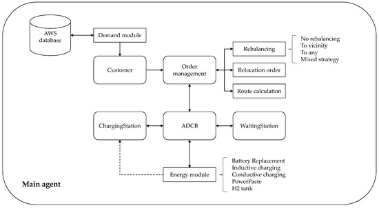
Figure 2.
Interaction between agents within the simulation model.
The individual agents shown in in Figure 2 are briefly described as follows.
Main agent: As the model’s main environment, the functions of the Main agent are as follows:
- Acting as a communication channel for other agents to interact.
- Fetching the demand data from a database using the demand module. For our model, we used an AWS database to store all generated demand scenarios and created a custom interface to access and fetch the data from the database.
- Acting as custom input interface for business input and choosing order management algorithms and energy supply strategies.
- Handling the animation view of various system components such as ADCB, waiting and charging stations, and customer population on the GIS map of the simulation environment.
- Visualizing the KPI dashboard of the entire system.
Customer agent: The “createusers()” function from the Main agent populates Customer agents based on the demand data into the simulation environment. While entering the system, a Customer agent creates an order request for an ADCB. The request is forwarded to the Order management module.
Order management: This module consists of matching, rebalancing, and route calculation algorithms. The matching algorithm assigns an ADCB to the customer and creates a custom autonomous route. The rebalancing agent calculates the imbalance of bikes in various regions and sends the available bikes to the demand locations. An investigation of different fleet management strategies is provided by Haj Salah et al. [58].
ADCB agent: The ADCB agent is modeled with the behavior of autonomous driving capability. The assigned ADCB is activated with the instructions from the Order management to serve a specific customer. The ADCB agent interacts with the rebalancing, Customer, WaitingStation, and ChargingStation agents to follow the behavioral operation of the OSABS system.
WaitingStation and ChargingStation agents: After the ADCB completes its trip, it drives autonomously to the waiting or charging station, depending on the battery status. In this study, we consider no infrastructure for the waiting station and infrastructure for the charging station based on the type of energy supply used for the ADCB. Different station distribution strategies are presented in [59].
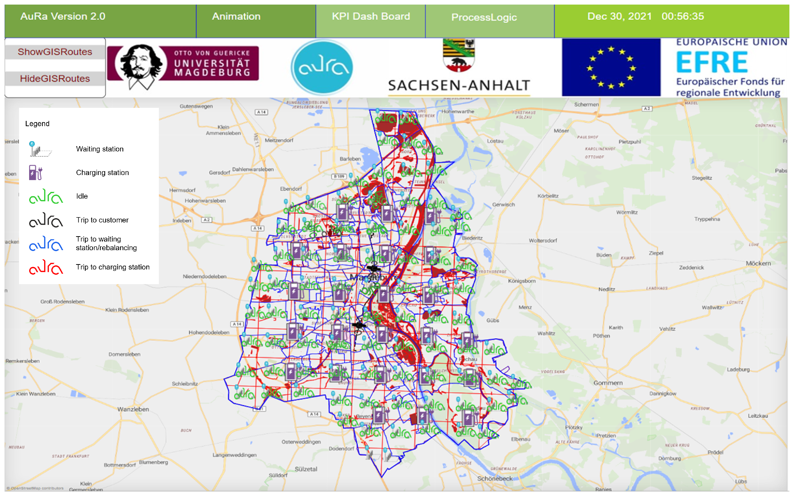
Simulation Model Animation Window: Figure 3 shows the operational view of our simulation model with ADCB driving within the operational area. Also, the animation contains charging stations and waiting stations with idle ADCB.
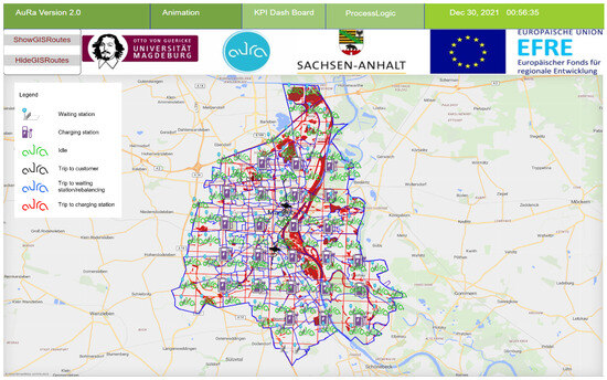
Figure 3.
Simulation animation window.
4. Demand Scenario Generation
4.1. Methodology
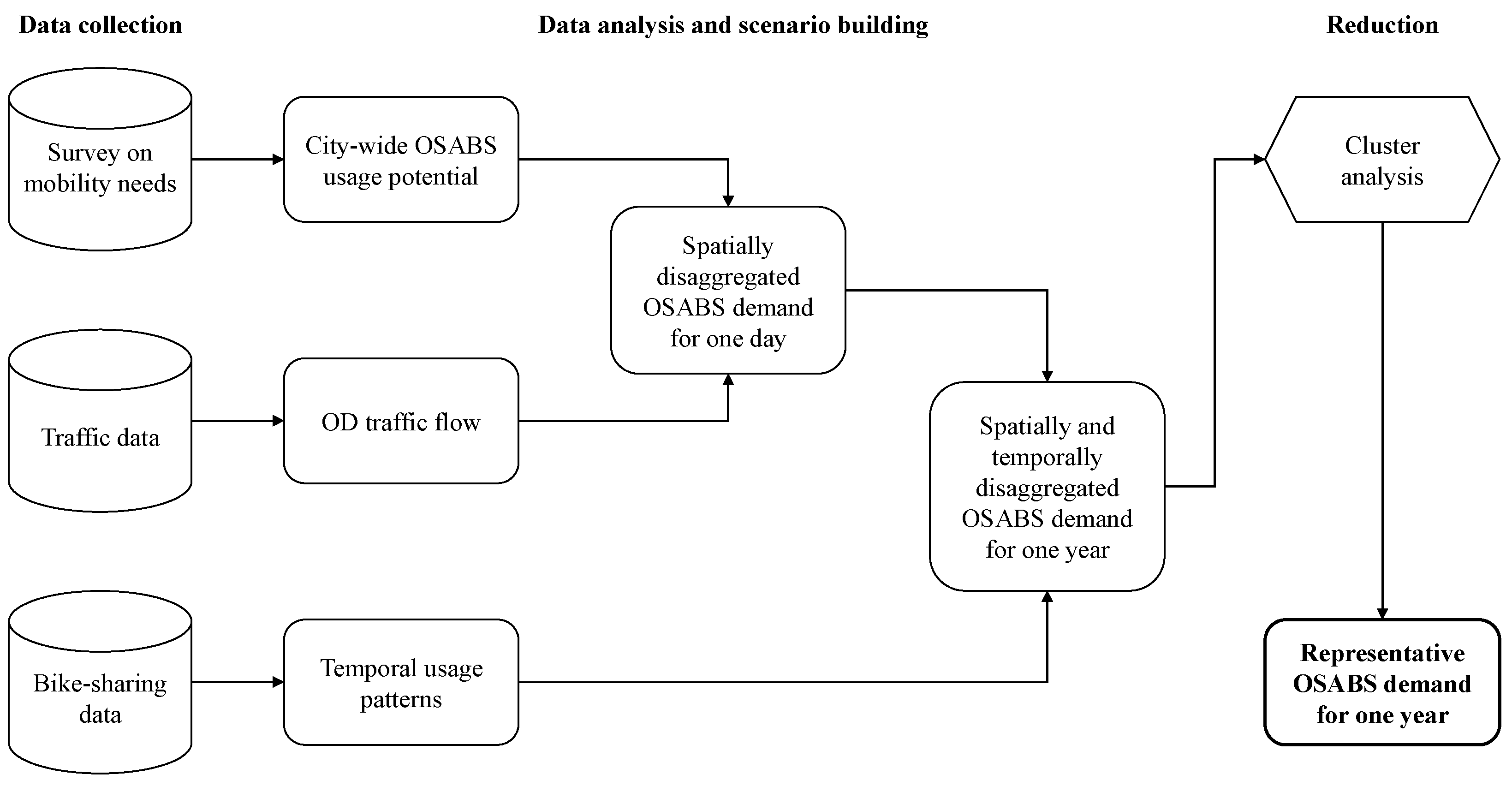
For the implementation of the proposed approach for defining OSABS demand scenarios, we used the conceptual framework outlined in Figure 4. First, we derived the city-wide usage potential of OSABS by evaluating a survey on mobility needs. In combination with existing traffic data from well-established and widely used traffic demand models (e.g., Refs. [60,61]), we determined the spatially disaggregated base demand for a statistical day. For temporal disaggregation, we derived daily, weekly, and yearly usage patterns from an existing conventional bike sharing system using generalized linear regression models. Based on the assumption that OSABS and conventional systems have similar usage patterns, we then applied the patterns to the OSABS base demand to enable hourly usage prediction for a time period of one year.
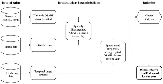
Figure 4.
Methodological approach.
Since the predicted OSABS usage is intended to serve as input for simulation models, we furthermore performed a k-medoids cluster analysis on the resulting demand scenario. The analysis aimed to map the entire course of the year with as few representative weeks as possible in order to reduce the computational effort for the simulation.
To illustrate this approach, we describe it by means of a case study for the city of Magdeburg (a large German city with approximately 235,000 residents). The datasets used for the application of our methodology are described in the subsequent chapter. For accessing, handling, and analyzing the datasets, we used the statistical softwareenvironment R (version 4.1) [62].
4.2. Dataset Description
4.2.1. Survey on Mobility Needs
The survey we evaluated for this study was part of several data collection instruments and methods developed by scientists from both logistics and human sciences collaborating on the AuRa project. They were used to investigate individual mobility needs in Magdeburg as well as the acceptability of autonomous (cargo) mobility [12,15]. Next to measures considering aspects of acceptability research, a comprehensive online survey in which a total of 1099 respondents participated between April and June 2020 [15] posed questions that access the usage potential of OSABS.
Of the participants, 50.1% were male, 49.1% were female, and 0.4% were diverse. Participants had an average age of 40.57 years ( = 16.31 years), and ages ranged from 18 to 88 years. Other analyses from this survey were previously reported in [15].
To find out more about the intention to use autonomous cargo bikes, the participants were asked how likely they were to replace conventional modes of transport with autonomous cargo bikes for various trip purposes. In addition, they were asked about their intention to use autonomous cargo bikes, what distance they would cover on average in everyday life with an autonomous cargo bike, and whether they believed OSABS to be a climate-friendly means of transport.
4.2.2. Traffic Dataset
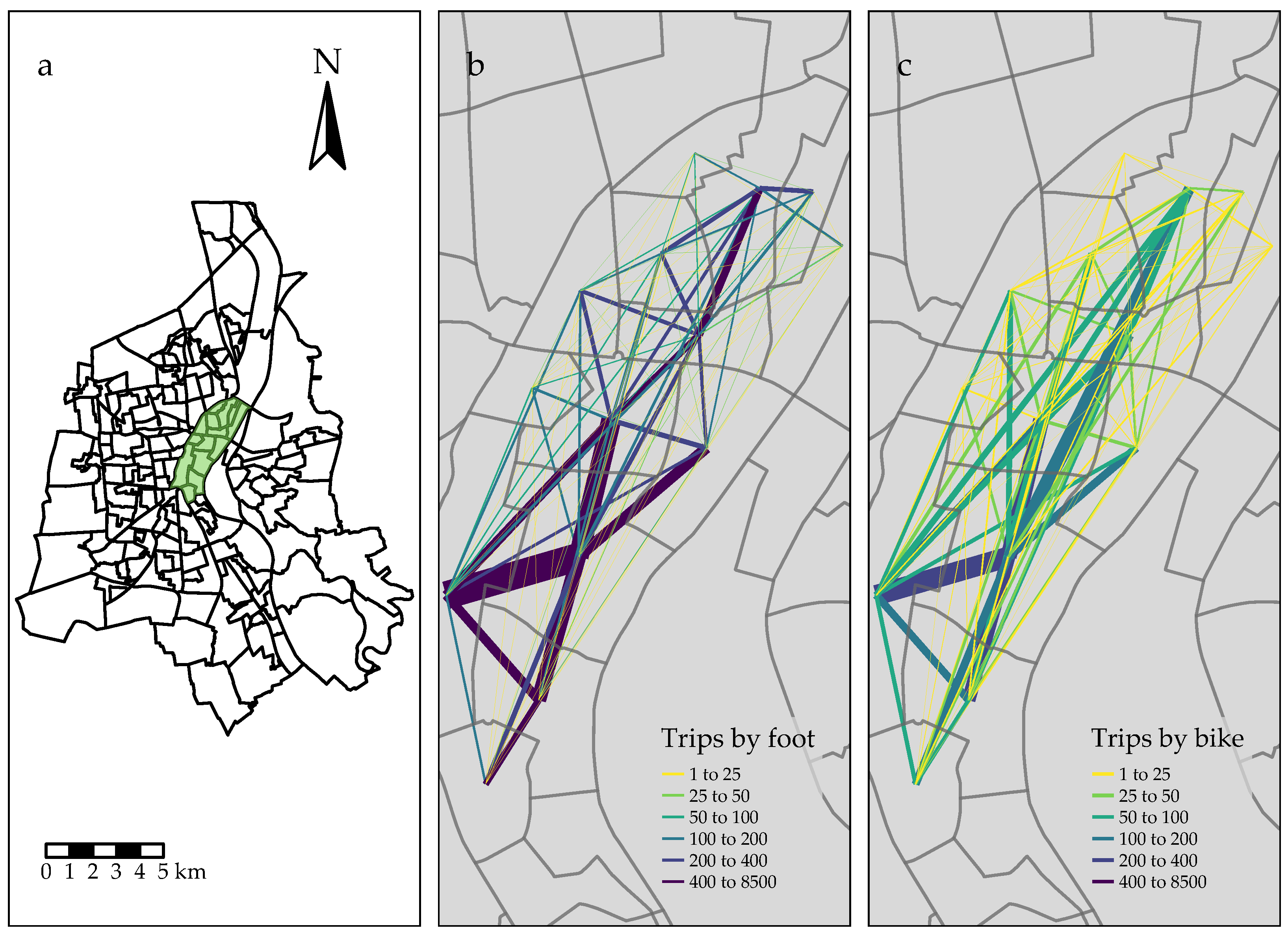
Within the framework of our case study, we used travel demand matrices provided by the municipality of Magdeburg. They contain trips for four different modes of transport, including foot, bike, car, and public transport, for a time period of one day. The matrices are structured in a way that the rows contain all trips generated from each origin and the columns contain all trips attracted from each destination. Therefore, they are often referred to as origin–destination matrices (OD-matrices). Within the matrices, a total of 182 districts evenly distributed throughout the city of Magdeburg serve as origins and destinations. In order to access the geographic location and geometry information of those districts, we used an ESRI shapefile which was also provided by the municipality of Magdeburg. A map of the city of Magdeburg as well as its districts is shown in Figure 5a. Additionally, the inner-city OD-flows for the transport modes foot and bike are shown in Figure 5b and Figure 5c, respectively.
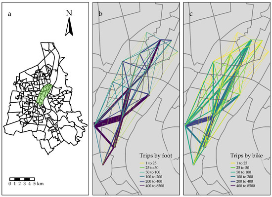
Figure 5.
(a) Magdeburg city districts (green: inner-city area). (b) Inner-city OD-flows by foot. (c) Inner-city OD-flows by bike.
In the transport sector, since travel demand matrices contain passenger or vehicle trips related to a certain period of time [60], they commonly serve as input for the development of travel demand models which are designed to model movements of road users within a transport network [61]. According to Collin [63], traffic models for a period of one day are usually related to so-called normal working days or statistical traffic days (i.e., Tuesday or Thursday), since they reflect traffic events most representatively. This also applies for the traffic demand matrices used for this study.
4.2.3. Bike Sharing Dataset
For deriving temporal bike sharing usage patterns, we investigated counts of bike rentals in a conventional public bike sharing system in Hamburg, Germany. The data were recorded from January 2014 to May 2017 and are provided by the Open-Data-Portal of Deutsche Bahn (national railway company of Germany) [64]. Although the data were collected several years ago, we chose the Hamburg bike sharing system for several reasons. First, the dataset is publicly accessible. Second, we expected both Hamburg and Magdeburg to have similar temporal characteristics in bike sharing usage due to geographic proximity. Lastly, we assume that usage patterns have not changed between 2017 and today and can therefore still be considered as granted. For each booking in the system, the dataset contains information about booking time, start and destination stations, rental duration, as well as user-related information like customer ID or technical income channel.
Since our aim was to determine usage patterns based on a full year and 2017 rental data are merely available for 5 months, we only considered bookings from 2014 to 2016. In addition, we filtered out all bookings having the same origin and destination and a rental duration of less than two minutes, as we assumed that these are due to erroneous rental processes or for maintenance purposes.
4.3. OSABS Base Demand and Beliefs
4.3.1. Assessment of OSABS as a Climate-Friendly Means of Transport and Intention to Use It
In the survey described in Section 4.2.1, two questions were used to assess whether autonomous transport bikes would be considered a climate-friendly mode of transport: (1) “In my opinion, the introduction of autonomous transport bikes brings many benefits for a climate-friendly mobility transition” and (2) “I believe that the introduction of autonomous transport bikes brings benefits for the population in the evolution towards climate-friendly transport”. Both items were answered on a five-point Likert scale with the options “strongly disagree”, “strongly disagree”, “undecided”, “strongly agree”, and “strongly agree”. Alternatively, “no answer” could be selected.
A total of 781 people answered item 1 (“Advantages for a climate-friendly change in transport”), of which 48.4% tended to agree and a further 25.9% fully agreed. Similarly, for item 2 (“Benefits for the population in the development toward climate-friendly transport”), of the 781 people who answered it, 50.1% tended to agree and another 24.3% fully agreed.
With regard to the likelihood of use, participants could indicate whether they rated their own use of the autonomous cargo bike as “not at all likely”, “rather not likely”, “undecided”, “rather likely”, or “very likely” on a five-point Likert scale. Of the 782 people who answered this item, 31.8% thought use was rather likely, and a further 12.5% thought it was very likely. A total of 23.9% were undecided.
In summary, these descriptive results shed positive light on a possible OSABS use case. More than half of the respondents perceived OSABS as a possible contribution to climate-friendly transport. And although the system did not even exist in prototype form at the time of the survey, 44.3% of respondents could imagine using it themselves. This provides a promising starting point for an application scenario.
4.3.2. Assessment of OSABS Base Demand
The evaluation of the previously described survey on mobility needs in Magdeburg showed that about 16.67% of all trips by foot, 16.49% by bike, 14.47% by public transport, and 15.65% by car are likely to be replaced by using autonomous cargo bikes. Below, these values are referred to as probability of use per mode of transport . In addition, a large proportion of respondents indicated they would travel a maximum of 10 km on an autonomous cargo bike. The exact distance distribution is shown in Table 1.

Table 1.
Stated OSABS distance limits.
To determine the traffic volume of autonomous cargo bikes for a statistical day, we calculated the number of trips replaced with OSABS by multiplying the previously obtained usage probabilities per mode of transport with OD-trips from the respective OD-matrices . In order to provide a wide range of input for any subsequent simulation models, we conducted this while distinguishing between two different scenarios:
- High scenario: A share of trips from all modes of transport, namely, foot, bike, car, and public transport, will be replaced with OSABS.
- Low scenario: A share of trips by only foot, bike, and public transport will be replaced with OSABS.
For each OD-pair, we then multiplied the resulting number of OSABS trips by the probability of use, which we derived from the trip distance and the stated distance limits from Table 1. In the following, this probability will be referred to as distance-dependent probability of use . Since no information was available on the actual starting and ending locations within origin and destination districts, it was necessary to estimate trip distances. Therefore, using shapefile and the software packages sf [65] and stplanr [66], we determined the Euclidean distance between the centroids of the respective OD-districts and multiplied it by a factor of 1.3. According to Hoerstebrock [67], this factor has proven to be a sound approximation of actual distances traveled within cities. To calculate intrazonal trips (i.e., trips within a district), for which the distance-dependent probability of use would be zero according to the above calculation, a distance of one kilometer was assumed.
In conclusion, the calculation of OSABS trips per OD-pair can be expressed via the following equations:
Since most of the calculated traffic flows were non-integer values, it was then necessary to apply an algorithm that allows for rounding the results to integer values while preserving their overall sum. To achieve this, after rounding every number down in the first step, we incrementally rounded up those numbers with the highest fractional parts until the desired sum was reached. The total OSABS demand for a statistical traffic day is 8322 trips for the high scenario and 5435 trips for the low scenario.
4.4. Temporal Disaggregation
4.4.1. Derivation of Temporal Patterns
For deriving temporal patterns, i.e., systematic variations in daily, weekly, and yearly profiles, we aggregated the conventional bike sharing demand data using one-hour intervals. Since the resulting data were typical count data, i.e., observations containing only non-negative integer values [68], we then applied count models based on generalized linear models (GLMs) to retrieve the impact of certain time-related influencing variables on the observed hourly bookings (see [68,69]).
Generalized linear models (GLMs), introduced by Nelder and Wedderburn in 1972 [70], serve as a comprehensive framework for various statistical models including linear regression, logistic regression, and Poisson regression. In mathematical terms, a GLM can be represented as [71,72] (note: In this representation, X denotes the matrix of explanatory variables. This differs slightly from the notation used by Müller [71], who uses in her formulation):
In this equation, denotes the expected value of the dependent variable Y given the explanatory variable X, represents an unknown parameter vector, and is the inverse of the link function G [73]. Unlike traditional linear regression, which is limited to normally distributed error terms, GLMs offer a more versatile approach characterized by three main components [70,72] (note: Müller’s [71] conceptualization of GLMs primarily focuses on two components: the distribution of Y and the link function, assuming the distribution of Y to be a member of the exponential family):
- A random component specifying the probability distribution for modeling the dependent variable Y, including Bernoulli, Binomial, Poisson, Geometric, Negative Binomial, Exponential, Gamma, Normal, and Inverse Gaussian distributions (see also [71]);
- A systematic component that describes the predictors (independent or explanatory variables) through a linear predictor function ;
- A link function G which relates the linear predictor to the mean of the distribution of the response variable Y.
As stated by Zeileis et al. [69], who give a comprehensive overview of regression models for count data and their application in R, the most simple distribution that can be used for modeling count data is the Poisson distribution. However, Poisson models are limited to the assumption that the variance in the model is identical to the mean [69]. Since our data appeared to be highly over-dispersed (i.e., the variance value is greater than the mean value), the application of a Poisson model was not feasible. According to Hilbe [74], a suitable way to deal with over-dispersion is to use a Negative Binomial regression model. As it is a generalization of the Poisson model, the Negative Binomial model loosens the restrictive assumption that the variance is equal to the mean [74].
Given the observed over-dispersion in our data, the Negative Binomial regression model emerged as the most fitting approach. Consequently, for the practical application of this model, we employed the R package MASS [75] for analyzing the representative bike sharing dataset.
To decide which influencing factors should serve as an input for our model, we examined the time-of-day variability in bike sharing rentals with respect to the different days of the week, as is illustrated in Figure 6.
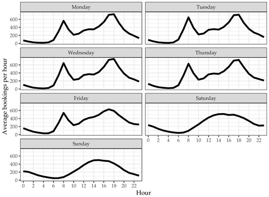
Figure 6.
Day-to-day variability in hourly bookings from conventional BSS in Hamburg, Germany.
The figure shows that the shape of daily profiles is significantly different for weekdays and weekend days. Throughout weekdays, the daily pattern is rather similar, consisting of large morning and afternoon peaks as well as a slight peak during lunchtime. However, it is noticeable that the afternoon peak on Friday is slightly below the other days. In contrast, the daily profile at weekends only shows a broad peak in the afternoon. Also, there is a high utilization at night compared to weekdays. With regard to the observations of O’Brien et al. [42] and Todd et al. [34], this indicates that the Hamburg bike sharing system user structure primarily comprises commuter and weekend leisure users.
To capture the day-to-day variability in hourly bookings within our model, we included the hour of the day and the day of the week as categorical input variables. In addition, as we could observe that the influence of daytime is different for specific days of the week, we included an interaction term between time and day of the week.
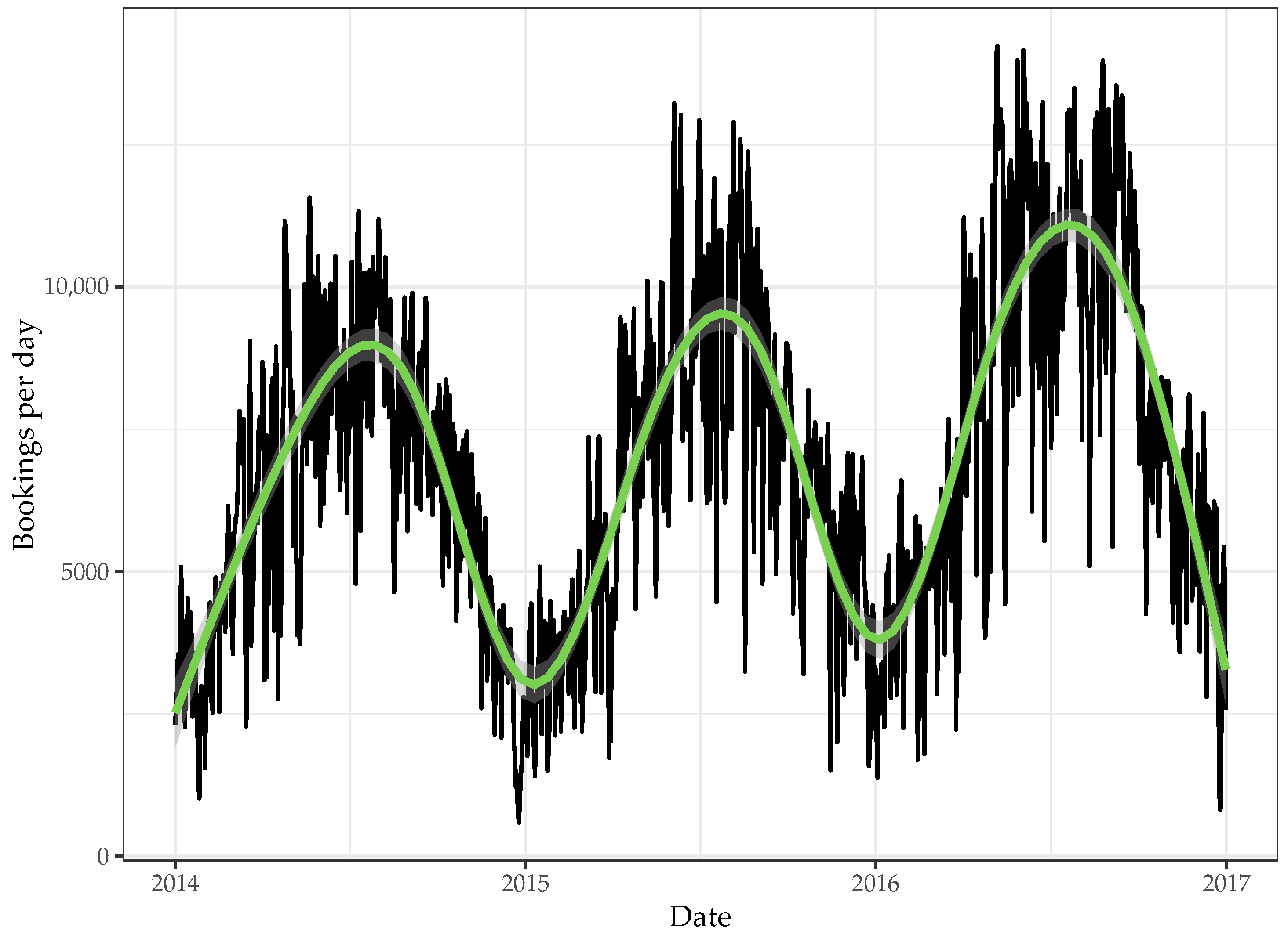
In order to access annual patterns, we furthermore analyzed the year-to-year variability in daily bookings (Figure 7). Next to a slight upward trend due to the general growth of Hamburg’s bikes sharing system [76], the figure indicates that there is a strong annual seasonal pattern (represented by the blue line). Coherent with the existing literature, this pattern consists of three periods with fewer bookings during winter, a high number of bookings during summer, and a transition phase during spring and autumn with growing and declining booking numbers, respectively.

Figure 7.
Year-to-year variability in daily bookings from conventional BSS in Hamburg, Germany (black: observed bookings; green: smoothed conditional means).
As the pattern is repeated each year, we assume that those three periods reflect the general pattern of annual bike sharing usage. However, neither the associated seasons nor the respective months provide a sufficient temporal granularity to also represent any short-term variations within the annual course. Hence, we included week numbers as a categorical variable in our model since this interval is short enough to represent fluctuations but long enough to keep the number of input variables used for the regression model within reasonable limits. In summary, the following explanatory variables were included in the model:
- Week number (reference variable: calendar week 1);
- Weekday (reference variable: Monday);
- Time of day (reference variable: hour 0);
- Interaction term between weekday and time of day.
In contrast to the uniform pattern of annual seasonality, Figure 7 also shows that the frequency of the daily seasonality is rather irregular for the different years. In order to reveal the key temporal patterns, we consolidated the three-year booking data into a dataset consisting of hourly booking figures for only one year. We performed this by averaging the hourly bookings of each corresponding hour over the three years. This dataset is called the representative bike sharing dataset as follows.
The results of our negative binomial model applied to the representative bike sharing dataset are presented in Table A1 (Appendix A.1). As this is common in the recent literature regarding the influence of temporal factors on bike sharing rentals (e.g., Refs. [11,19,25,41,43,51,53]), we used Nagelkerke’s Pseudo-R [77] to measure goodness of fit.
Table A1 shows that our model has a very high fit, as the Pseudo-R value is 0.94443. This indicates that nearly 95% of the variation in hourly bike sharing rentals can be explained using the variables used within the model. As expected, the coefficients for week-related dummy variables show that the number of trips is increased for mid-year weeks compared to weeks at the beginning or end of the year. Furthermore, since we included the interaction between weekdays and the time of the day, the results demonstrate that the regression model enables the estimation of weekday and weekend peaks. Another finding is that the influence on hourly rentals relative to the reference category is mostly not significant for the interaction between weekdays and nighttime hours. We explain this by the fact that there is hardly any difference between the nightly booking numbers on weekdays.
4.4.2. Cluster Analysis
To enable temporal disaggregation, an alternative approach could have been to directly apply the results of our regression analysis to the previously determined OSABS base demand. However, as we aimed to provide hourly demand data for a time period of one year for two different scenarios (i.e., low and high scenario), this would have led to two datasets each containing hourly rentals for 52.143 individual weeks (or 52 weeks plus one day). Thus, for reproducing the annual OSABS traffic flows within a simulation model, it would be required to simulate 8760 h (52.143 weeks · 7 days · 24 h) of OSABS usage for each scenario.
Since this would involve an unreasonable computational effort, we applied a cluster analysis to the representative bike sharing dataset. Within the analysis, we used the k-medoids clustering technique proposed by Kaufmann and Rousseeuw [78], as it is more robust to noise and outliers than standard k-means clustering. For the technical implementation in R, we used the cluster package [79]. The aim of this analysis was to identify similarities in demand profiles of certain weeks and to group them into clusters accordingly. We associated each calendar week with the number of the cluster in which it was located. Instead of the individual week numbers, we then used the cluster numbers as categorical input variables for our regression model.
In order to find the optimal number of clusters, we conducted several regression models using different cluster sizes and compared them to the initial model. For comparing the models, we used the Akaike information criterion (AIC) [80] and root mean square error (RMSE). Table 2 shows that the optimal cluster size is eight, since the performance of the according regression model is quite similar compared to the initial model. In addition, as shown in Table A2 (Appendix A.2), the -regression model provides a very high fit with a Pseudo-R of 0.94235.

Table 2.
Comparison of models with different cluster sizes as categorical input variables.
The performance of our models is further illustrated in the following charts. Figure 8 compares the observed hourly bookings (representative BSS dataset) for different weekdays, namely, Monday to Thursday, Friday, and Saturday to Sunday, against the values determined from the regression models.
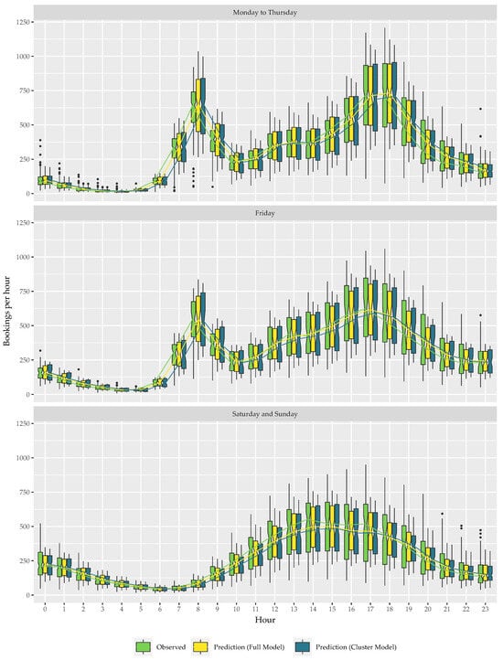
Figure 8.
Comparison of observed and predicted values for daily bookings.
The diagram effectively demonstrates that these models are highly proficient in replicating the daily fluctuations in hourly bookings. Nonetheless, it is worth noting that while these models are largely accurate, they have a slight tendency to underestimate peak demand and overestimate periods of lower demands.
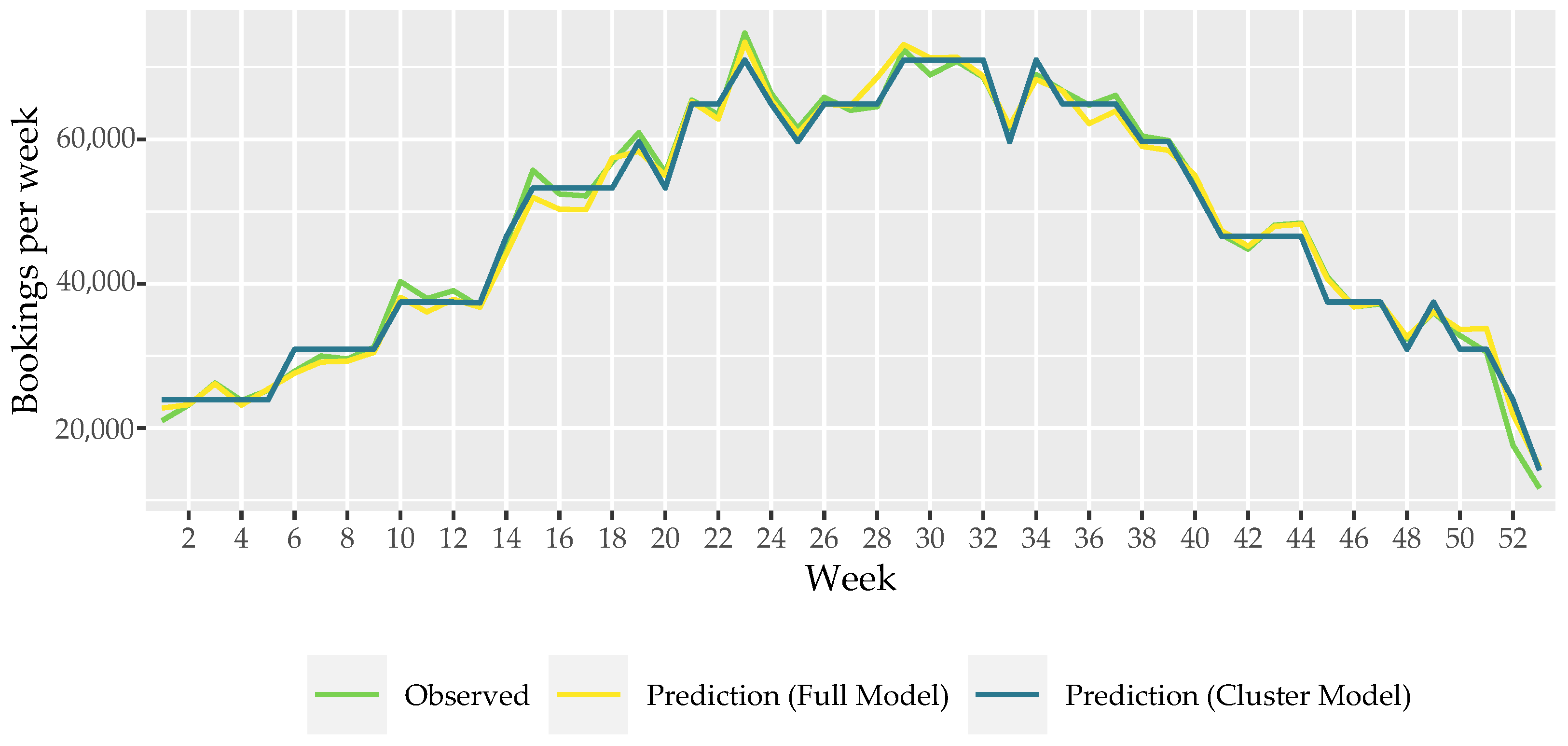
Figure 9 additionally demonstrates that both the Full Model and the Cluster Model accurately represent the annual patterns. While the Full Model slightly outperforms in reflecting short-term changes, it is noteworthy that the overall course is well reproduced by both models. Notably, the less precise representation of short-term fluctuations by the Cluster Model is not inherently disadvantageous. These fluctuations vary across different years, indicating that a perfect replication may not be necessary or even desirable for accurate modeling. Thus, the Cluster Model efficiently balances simulation effort with quality of results.
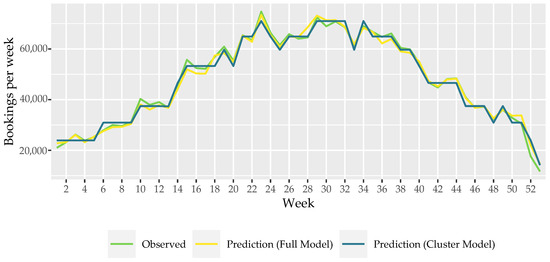
Figure 9.
Comparison of observed and predicted values for weekly bookings.
As we could prove that it is sufficient to model annual patterns using only eight representative weeks, we used the results from the -regression model for the temporal disaggregation of OSABS base demand. An overview of the assignment of the clusters to the actual calendar weeks is presented in Table 3.

Table 3.
Represented calendar weeks.
In terms of reproducing the annual OSABS traffic flows within a simulation model, this represents a reduction in computational effort of almost 85%, as it is only necessary to simulate 1344 h (8 weeks · 7 days · 24 h) of OSABS usage for each scenario. To extrapolate these results to an entire year, the resulting representative weeks (C1 to C8) can be combined according to the represented calendar weeks in Table 3.
5. Modeling Results
Since the regression coefficients are linked with the model intercept, they could not be directly applied to the OSABS base demand. Therefore, we needed to develop a methodology for effectively transferring temporal patterns to the new system based on the following assumptions:
The k8-regression model’s intercept is 36.07, and the average value of observed hourly bookings within the data is 288.14. From this, we can derive an intercept–mean ratio of 0.125 for the model. Moreover, given that the OSABS base demand for a statistical day, i.e., the average value for daily bookings, is 8322 trips for the high scenario and 5435 for the low scenario, we can calculate average values for hourly OSABS bookings of 346.75 and 226.46 for the high and low scenarios, respectively. Hence, by implementing the model’s intercept–mean ratio in OSABS, we derive intercept values of 43.34 and 28.31 for the high and low scenarios, respectively.
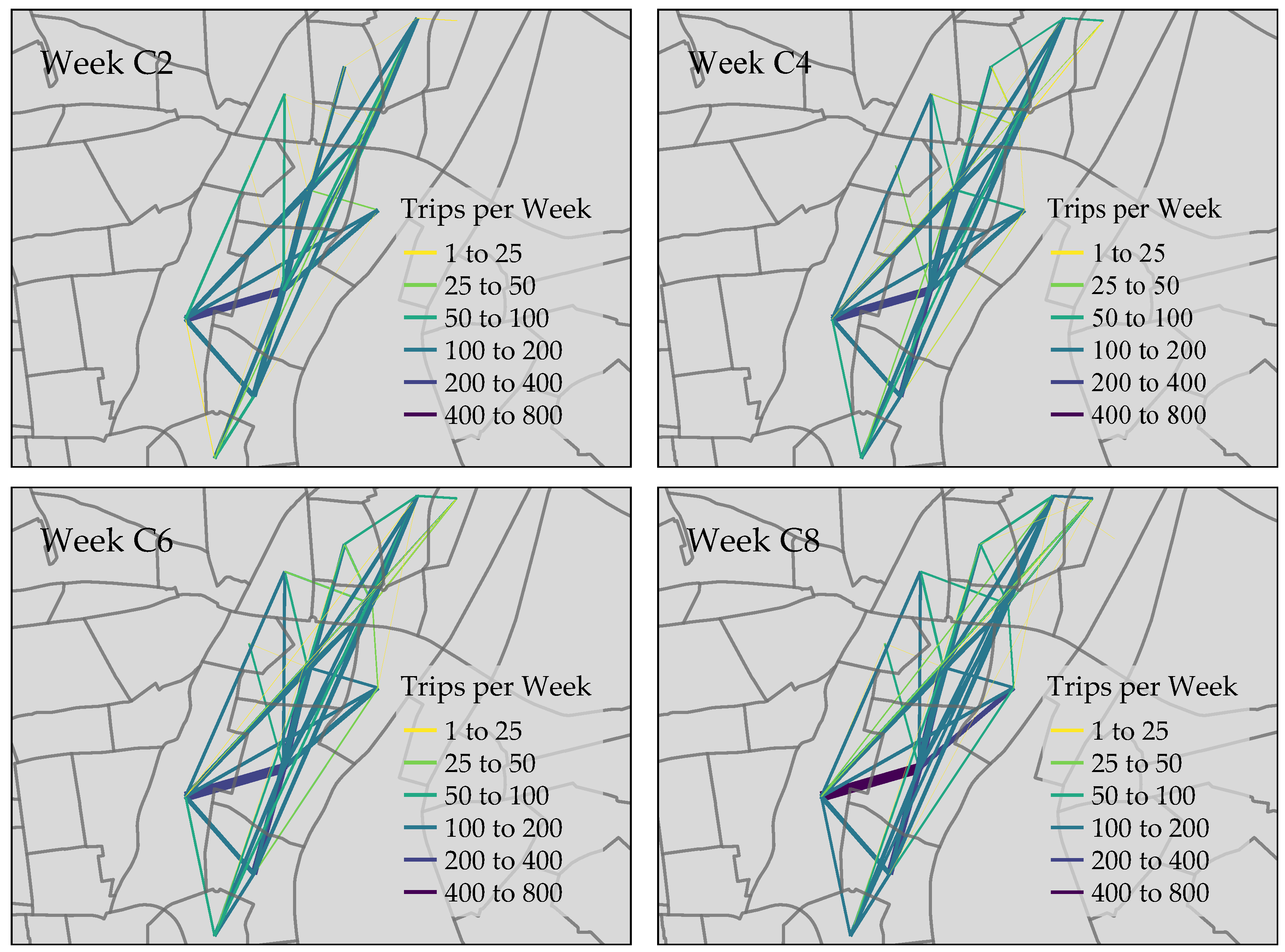
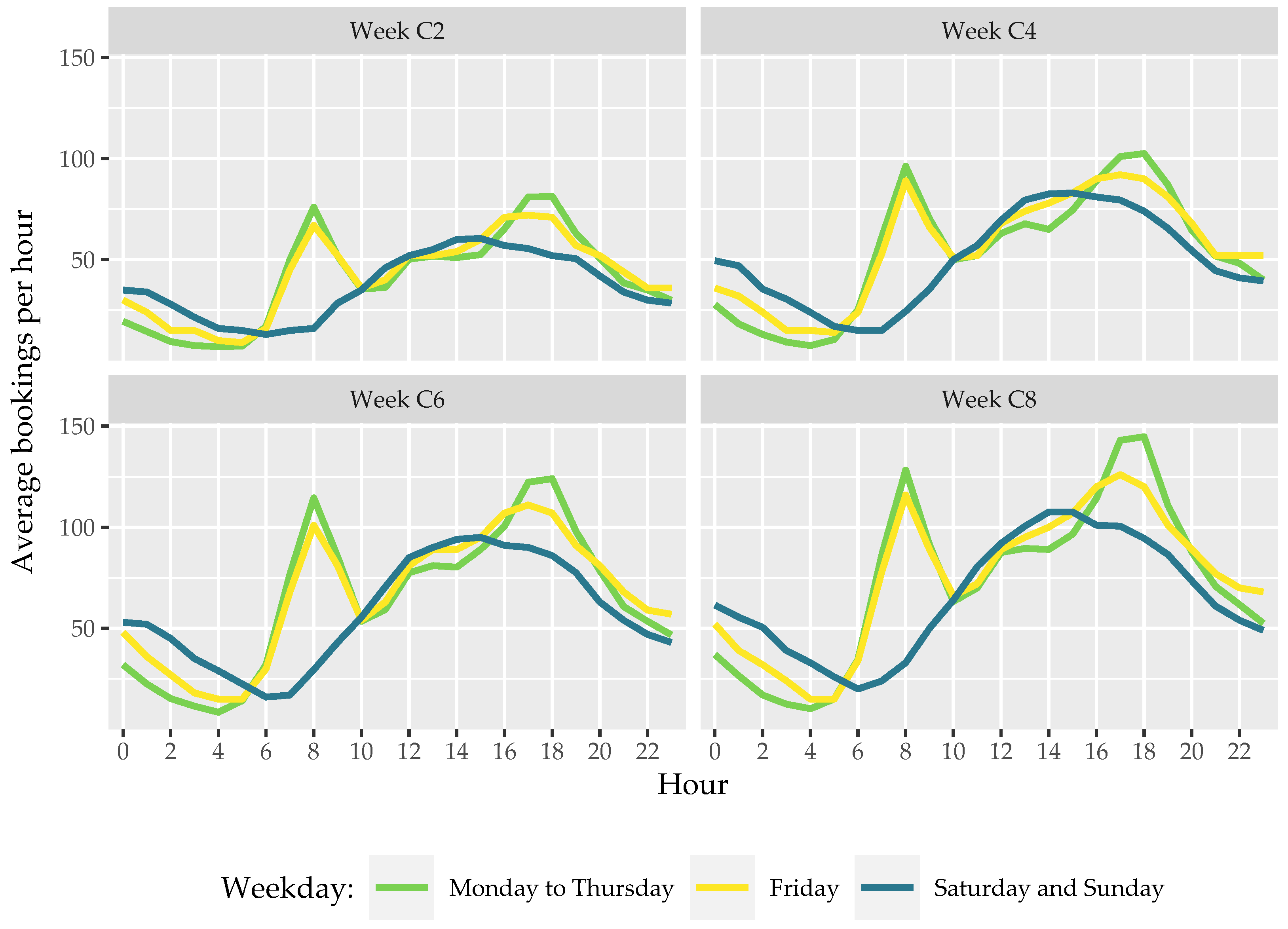
Based on these assumptions, we calculate the hourly OSABS traffic flow in Magdeburg for each of the eight representative weeks. An extract of the results is pictured in Figure 10 and Figure 11, which show predicted weekly OD-traffic flows for the inner-city area of Magdeburg as well as average hourly bookings for Monday to Thursday, Friday, and Saturday to Sunday.
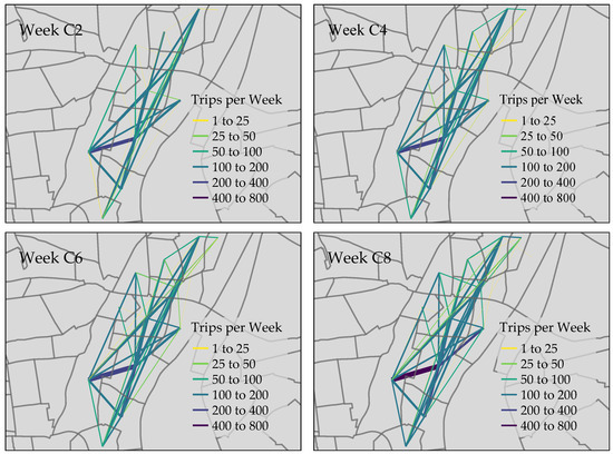
Figure 10.
Predicted weekly OSABS OD-traffic flows for Magdeburg inner-city area.
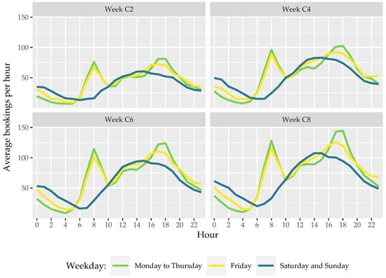
Figure 11.
Predicted hourly bookings.
As expected, the figures indicate increased OSABS utilization in weeks C6 and C8, as they represent calendar weeks with higher average temperatures compared to the calendar weeks represented by weeks C2 and C4, hence replicating annual BSS usage patterns. Moreover, Figure 10 indicates that our approach enables the prediction of OSABS traffic flows with high spatial granularity. Further, Figure 11 shows that the approach enables accurate reproducibility of previously determined day-to-day variability in hourly bookings.
A crucial aspect of our study was validating the model. We compared our model’s predictions for OSABS in Magdeburg with characteristic data from existing bike sharing systems determined by Todd et al. [34] (Table 4). This comparison served as an indirect validation method, providing a benchmark for assessing our model’s viability in real-world scenarios. As Table 4 demonstrates, our model predicts higher OSABS utilization in Magdeburg compared to conventional BSS in similar-sized cities.

Table 4.
Characteristic BSS data (based on [34]).
However, the slightly higher predicted OSABS figures are justifiable given its distinct advantages over conventional BSS. Firstly, OSABS extends the reach of bike sharing services to less dense urban areas. While traditional BSS primarily operates in densely populated, central city locations, OSABS allows for effective operation throughout the entire city, including peripheral areas, significantly expanding the potential user base and thus contributing to the higher predicted usage figures. Secondly, OSABS’s mobility-as-a-service feature, which enables users to summon vehicles directly to their location, greatly enhances user convenience and thus system utilization. Further, the ability to transport goods adds a valuable dimension to the service, attracting a wider range of users, including those who need to carry items that would be difficult with a standard bike. This feature is likely to appeal to a diverse demographic, further boosting the system’s utilization.
6. Discussion and Future Work
The resulting hourly booking figures are represented as OD-matrices and can be used directly for the OSABS simulation model. In the realm of simulation, the generated demand patterns serve as valuable input, contributing to the design and implementation of various strategies.
Firstly, the implementation of suitable order management strategies, especially rebalancing algorithms, benefits from the predicted spatial and temporal patterns, leading to enhanced operational efficiency and customer satisfaction. Additionally, our methodology provides guidance for the placement of OSABS stations. By accurately predicting traffic flows with high spatial granularity, we can identify areas of high demand and strategically position stations to meet this demand, thus optimizing resource allocation and improving service availability. Furthermore, our approach supports the selection of suitable energy supply technologies. The ability to anticipate OSABS utilization patterns, particularly during periods of increased usage, aids in making informed decisions about the types of energy supply technologies that would be most efficient and sustainable.
A further advantage of the proposed methodology lies in its wide applicability to other cities or use cases, as the data used, i.e., bike sharing data (in general or for the city itself) and OD-matrices (most often for larger cities), are widely available. Moreover, the survey on usage probabilities and distance limits can be conducted with little preparation and survey effort. Hence, in terms of conventional BSS, city authorities could use our approach to straightforwardly determine efficient locations for bike docking stations, which not only would ensure that bikes are available where and when they are needed but could also prevent issues such as overcrowding at certain stations. Similarly, system operators could use our demand scenarios to optimize bike distribution, reducing the amount of time and resources spent on repositioning bikes. Hence, through promoting the adoption of (conventional) bike sharing systems, our research may also help to drive a shift towards more sustainable modes of transportation, resulting in reduced carbon emission and air pollution in cities, but also in improved public health and overall quality of stay.
While providing new insights into the generation of demand scenarios for novel transportation systems, our study also raises the need for additional research.
One primary challenge is the theoretical nature of our model coupled with the lack of real-world OSABS data. This has led to a reliance on indirect validation methods, where we compare our model’s predictions with existing bike sharing systems data. The comparison suggested higher predicted OSABS utilization in Magdeburg, which we attribute to the unique features of OSABS, such as its extended reach and mobility-as-a-service offerings. While retrieving reasonable results from indirect validation, the integration of real-world OSABS data in future studies and hence the direct validation of our predictions remains a pivotal task.
Further, in our analysis, we applied annual usage patterns to represent long-term fluctuations in demand. To enhance the model’s accuracy in capturing short-term demand fluctuations, future work could involve the integration of real-time traffic data, weather conditions, and information about special events into the demand forecasting process. This would allow for a more dynamic and responsive model, better suited to the complexities of urban transportation.
An additional limitation arises from our model’s reliance on traffic zones for predicting demand, without giving the exact position for single requests. In line with findings from Krause et al. [12] and Kastner et al. [15], we aim to refine the spatial detail of our demand forecasts in future iterations of our research by incorporating land use, sociodemographic information, and different trip purposes.
Moreover, the extrapolation of bike sharing patterns from Hamburg to Magdeburg, while a necessary simplification for our case study, may not fully capture the specific dynamics of the Magdeburg area. This limitation affects the temporal disaggregation of the predicted OSABS data for Magdeburg but does not impinge on the broader applicability of our methodology to other urban contexts. Enhancing data availability could significantly improve the results of our case study, underlining the potential of our methodology when applied with context-specific data.
Lastly, the application of advanced machine learning algorithms in future research could lead to more accurate demand predictions and a reduction in the computational effort required for simulating annual traffic flows. However, the challenge of data availability remains a significant hurdle. Comprehensive data collection can be time-consuming and costly, potentially affecting the ease of transferring our methodology to diverse locations. Addressing this challenge may require collaborative efforts between various stakeholders, including cities, system operators, universities, and research institutions.
7. Conclusions
In this paper, we presented a data-driven approach for defining demand scenarios for OSABS. We described the implementation of our approach by means of a case study in the city of Magdeburg. In particular, we assessed the potential utilization of OSABS by analyzing a survey on mobility needs. Our analysis indicated that approximately 15% to 16% of all inner-city trips could be replaced by OSABS, with the majority of respondents viewing OSABS as an environmentally friendly transportation alternative.
Furthermore, we employed existing travel demand matrices for spatial disaggregation and usage patterns derived from a conventional bike sharing system via a negative binomial model for temporal disaggregation. As the model fit indicates, with week number, weekday, time of day, and an interaction term between weekday and time of day as input variables, we could explain nearly 95% of the variation in hourly bike sharing within the data.
In addition, since the derived demand scenarios are intended to be used as inputs for an agent-based simulation model, we performed a cluster analysis to identify similar patterns in the annual usage profile and reduce data size. Through cluster analysis, we demonstrated that annual bike sharing usage patterns can be modeled using a combination of eight representative weeks, resulting in nearly an 85% reduction in computational effort.
In summary, our study contributes to existing research by proposing a new methodology for generating demand scenarios for novel transportation systems with high spatial and temporal granularity. The generated demand scenarios can be integrated into an agent-based simulation model, enabling us to explore various facets of the new transportation system in the context of the city of Magdeburg. However, our approach has wider applicability and can be adapted for other cities or for estimating the potential utilization of other active and public transportation systems such as conventional bike sharing schemes, therefore encouraging active mobility.
Author Contributions
Conceptualization, M.K. and T.A.; data curation, M.K. and K.K.; formal analysis, M.K. and K.K.; funding acquisition, K.K. and T.A.; methodology, M.K.; project administration, T.A.; supervision, T.A.; validation, M.K., V.D.M., K.K. and T.A.; visualization, M.K.; writing—original draft preparation, M.K., V.D.M. and K.K.; writing—review and editing, M.K. All authors have read and agreed to the published version of the manuscript.
Funding
This research was part of the research project AuRa (Autonomes Rad, (Eng. Autonomous Bicycle)) funded by the federal state of Saxony-Anahlt, Germany, and the European Regional Development Funds (EFRE, 2014–2020), project number 19-15003/004.
Informed Consent Statement
For the conducting of the survey, all ethical principles were observed in accordance with the guidelines of the German Research Foundation (DFG, https://www.dfg.de/en/research_funding/faq/faq_humanities_social_science/index.html, accessed 2 January 2020). Within the survey, informed consent was obtained from all subjects involved in the study.
Data Availability Statement
A publicly available dataset on the conventional bike sharing system in Hamburg, Germany, was analyzed in this study. This data can be found here: https://data.deutschebahn.com/dataset/data-call-a-bike.html (accessed on 1 March 2022). Restrictions apply to the availability of the traffic data. The data were obtained from the municipality of Magdeburg and are available from the authors with the permission of the municipality of Magdeburg. Further, additional data resulting from the survey on mobility needs are available on request from the corresponding author. The data are not publicly available due to privacy and data usage agreements.
Acknowledgments
We express our gratitude to the transportation planning department of the city of Magdeburg, Germany, for providing the travel demand matrices and shapefiles.
Conflicts of Interest
The authors declare no conflict of interest.
Abbreviations
The following abbreviations are used in this manuscript:
| ADCB | autonomous driving cargo bike |
| AIC | Akaike information criterion |
| BSS | bike sharing system |
| OCC | Operations Control Center |
| OSABS | on-demand, shared-use, self-driving cargo bikes service |
| RMSE | root mean square error |
Appendix A
Appendix A.1
The subsequent Table A1 contains the estimated parameter values for the regression model described in Section 4.4.1. The following explanatory variables were included in the model:
- Week number (weeknum1 … weeknum53);
- Weekday (Monday … Sunday);
- Time of day (hour00 … hour23);
- Interaction term between weekday and time of day (Monday × hour00 … Sunday × hour23).

Table A1.
Estimated parameter values for Negative Binomial model (Full Model).
Table A1.
Estimated parameter values for Negative Binomial model (Full Model).
| Parameter | exp(Estimate) | 2.5% | 97.5% | z-Value | p-Value |
|---|---|---|---|---|---|
| Intercept | 34.26298 | 31.76959 | 36.95205 | 91.67588 | 0 |
| weeknum2 | 1.02011 | 0.969 | 1.07391 | 0.75919 | 0.44774 |
| weeknum3 | 1.14702 | 1.08985 | 1.2072 | 5.25779 | 0 |
| weeknum4 | 1.0181 | 0.96709 | 1.0718 | 0.68407 | 0.49393 |
| weeknum5 | 1.11568 | 1.06 | 1.17428 | 4.19079 | 0.00003 |
| weeknum6 | 1.21136 | 1.15111 | 1.27477 | 7.36623 | 0 |
| weeknum7 | 1.28 | 1.21647 | 1.34685 | 9.50437 | 0 |
| weeknum8 | 1.28539 | 1.2216 | 1.3525 | 9.66757 | 0 |
| weeknum9 | 1.33841 | 1.27209 | 1.40819 | 11.24165 | 0 |
| weeknum10 | 1.67394 | 1.59163 | 1.76051 | 20.02514 | 0 |
| weeknum11 | 1.58455 | 1.5065 | 1.66665 | 17.85964 | 0 |
| weeknum12 | 1.66135 | 1.57964 | 1.74729 | 19.72687 | 0 |
| weeknum13 | 1.61856 | 1.53876 | 1.70248 | 18.66883 | 0 |
| weeknum14 | 1.93974 | 1.84477 | 2.03959 | 25.87019 | 0 |
| weeknum15 | 2.28094 | 2.16976 | 2.39783 | 32.34076 | 0 |
| weeknum16 | 2.20978 | 2.10198 | 2.32311 | 31.07184 | 0 |
| weeknum17 | 2.20586 | 2.09825 | 2.319 | 31.00083 | 0 |
| weeknum18 | 2.52049 | 2.39793 | 2.64932 | 36.34807 | 0 |
| weeknum19 | 2.56214 | 2.4376 | 2.69304 | 37.00693 | 0 |
| weeknum20 | 2.41433 | 2.29681 | 2.53786 | 34.61958 | 0 |
| weeknum21 | 2.86377 | 2.72491 | 3.0097 | 41.49003 | 0 |
| weeknum22 | 2.75786 | 2.62402 | 2.89851 | 39.97045 | 0 |
| weeknum23 | 3.22538 | 3.06937 | 3.38932 | 46.29455 | 0 |
| weeknum24 | 2.87377 | 2.73444 | 3.0202 | 41.63074 | 0 |
| weeknum25 | 2.66936 | 2.53973 | 2.80561 | 38.65667 | 0 |
| weeknum26 | 2.84903 | 2.71087 | 2.99423 | 41.28189 | 0 |
| weeknum27 | 2.83947 | 2.70176 | 2.98419 | 41.14625 | 0 |
| weeknum28 | 3.01198 | 2.86609 | 3.1653 | 43.52709 | 0 |
| weeknum29 | 3.21143 | 3.05608 | 3.37468 | 46.11924 | 0 |
| weeknum30 | 3.12983 | 2.97835 | 3.28901 | 45.0782 | 0 |
| weeknum31 | 3.13423 | 2.98255 | 3.29364 | 45.13509 | 0 |
| weeknum32 | 3.01874 | 2.87253 | 3.17239 | 43.61758 | 0 |
| weeknum33 | 2.71723 | 2.58533 | 2.85587 | 39.37255 | 0 |
| weeknum34 | 2.99858 | 2.85333 | 3.15123 | 43.34698 | 0 |
| weeknum35 | 2.92831 | 2.78639 | 3.07746 | 42.38946 | 0 |
| weeknum36 | 2.73051 | 2.59798 | 2.86981 | 39.56896 | 0 |
| weeknum37 | 2.80666 | 2.67051 | 2.94974 | 40.67756 | 0 |
| weeknum38 | 2.59161 | 2.46567 | 2.72398 | 37.46689 | 0 |
| weeknum39 | 2.56738 | 2.44259 | 2.69855 | 37.0892 | 0 |
| weeknum40 | 2.41534 | 2.29777 | 2.53893 | 34.63645 | 0 |
| weeknum41 | 2.07896 | 1.97737 | 2.18576 | 28.63293 | 0 |
| weeknum42 | 1.9848 | 1.88769 | 2.0869 | 26.78454 | 0 |
| weeknum43 | 2.10549 | 2.00264 | 2.21361 | 29.13916 | 0 |
| weeknum44 | 2.1187 | 2.01522 | 2.22748 | 29.389 | 0 |
| weeknum45 | 1.78337 | 1.69585 | 1.87541 | 22.53153 | 0 |
| weeknum46 | 1.61476 | 1.53527 | 1.69837 | 18.6041 | 0 |
| weeknum47 | 1.64079 | 1.56005 | 1.7257 | 19.23495 | 0 |
| weeknum48 | 1.43213 | 1.36134 | 1.5066 | 13.88654 | 0 |
| weeknum49 | 1.58481 | 1.50674 | 1.66692 | 17.86604 | 0 |
| weeknum50 | 1.47809 | 1.40511 | 1.55486 | 15.12477 | 0 |
| weeknum51 | 1.48365 | 1.4104 | 1.5607 | 15.27207 | 0 |
| weeknum52 | 0.96206 | 0.91374 | 1.01295 | −1.47079 | 0.14135 |
| weeknum53 | 1.08627 | 1.02309 | 1.15334 | 2.70687 | 0.00679 |
| Tuesday | 1.21511 | 1.1074 | 1.33328 | 4.11433 | 0.00004 |
| Wednesday | 1.47684 | 1.34758 | 1.61848 | 8.34384 | 0 |
| Thursday | 1.7986 | 1.64238 | 1.96968 | 12.66232 | 0 |
| Friday | 2.20075 | 2.01084 | 2.40859 | 17.13148 | 0 |
| Saturday | 3.15338 | 2.88372 | 3.44827 | 25.17958 | 0 |
| Sunday | 2.93707 | 2.68456 | 3.21334 | 23.49004 | 0 |
| hour1 | 0.63309 | 0.57451 | 0.69765 | −9.22725 | 0 |
| hour2 | 0.35303 | 0.31826 | 0.39159 | −19.68451 | 0 |
| hour3 | 0.24193 | 0.21673 | 0.27006 | −25.28759 | 0 |
| hour4 | 0.21409 | 0.19132 | 0.23958 | −26.85745 | 0 |
| hour5 | 0.35319 | 0.31841 | 0.39176 | −19.67729 | 0 |
| hour6 | 1.17402 | 1.06978 | 1.28842 | 3.38174 | 0.00072 |
| hour7 | 4.20006 | 3.84143 | 4.59218 | 31.51366 | 0 |
| hour8 | 8.05472 | 7.3723 | 8.80031 | 46.18864 | 0 |
| hour9 | 4.88454 | 4.46841 | 5.33943 | 34.91168 | 0 |
| hour10 | 2.96949 | 2.71425 | 3.24873 | 23.73552 | 0 |
| hour11 | 3.32317 | 3.03822 | 3.63486 | 26.25496 | 0 |
| hour12 | 4.45261 | 4.07276 | 4.86789 | 32.82732 | 0 |
| hour13 | 4.90057 | 4.48309 | 5.35693 | 34.98547 | 0 |
| hour14 | 4.84373 | 4.43103 | 5.29488 | 34.72273 | 0 |
| hour15 | 5.81653 | 5.32211 | 6.35688 | 38.84665 | 0 |
| hour16 | 7.34448 | 6.72172 | 8.02495 | 44.10652 | 0 |
| hour17 | 9.74475 | 8.92038 | 10.64529 | 50.4847 | 0 |
| hour18 | 9.9338 | 9.09356 | 10.85167 | 50.91803 | 0 |
| hour19 | 6.94375 | 6.35464 | 7.58746 | 42.84101 | 0 |
| hour20 | 4.53713 | 4.15018 | 4.96016 | 33.25051 | 0 |
| hour21 | 3.27708 | 2.99599 | 3.58454 | 25.94193 | 0 |
| hour22 | 2.56025 | 2.3394 | 2.80194 | 20.42573 | 0 |
| hour23 | 1.80233 | 1.6452 | 1.97445 | 12.65788 | 0 |
| Tuesday × hour1 | 0.95022 | 0.82956 | 1.08842 | −0.73708 | 0.46108 |
| Wednesday × hour1 | 1.0005 | 0.87547 | 1.14339 | 0.00735 | 0.99414 |
| Thursday × hour1 | 0.9972 | 0.87369 | 1.13818 | −0.04152 | 0.96688 |
| Friday × hour1 | 1.14338 | 1.00323 | 1.30311 | 2.00833 | 0.04461 |
| Saturday × hour1 | 1.34922 | 1.18582 | 1.53513 | 4.54771 | 0.00001 |
| Sunday × hour1 | 1.50372 | 1.3209 | 1.71185 | 6.16798 | 0 |
| Tuesday × hour2 | 0.8832 | 0.76379 | 1.02128 | −1.67584 | 0.09377 |
| Wednesday × hour2 | 0.92873 | 0.80571 | 1.07055 | −1.01973 | 0.30786 |
| Thursday × hour2 | 1.04719 | 0.9108 | 1.20399 | 0.64765 | 0.51721 |
| Friday × hour2 | 1.3587 | 1.18477 | 1.55818 | 4.38582 | 0.00001 |
| Saturday × hour2 | 1.77705 | 1.55317 | 2.03319 | 8.36874 | 0 |
| Sunday × hour2 | 2.15356 | 1.8811 | 2.46549 | 11.11537 | 0 |
| Tuesday × hour3 | 0.78137 | 0.66873 | 0.91297 | −3.10645 | 0.00189 |
| Wednesday × hour3 | 0.82919 | 0.71274 | 0.96466 | −2.4259 | 0.01527 |
| Thursday × hour3 | 0.99725 | 0.86077 | 1.15537 | −0.03663 | 0.97078 |
| Friday × hour3 | 1.31706 | 1.14086 | 1.52047 | 3.75843 | 0.00017 |
| Saturday × hour3 | 1.84739 | 1.60544 | 2.1258 | 8.56976 | 0 |
| Sunday × hour3 | 2.3269 | 2.02185 | 2.67798 | 11.77907 | 0 |
| Tuesday × hour4 | 0.63318 | 0.53798 | 0.74523 | −5.49707 | 0 |
| Wednesday × hour4 | 0.64155 | 0.54764 | 0.75155 | −5.49712 | 0 |
| Thursday × hour4 | 0.75317 | 0.64634 | 0.87765 | −3.63216 | 0.00028 |
| Friday × hour4 | 0.97179 | 0.8379 | 1.12708 | −0.37833 | 0.70518 |
| Saturday × hour4 | 1.52429 | 1.32075 | 1.75919 | 5.76421 | 0 |
| Sunday × hour4 | 1.98239 | 1.71782 | 2.28769 | 9.36317 | 0 |
| Tuesday × hour5 | 0.78739 | 0.68015 | 0.91153 | −3.20011 | 0.00137 |
| Wednesday × hour5 | 0.66987 | 0.57946 | 0.77438 | −5.41657 | 0 |
| Thursday × hour5 | 0.6168 | 0.53439 | 0.71191 | −6.604 | 0 |
| Friday × hour5 | 0.58361 | 0.50648 | 0.67249 | −7.44606 | 0 |
| Saturday × hour5 | 0.66629 | 0.58041 | 0.76487 | −5.76749 | 0 |
| Sunday × hour5 | 0.88791 | 0.77381 | 1.01884 | −1.69395 | 0.09027 |
| Tuesday × hour6 | 0.94719 | 0.83148 | 1.07901 | −0.81612 | 0.41443 |
| Wednesday × hour6 | 0.71674 | 0.62972 | 0.81578 | −5.04313 | 0 |
| Thursday × hour6 | 0.61888 | 0.54411 | 0.70392 | −7.30453 | 0 |
| Friday × hour6 | 0.45441 | 0.39954 | 0.51681 | −12.01339 | 0 |
| Saturday × hour6 | 0.15291 | 0.13403 | 0.17446 | −27.91737 | 0 |
| Sunday × hour6 | 0.19328 | 0.16948 | 0.22042 | −24.5169 | 0 |
| Tuesday × hour7 | 0.97406 | 0.85935 | 1.10408 | −0.4111 | 0.681 |
| Wednesday × hour7 | 0.76604 | 0.67659 | 0.86732 | −4.20682 | 0.00003 |
| Thursday × hour7 | 0.61858 | 0.54663 | 0.69999 | −7.6135 | 0 |
| Friday × hour7 | 0.43462 | 0.38418 | 0.49168 | −13.23932 | 0 |
| Saturday × hour7 | 0.05229 | 0.04601 | 0.05942 | −45.21671 | 0 |
| Sunday × hour7 | 0.056 | 0.04924 | 0.06368 | −43.9423 | 0 |
| Tuesday × hour8 | 0.95697 | 0.84508 | 1.08368 | −0.69322 | 0.48817 |
| Wednesday × hour8 | 0.76354 | 0.67504 | 0.86364 | −4.29231 | 0.00002 |
| Thursday × hour8 | 0.61258 | 0.54186 | 0.69253 | −7.83049 | 0 |
| Friday × hour8 | 0.4266 | 0.37749 | 0.4821 | −13.65253 | 0 |
| Saturday × hour8 | 0.05083 | 0.04488 | 0.05757 | −46.87874 | 0 |
| Sunday × hour8 | 0.04371 | 0.03854 | 0.04958 | −48.67861 | 0 |
| Tuesday × hour9 | 0.9407 | 0.83013 | 1.066 | −0.95811 | 0.33801 |
| Wednesday × hour9 | 0.75956 | 0.67105 | 0.85975 | −4.35059 | 0.00001 |
| Thursday × hour9 | 0.63403 | 0.56045 | 0.71726 | −7.24056 | 0 |
| Friday × hour9 | 0.46545 | 0.41158 | 0.52636 | −12.18784 | 0 |
| Saturday × hour9 | 0.15477 | 0.13681 | 0.1751 | −29.64379 | 0 |
| Sunday × hour9 | 0.13016 | 0.11493 | 0.14742 | −32.09669 | 0 |
| Tuesday × hour10 | 0.88095 | 0.77647 | 0.99949 | −1.96786 | 0.04908 |
| Wednesday × hour10 | 0.72418 | 0.63903 | 0.82068 | −5.05653 | 0 |
| Thursday × hour10 | 0.60839 | 0.53715 | 0.68906 | −7.82171 | 0 |
| Friday × hour10 | 0.49844 | 0.44028 | 0.56428 | −10.99909 | 0 |
| Saturday × hour10 | 0.36617 | 0.32367 | 0.41426 | −15.95852 | 0 |
| Sunday × hour10 | 0.32748 | 0.28921 | 0.37081 | −17.60574 | 0 |
| Tuesday × hour11 | 0.85697 | 0.75554 | 0.97201 | −2.40165 | 0.01632 |
| Wednesday × hour11 | 0.70295 | 0.62047 | 0.7964 | −5.53477 | 0 |
| Thursday × hour11 | 0.60501 | 0.53434 | 0.68504 | −7.92845 | 0 |
| Friday × hour11 | 0.50956 | 0.45025 | 0.57667 | −10.67954 | 0 |
| Saturday × hour11 | 0.44398 | 0.39264 | 0.50202 | −12.95194 | 0 |
| Sunday × hour11 | 0.39119 | 0.34567 | 0.44271 | −14.86921 | 0 |
| Tuesday × hour12 | 0.88243 | 0.77853 | 1.0002 | −1.95687 | 0.05036 |
| Wednesday × hour12 | 0.73374 | 0.64811 | 0.83069 | −4.88968 | 0 |
| Thursday × hour12 | 0.62865 | 0.5556 | 0.7113 | −7.36527 | 0 |
| Friday × hour12 | 0.51648 | 0.45667 | 0.58412 | −10.52283 | 0 |
| Saturday × hour12 | 0.40799 | 0.36101 | 0.46109 | −14.36272 | 0 |
| Sunday × hour12 | 0.38438 | 0.33987 | 0.43472 | −15.22599 | 0 |
| Tuesday × hour13 | 0.83918 | 0.74047 | 0.95105 | −2.74612 | 0.00603 |
| Wednesday × hour13 | 0.71437 | 0.6311 | 0.80864 | −5.31891 | 0 |
| Thursday × hour13 | 0.60701 | 0.53656 | 0.68672 | −7.93055 | 0 |
| Friday × hour13 | 0.53462 | 0.47281 | 0.60451 | −9.98958 | 0 |
| Saturday × hour13 | 0.41962 | 0.37137 | 0.47413 | −13.93432 | 0 |
| Sunday × hour13 | 0.42076 | 0.37213 | 0.47575 | −13.81387 | 0 |
| Tuesday × hour14 | 0.82069 | 0.72412 | 0.93012 | −3.09415 | 0.00197 |
| Wednesday × hour14 | 0.7006 | 0.61891 | 0.79307 | −5.62505 | 0 |
| Thursday × hour14 | 0.59813 | 0.52869 | 0.67669 | −8.16247 | 0 |
| Friday × hour14 | 0.57257 | 0.50639 | 0.6474 | −8.89798 | 0 |
| Saturday × hour14 | 0.44883 | 0.39724 | 0.50713 | −12.85715 | 0 |
| Sunday × hour14 | 0.46893 | 0.41476 | 0.53018 | −12.09015 | 0 |
| Tuesday × hour15 | 0.80719 | 0.71243 | 0.91455 | −3.36183 | 0.00077 |
| Wednesday × hour15 | 0.68144 | 0.60216 | 0.77116 | −6.07754 | 0 |
| Thursday × hour15 | 0.58272 | 0.51521 | 0.65907 | −8.597 | 0 |
| Friday × hour15 | 0.53026 | 0.46908 | 0.59942 | −10.14243 | 0 |
| Saturday × hour15 | 0.37535 | 0.33225 | 0.42403 | −15.7478 | 0 |
| Sunday × hour15 | 0.39645 | 0.35071 | 0.44816 | −14.79129 | 0 |
| Tuesday × hour16 | 0.81363 | 0.71836 | 0.92154 | −3.24576 | 0.00117 |
| Wednesday × hour16 | 0.69281 | 0.61241 | 0.78376 | −5.83136 | 0 |
| Thursday × hour16 | 0.57443 | 0.50805 | 0.64949 | −8.84742 | 0 |
| Friday × hour16 | 0.49157 | 0.43497 | 0.55554 | −11.37837 | 0 |
| Saturday × hour16 | 0.27901 | 0.24701 | 0.31516 | −20.53488 | 0 |
| Sunday × hour16 | 0.29894 | 0.26448 | 0.33789 | −19.32518 | 0 |
| Tuesday × hour17 | 0.81838 | 0.72278 | 0.92664 | −3.16202 | 0.00157 |
| Wednesday × hour17 | 0.68212 | 0.60314 | 0.77144 | −6.09306 | 0 |
| Thursday × hour17 | 0.55142 | 0.48783 | 0.6233 | −9.52218 | 0 |
| Friday × hour17 | 0.39578 | 0.35028 | 0.44719 | −14.87474 | 0 |
| Saturday × hour17 | 0.20997 | 0.18591 | 0.23714 | −25.14042 | 0 |
| Sunday × hour17 | 0.21512 | 0.19035 | 0.24312 | −24.61568 | 0 |
| Tuesday × hour18 | 0.81258 | 0.71766 | 0.92005 | −3.27481 | 0.00106 |
| Wednesday × hour18 | 0.69154 | 0.61149 | 0.78208 | −5.87573 | 0 |
| Thursday × hour18 | 0.54815 | 0.48495 | 0.61959 | −9.61859 | 0 |
| Friday × hour18 | 0.36292 | 0.32119 | 0.41008 | −16.26182 | 0 |
| Saturday × hour18 | 0.18943 | 0.16772 | 0.21395 | −26.78698 | 0 |
| Sunday × hour18 | 0.18412 | 0.1629 | 0.2081 | −27.08673 | 0 |
| Tuesday × hour19 | 0.82623 | 0.72943 | 0.93587 | −3.0025 | 0.00268 |
| Wednesday × hour19 | 0.72009 | 0.63649 | 0.81467 | −5.21562 | 0 |
| Thursday × hour19 | 0.58191 | 0.51463 | 0.65799 | −8.63659 | 0 |
| Friday × hour19 | 0.41974 | 0.37135 | 0.47444 | −13.88948 | 0 |
| Saturday × hour19 | 0.2428 | 0.21491 | 0.27431 | −22.73572 | 0 |
| Sunday × hour19 | 0.21765 | 0.19249 | 0.24609 | −24.33259 | 0 |
| Tuesday × hour20 | 0.87866 | 0.77523 | 0.99589 | −2.02439 | 0.04293 |
| Wednesday × hour20 | 0.76276 | 0.67379 | 0.86348 | −4.27961 | 0.00002 |
| Thursday × hour20 | 0.6108 | 0.53983 | 0.6911 | −7.82289 | 0 |
| Friday × hour20 | 0.51385 | 0.45437 | 0.58113 | −10.60678 | 0 |
| Saturday × hour20 | 0.30835 | 0.27278 | 0.34855 | −18.815 | 0 |
| Sunday × hour20 | 0.24137 | 0.21331 | 0.27311 | −22.54564 | 0 |
| Tuesday × hour21 | 0.91456 | 0.80635 | 1.0373 | −1.39004 | 0.16452 |
| Wednesday × hour21 | 0.77226 | 0.6817 | 0.87485 | −4.06084 | 0.00005 |
| Thursday × hour21 | 0.63913 | 0.56448 | 0.72364 | −7.06471 | 0 |
| Friday × hour21 | 0.54695 | 0.48331 | 0.61896 | −9.56163 | 0 |
| Saturday × hour21 | 0.33247 | 0.29392 | 0.37608 | −17.51294 | 0 |
| Sunday × hour21 | 0.2455 | 0.21677 | 0.27804 | −22.11696 | 0 |
| Tuesday × hour22 | 0.97232 | 0.85674 | 1.1035 | −0.43468 | 0.6638 |
| Wednesday × hour22 | 0.84982 | 0.74973 | 0.96328 | −2.54517 | 0.01092 |
| Thursday × hour22 | 0.71998 | 0.63555 | 0.81563 | −5.16206 | 0 |
| Friday × hour22 | 0.60948 | 0.53827 | 0.6901 | −7.81124 | 0 |
| Saturday × hour22 | 0.36293 | 0.32065 | 0.41078 | −16.03917 | 0 |
| Sunday × hour22 | 0.26189 | 0.23107 | 0.29683 | −20.97112 | 0 |
| Tuesday × hour23 | 0.98758 | 0.86906 | 1.12227 | −0.19154 | 0.8481 |
| Wednesday × hour23 | 0.96602 | 0.85133 | 1.09615 | −0.53618 | 0.59183 |
| Thursday × hour23 | 0.88622 | 0.78156 | 1.00489 | −1.88383 | 0.05959 |
| Friday × hour23 | 0.83394 | 0.73593 | 0.945 | −2.84688 | 0.00442 |
| Saturday × hour23 | 0.52726 | 0.46551 | 0.59719 | −10.07198 | 0 |
| Sunday × hour23 | 0.27959 | 0.24632 | 0.31735 | −19.71768 | 0 |
| Model Info: Observations: 8760 Dependent variable: bookings Type: generalized linear model Family: Negative Binomial Link function: log | Model Fit: Pseudo-R (Nagelkerke) = 0.94443 AIC = 92,400.78528 RMSE = 66.35545 | ||||
Appendix A.2
The subsequent Table A2 contains the estimated parameter values for the regression model described in Section 4.4.2. Instead of using individual week numbers, we assigned a cluster number to each calendar week. We then utilized these cluster numbers as categorical input variables for our regression model. In summary, the following explanatory variables were included in the model:
- Number of cluster (cluster1 … cluster8);
- Weekday (Monday … Sunday);
- Time of day (hour00 … hour23);
- Interaction term between weekday and time of day (Monday × hour00 … Sunday × hour23).

Table A2.
Estimated parameter values for Negative Binomial model (Cluster Model ()).
Table A2.
Estimated parameter values for Negative Binomial model (Cluster Model ()).
| Parameter | exp(Estimate) | 2.5% | 97.5% | z-Value | p-Value |
|---|---|---|---|---|---|
| Intercept | 36.06807 | 33.66655 | 38.64089 | 101.98774 | 0 |
| cluster2 | 1.29344 | 1.26802 | 1.31937 | 25.407 | 0 |
| cluster3 | 1.56703 | 1.53731 | 1.59731 | 45.9887 | 0 |
| cluster4 | 1.94824 | 1.90712 | 1.99025 | 61.27461 | 0 |
| cluster5 | 2.2289 | 2.18418 | 2.27454 | 77.5041 | 0 |
| cluster6 | 2.49625 | 2.44392 | 2.54969 | 84.636 | 0 |
| cluster7 | 2.71512 | 2.66547 | 2.76569 | 106.08542 | 0 |
| cluster8 | 2.97104 | 2.91181 | 3.03147 | 105.98863 | 0 |
| Tuesday | 1.21146 | 1.10226 | 1.33147 | 3.98016 | 0.00007 |
| Wednesday | 1.47616 | 1.34476 | 1.62041 | 8.18713 | 0 |
| Thursday | 1.79838 | 1.63946 | 1.9727 | 12.43287 | 0 |
| Friday | 2.20146 | 2.00814 | 2.41339 | 16.82734 | 0 |
| Saturday | 3.15199 | 2.87758 | 3.45257 | 24.70337 | 0 |
| Sunday | 2.93018 | 2.67371 | 3.21125 | 23.00396 | 0 |
| hour1 | 0.63255 | 0.57312 | 0.69814 | −9.09839 | 0 |
| hour2 | 0.35251 | 0.31733 | 0.39159 | −19.43723 | 0 |
| hour3 | 0.24146 | 0.21601 | 0.26991 | −25.00651 | 0 |
| hour4 | 0.21356 | 0.19058 | 0.23931 | −26.57694 | 0 |
| hour5 | 0.35226 | 0.3171 | 0.39131 | −19.44892 | 0 |
| hour6 | 1.17162 | 1.06585 | 1.2879 | 3.28083 | 0.00104 |
| hour7 | 4.18853 | 3.82432 | 4.58742 | 30.86091 | 0 |
| hour8 | 8.03662 | 7.34303 | 8.79571 | 45.25545 | 0 |
| hour9 | 4.87561 | 4.45259 | 5.33882 | 34.21192 | 0 |
| hour10 | 2.96347 | 2.70415 | 3.24766 | 23.25162 | 0 |
| hour11 | 3.31302 | 3.02377 | 3.62994 | 25.69912 | 0 |
| hour12 | 4.43575 | 4.05038 | 4.85778 | 32.12553 | 0 |
| hour13 | 4.88128 | 4.45778 | 5.34503 | 34.23761 | 0 |
| hour14 | 4.82277 | 4.40427 | 5.28103 | 33.97139 | 0 |
| hour15 | 5.7931 | 5.29155 | 6.3422 | 38.02006 | 0 |
| hour16 | 7.31935 | 6.68716 | 8.01131 | 43.18873 | 0 |
| hour17 | 9.70314 | 8.86693 | 10.61822 | 49.42118 | 0 |
| hour18 | 9.89627 | 9.04353 | 10.82943 | 49.8568 | 0 |
| hour19 | 6.91728 | 6.3195 | 7.5716 | 41.93976 | 0 |
| hour20 | 4.52315 | 4.1303 | 4.95337 | 32.55599 | 0 |
| hour21 | 3.27109 | 2.98543 | 3.58408 | 25.41923 | 0 |
| hour22 | 2.55577 | 2.33136 | 2.80178 | 20.01237 | 0 |
| hour23 | 1.79846 | 1.63893 | 1.97352 | 12.38455 | 0 |
| Tuesday × hour1 | 0.951 | 0.82837 | 1.09177 | −0.71338 | 0.47561 |
| Wednesday × hour1 | 1.00093 | 0.87386 | 1.14646 | 0.01335 | 0.98935 |
| Thursday × hour1 | 0.99778 | 0.8722 | 1.14144 | −0.03242 | 0.97414 |
| Friday × hour1 | 1.14523 | 1.00254 | 1.30823 | 1.99737 | 0.04578 |
| Saturday × hour1 | 1.35134 | 1.18491 | 1.54115 | 4.49006 | 0.00001 |
| Sunday × hour1 | 1.50504 | 1.31894 | 1.71739 | 6.07074 | 0 |
| Tuesday × hour2 | 0.88494 | 0.76367 | 1.02545 | −1.62568 | 0.10402 |
| Wednesday × hour2 | 0.9289 | 0.80413 | 1.07302 | −1.00227 | 0.31621 |
| Thursday × hour2 | 1.04835 | 0.90984 | 1.20794 | 0.65311 | 0.51368 |
| Friday × hour2 | 1.36274 | 1.18568 | 1.56624 | 4.3583 | 0.00001 |
| Saturday × hour2 | 1.78042 | 1.55262 | 2.04163 | 8.25842 | 0 |
| Sunday × hour2 | 2.15992 | 1.88237 | 2.47839 | 10.97382 | 0 |
| Tuesday × hour3 | 0.78291 | 0.66872 | 0.9166 | −3.04266 | 0.00234 |
| Wednesday × hour3 | 0.82978 | 0.71181 | 0.96729 | −2.38508 | 0.01708 |
| Thursday × hour3 | 0.99934 | 0.86081 | 1.16017 | −0.00861 | 0.99313 |
| Friday × hour3 | 1.31921 | 1.14032 | 1.52616 | 3.72603 | 0.00019 |
| Saturday × hour3 | 1.85133 | 1.60539 | 2.13495 | 8.46903 | 0 |
| Sunday × hour3 | 2.33401 | 2.0236 | 2.69203 | 11.64079 | 0 |
| Tuesday × hour4 | 0.63512 | 0.5386 | 0.74894 | −5.39719 | 0 |
| Wednesday × hour4 | 0.64227 | 0.5472 | 0.75386 | −5.41689 | 0 |
| Thursday × hour4 | 0.75384 | 0.64563 | 0.88019 | −3.57406 | 0.00035 |
| Friday × hour4 | 0.97346 | 0.83762 | 1.13134 | −0.35077 | 0.72576 |
| Saturday × hour4 | 1.52831 | 1.32142 | 1.76759 | 5.71549 | 0 |
| Sunday × hour4 | 1.98911 | 1.71995 | 2.3004 | 9.27038 | 0 |
| Tuesday × hour5 | 0.79005 | 0.68102 | 0.91655 | −3.11004 | 0.00187 |
| Wednesday × hour5 | 0.67011 | 0.57845 | 0.7763 | −5.33384 | 0 |
| Thursday × hour5 | 0.61803 | 0.53433 | 0.71484 | −6.48101 | 0 |
| Friday × hour5 | 0.58366 | 0.50543 | 0.67399 | −7.33357 | 0 |
| Saturday × hour5 | 0.66718 | 0.57991 | 0.76759 | −5.65783 | 0 |
| Sunday × hour5 | 0.89051 | 0.77434 | 1.02412 | −1.62584 | 0.10398 |
| Tuesday × hour6 | 0.94866 | 0.8308 | 1.08323 | −0.77879 | 0.43611 |
| Wednesday × hour6 | 0.71581 | 0.62743 | 0.81663 | −4.97261 | 0 |
| Thursday × hour6 | 0.61828 | 0.5423 | 0.7049 | −7.18754 | 0 |
| Friday × hour6 | 0.45424 | 0.39845 | 0.51784 | −11.80287 | 0 |
| Saturday × hour6 | 0.15309 | 0.13387 | 0.17507 | −27.42116 | 0 |
| Sunday × hour6 | 0.19359 | 0.16936 | 0.22129 | −24.06501 | 0 |
| Tuesday × hour7 | 0.97557 | 0.85857 | 1.1085 | −0.37952 | 0.7043 |
| Wednesday × hour7 | 0.7655 | 0.67445 | 0.86883 | −4.13641 | 0.00004 |
| Thursday × hour7 | 0.61804 | 0.54481 | 0.70111 | −7.47848 | 0 |
| Friday × hour7 | 0.43491 | 0.38349 | 0.49322 | −12.96995 | 0 |
| Saturday × hour7 | 0.05237 | 0.04597 | 0.05966 | −44.36758 | 0 |
| Sunday × hour7 | 0.05609 | 0.0492 | 0.06393 | −43.11472 | 0 |
| Tuesday × hour8 | 0.95719 | 0.84318 | 1.08662 | −0.67616 | 0.49894 |
| Wednesday × hour8 | 0.76301 | 0.67291 | 0.86518 | −4.21881 | 0.00002 |
| Thursday × hour8 | 0.6113 | 0.53939 | 0.69279 | −7.70813 | 0 |
| Friday × hour8 | 0.42686 | 0.37678 | 0.48359 | −13.37118 | 0 |
| Saturday × hour8 | 0.05085 | 0.04478 | 0.05774 | −45.97118 | 0 |
| Sunday × hour8 | 0.04375 | 0.03847 | 0.04975 | −47.74099 | 0 |
| Tuesday × hour9 | 0.94082 | 0.8282 | 1.06876 | −0.9377 | 0.3484 |
| Wednesday × hour9 | 0.7591 | 0.669 | 0.86133 | −4.27556 | 0.00002 |
| Thursday × hour9 | 0.633 | 0.55817 | 0.71786 | −7.12398 | 0 |
| Friday × hour9 | 0.46575 | 0.41084 | 0.52801 | −11.93758 | 0 |
| Saturday × hour9 | 0.15468 | 0.13639 | 0.17542 | −29.0727 | 0 |
| Sunday × hour9 | 0.13023 | 0.1147 | 0.14786 | −31.46498 | 0 |
| Tuesday × hour10 | 0.8807 | 0.77436 | 1.00164 | −1.93497 | 0.05299 |
| Wednesday × hour10 | 0.72323 | 0.63665 | 0.8216 | −4.98032 | 0 |
| Thursday × hour10 | 0.60785 | 0.53537 | 0.69014 | −7.68508 | 0 |
| Friday × hour10 | 0.49869 | 0.43943 | 0.56595 | −10.77865 | 0 |
| Saturday × hour10 | 0.36601 | 0.32273 | 0.4151 | −15.65285 | 0 |
| Sunday × hour10 | 0.32775 | 0.28873 | 0.37204 | −17.2499 | 0 |
| Tuesday × hour11 | 0.85752 | 0.75418 | 0.97502 | −2.34605 | 0.01897 |
| Wednesday × hour11 | 0.70236 | 0.61844 | 0.79768 | −5.44169 | 0 |
| Thursday × hour11 | 0.60502 | 0.53304 | 0.68672 | −7.77507 | 0 |
| Friday × hour11 | 0.51017 | 0.44969 | 0.57879 | −10.45304 | 0 |
| Saturday × hour11 | 0.44401 | 0.3917 | 0.50331 | −12.69479 | 0 |
| Sunday × hour11 | 0.39226 | 0.34575 | 0.44502 | −14.53453 | 0 |
| Tuesday × hour12 | 0.88276 | 0.77691 | 1.00303 | −1.91349 | 0.05569 |
| Wednesday × hour12 | 0.73351 | 0.64632 | 0.83246 | −4.79989 | 0 |
| Thursday × hour12 | 0.62925 | 0.55476 | 0.71373 | −7.20659 | 0 |
| Friday × hour12 | 0.51737 | 0.45634 | 0.58657 | −10.28882 | 0 |
| Saturday × hour12 | 0.40866 | 0.3607 | 0.46299 | −14.05091 | 0 |
| Sunday × hour12 | 0.38582 | 0.34029 | 0.43745 | −14.86477 | 0 |
| Tuesday × hour13 | 0.84073 | 0.74002 | 0.95514 | −2.66493 | 0.0077 |
| Wednesday × hour13 | 0.7146 | 0.62975 | 0.81088 | −5.21069 | 0 |
| Thursday × hour13 | 0.6076 | 0.53576 | 0.68908 | −7.75996 | 0 |
| Friday × hour13 | 0.53592 | 0.47279 | 0.60748 | −9.75463 | 0 |
| Saturday × hour13 | 0.42027 | 0.37102 | 0.47606 | −13.63119 | 0 |
| Sunday × hour13 | 0.4224 | 0.37265 | 0.4788 | −13.47724 | 0 |
| Tuesday × hour14 | 0.82264 | 0.72406 | 0.93463 | −2.99811 | 0.00272 |
| Wednesday × hour14 | 0.70088 | 0.61763 | 0.79534 | −5.50975 | 0 |
| Thursday × hour14 | 0.59886 | 0.52803 | 0.67919 | −7.98364 | 0 |
| Friday × hour14 | 0.57422 | 0.50659 | 0.65087 | −8.67728 | 0 |
| Saturday × hour14 | 0.44973 | 0.39704 | 0.50941 | −12.56856 | 0 |
| Sunday × hour14 | 0.47071 | 0.41529 | 0.53353 | −11.78933 | 0 |
| Tuesday × hour15 | 0.80843 | 0.71177 | 0.91822 | −3.27312 | 0.00106 |
| Wednesday × hour15 | 0.68115 | 0.60042 | 0.77274 | −5.96557 | 0 |
| Thursday × hour15 | 0.58355 | 0.51467 | 0.66164 | −8.4057 | 0 |
| Friday × hour15 | 0.53162 | 0.46912 | 0.60245 | −9.90125 | 0 |
| Saturday × hour15 | 0.37601 | 0.33201 | 0.42585 | −15.40395 | 0 |
| Sunday × hour15 | 0.39774 | 0.35097 | 0.45075 | −14.44385 | 0 |
| Tuesday × hour16 | 0.81499 | 0.71778 | 0.92537 | −3.1569 | 0.00159 |
| Wednesday × hour16 | 0.69212 | 0.6103 | 0.78492 | −5.73238 | 0 |
| Thursday × hour16 | 0.57415 | 0.50654 | 0.65079 | −8.68011 | 0 |
| Friday × hour16 | 0.49243 | 0.43465 | 0.55789 | −11.12447 | 0 |
| Saturday × hour16 | 0.27926 | 0.24661 | 0.31623 | −20.10828 | 0 |
| Sunday × hour16 | 0.29963 | 0.26443 | 0.33951 | −18.90102 | 0 |
| Tuesday × hour17 | 0.82039 | 0.72275 | 0.93121 | −3.06243 | 0.0022 |
| Wednesday × hour17 | 0.68235 | 0.60185 | 0.77361 | −5.96784 | 0 |
| Thursday × hour17 | 0.55152 | 0.48672 | 0.62496 | −9.33008 | 0 |
| Friday × hour17 | 0.39668 | 0.3502 | 0.44933 | −14.54177 | 0 |
| Saturday × hour17 | 0.21035 | 0.18578 | 0.23816 | −24.60536 | 0 |
| Sunday × hour17 | 0.21563 | 0.19032 | 0.24431 | −24.08292 | 0 |
| Tuesday × hour18 | 0.81512 | 0.71813 | 0.92522 | −3.16235 | 0.00156 |
| Wednesday × hour18 | 0.69109 | 0.60957 | 0.7835 | −5.77025 | 0 |
| Thursday × hour18 | 0.54822 | 0.48381 | 0.62121 | −9.42535 | 0 |
| Friday × hour18 | 0.36375 | 0.32112 | 0.41204 | −15.9013 | 0 |
| Saturday × hour18 | 0.1897 | 0.16754 | 0.2148 | −26.2248 | 0 |
| Sunday × hour18 | 0.18452 | 0.16285 | 0.20908 | −26.50792 | 0 |
| Tuesday × hour19 | 0.82843 | 0.72957 | 0.94068 | −2.90315 | 0.00369 |
| Wednesday × hour19 | 0.72019 | 0.63501 | 0.81679 | −5.11135 | 0 |
| Thursday × hour19 | 0.58245 | 0.51383 | 0.66023 | −8.45157 | 0 |
| Friday × hour19 | 0.42094 | 0.37148 | 0.47698 | −13.56916 | 0 |
| Saturday × hour19 | 0.24333 | 0.21484 | 0.2756 | −22.246 | 0 |
| Sunday × hour19 | 0.21809 | 0.1924 | 0.24721 | −23.81504 | 0 |
| Tuesday × hour20 | 0.88052 | 0.77496 | 1.00045 | −1.95307 | 0.05081 |
| Wednesday × hour20 | 0.76335 | 0.67266 | 0.86627 | −4.18471 | 0.00003 |
| Sunday × hour21 | 0.24567 | 0.21638 | 0.27892 | −21.67633 | 0 |
| Thursday × hour20 | 0.61123 | 0.53888 | 0.69329 | −7.65919 | 0 |
| Friday × hour20 | 0.515 | 0.45426 | 0.58386 | −10.36332 | 0 |
| Saturday × hour20 | 0.30876 | 0.27247 | 0.34989 | −18.42045 | 0 |
| Sunday × hour20 | 0.24181 | 0.21317 | 0.27429 | −22.07248 | 0 |
| Tuesday × hour21 | 0.91588 | 0.80555 | 1.04132 | −1.34169 | 0.1797 |
| Wednesday × hour21 | 0.7724 | 0.68016 | 0.87714 | −3.98035 | 0.00007 |
| Thursday × hour21 | 0.63907 | 0.56305 | 0.72534 | −6.92978 | 0 |
| Friday × hour21 | 0.54751 | 0.48262 | 0.62111 | −9.35983 | 0 |
| Saturday × hour21 | 0.33252 | 0.29324 | 0.37706 | −17.16703 | 0 |
| Tuesday × hour22 | 0.97373 | 0.8559 | 1.10778 | −0.40451 | 0.68584 |
| Wednesday × hour22 | 0.8497 | 0.74781 | 0.96547 | −2.4991 | 0.01245 |
| Thursday × hour22 | 0.71996 | 0.63399 | 0.8176 | −5.06366 | 0 |
| Friday × hour22 | 0.60985 | 0.53729 | 0.69222 | −7.6512 | 0 |
| Saturday × hour22 | 0.36305 | 0.31997 | 0.41193 | −15.72255 | 0 |
| Sunday × hour22 | 0.2622 | 0.23077 | 0.29791 | −20.55046 | 0 |
| Tuesday × hour23 | 0.98866 | 0.86792 | 1.12619 | −0.17168 | 0.86369 |
| Wednesday × hour23 | 0.96665 | 0.84985 | 1.09951 | −0.51622 | 0.6057 |
| Thursday × hour23 | 0.88714 | 0.78048 | 1.00837 | −1.83245 | 0.06688 |
| Friday × hour23 | 0.83477 | 0.73488 | 0.94824 | −2.77736 | 0.00548 |
| Saturday × hour23 | 0.52779 | 0.46485 | 0.59926 | −9.86282 | 0 |
| Sunday × hour23 | 0.28027 | 0.24632 | 0.31889 | −19.31151 | 0 |
| Friday × hour16 | 0.49157 | 0.43497 | 0.55554 | −11.37837 | 0 |
| Saturday × hour16 | 0.27901 | 0.24701 | 0.31516 | −20.53488 | 0 |
| Sunday × hour16 | 0.29894 | 0.26448 | 0.33789 | −19.32518 | 0 |
| Tuesday × hour17 | 0.81838 | 0.72278 | 0.92664 | −3.16202 | 0.00157 |
| Wednesday × hour17 | 0.68212 | 0.60314 | 0.77144 | −6.09306 | 0 |
| Thursday × hour17 | 0.55142 | 0.48783 | 0.6233 | −9.52218 | 0 |
| Friday × hour17 | 0.39578 | 0.35028 | 0.44719 | −14.87474 | 0 |
| Saturday × hour17 | 0.20997 | 0.18591 | 0.23714 | −25.14042 | 0 |
| Sunday × hour17 | 0.21512 | 0.19035 | 0.24312 | −24.61568 | 0 |
| Tuesday × hour18 | 0.81258 | 0.71766 | 0.92005 | −3.27481 | 0.00106 |
| Wednesday × hour18 | 0.69154 | 0.61149 | 0.78208 | −5.87573 | 0 |
| Thursday × hour18 | 0.54815 | 0.48495 | 0.61959 | −9.61859 | 0 |
| Friday × hour18 | 0.36292 | 0.32119 | 0.41008 | −16.26182 | 0 |
| Saturday × hour18 | 0.18943 | 0.16772 | 0.21395 | −26.78698 | 0 |
| Sunday × hour18 | 0.18412 | 0.1629 | 0.2081 | −27.08673 | 0 |
| Tuesday × hour19 | 0.82623 | 0.72943 | 0.93587 | −3.0025 | 0.00268 |
| Wednesday × hour19 | 0.72009 | 0.63649 | 0.81467 | −5.21562 | 0 |
| Thursday × hour19 | 0.58191 | 0.51463 | 0.65799 | −8.63659 | 0 |
| Friday × hour19 | 0.41974 | 0.37135 | 0.47444 | −13.88948 | 0 |
| Saturday × hour19 | 0.2428 | 0.21491 | 0.27431 | −22.73572 | 0 |
| Sunday × hour19 | 0.21765 | 0.19249 | 0.24609 | −24.33259 | 0 |
| Tuesday × hour20 | 0.87866 | 0.77523 | 0.99589 | −2.02439 | 0.04293 |
| Wednesday × hour20 | 0.76276 | 0.67379 | 0.86348 | −4.27961 | 0.00002 |
| Thursday × hour20 | 0.6108 | 0.53983 | 0.6911 | −7.82289 | 0 |
| Friday × hour20 | 0.51385 | 0.45437 | 0.58113 | −10.60678 | 0 |
| Saturday × hour20 | 0.30835 | 0.27278 | 0.34855 | −18.815 | 0 |
| Sunday × hour20 | 0.24137 | 0.21331 | 0.27311 | −22.54564 | 0 |
| Tuesday × hour21 | 0.91456 | 0.80635 | 1.0373 | −1.39004 | 0.16452 |
| Wednesday × hour21 | 0.77226 | 0.6817 | 0.87485 | −4.06084 | 0.00005 |
| Thursday × hour21 | 0.63913 | 0.56448 | 0.72364 | −7.06471 | 0 |
| Friday × hour21 | 0.54695 | 0.48331 | 0.61896 | −9.56163 | 0 |
| Saturday × hour21 | 0.33247 | 0.29392 | 0.37608 | −17.51294 | 0 |
| Sunday × hour21 | 0.2455 | 0.21677 | 0.27804 | −22.11696 | 0 |
| Tuesday × hour22 | 0.97232 | 0.85674 | 1.1035 | −0.43468 | 0.6638 |
| Wednesday × hour22 | 0.84982 | 0.74973 | 0.96328 | −2.54517 | 0.01092 |
| Thursday × hour22 | 0.71998 | 0.63555 | 0.81563 | −5.16206 | 0 |
| Friday × hour22 | 0.60948 | 0.53827 | 0.6901 | −7.81124 | 0 |
| Saturday × hour22 | 0.36293 | 0.32065 | 0.41078 | −16.03917 | 0 |
| Sunday × hour22 | 0.26189 | 0.23107 | 0.29683 | −20.97112 | 0 |
| Tuesday × hour23 | 0.98758 | 0.86906 | 1.12227 | −0.19154 | 0.8481 |
| Wednesday × hour23 | 0.96602 | 0.85133 | 1.09615 | −0.53618 | 0.59183 |
| Thursday × hour23 | 0.88622 | 0.78156 | 1.00489 | −1.88383 | 0.05959 |
| Friday × hour23 | 0.83394 | 0.73593 | 0.945 | −2.84688 | 0.00442 |
| Saturday × hour23 | 0.52726 | 0.46551 | 0.59719 | −10.07198 | 0 |
| Sunday × hour23 | 0.27959 | 0.24632 | 0.31735 | −19.71768 | 0 |
| Model Info: Observations: 8760 Dependent variable: bookings Type: generalized linear model Family: Negative Binomial Link function: log | Model Fit: Pseudo-R (Nagelkerke) = 0.94235 AIC = 92,635.93798 RMSE = 66.26881 | ||||
References
- United Nations. World Urbanization Prospects: The 2018 Revision (ST/ESA/SER.A/420); United Nations: San Francisco, CA, USA, 2019. [Google Scholar]
- Okraszewska, R.; Romanowska, A.; Wołek, M.; Oskarbski, J.; Birr, K.; Jamroz, K. Integration of a multilevel transport system model into sustainable Urban mobility planning. Sustainability 2018, 10, 479. [Google Scholar] [CrossRef]
- Lam, D.; Head, P. Sustainable Urban Mobility. In Energy, Transport, & the Environment; Springer: London, UK, 2012; pp. 359–371. ISBN 978-1-4471-2717-8. [Google Scholar] [CrossRef]
- Torrisi, V.; Garau, C.; Ignaccolo, M.; Inturri, G. “Sustainable Urban Mobility Plans”: Key Concepts and a Critical Revision on SUMPs Guidelines; Lecture Notes in Computer Science (Including Subseries Lecture Notes in Artificial Intelligence and Lecture Notes in Bioinformatics); Springer: Cham, Switzerland, 2020; Volume 12255, pp. 613–628. [Google Scholar] [CrossRef]
- van Wee, B.; Ettema, D. Travel behaviour and health: A conceptual model and research agenda. J. Transp. Health 2016, 3, 240–248. [Google Scholar] [CrossRef]
- Comission of the European Communities. Green Paper: Towards a New Culture for Urban Mobility; Technical Report; European Comission: Brussels, Belgium, 2007. [Google Scholar]
- Yu, C.; O’Brien, O.; DeMaio, P.; Rabello, R.; Chou, S.; Benicchio, T. The Meddin Bike-Sharing World Map Mid-2021 Report. Technical Report. 2021. Available online: https://bikesharingworldmap.com/reports/bswm_mid2021report.pdf (accessed on 6 June 2022).
- Yang, Z.; Hu, J.; Shu, Y.; Cheng, P.; Chen, J.; Moscibroda, T. Mobility modeling and prediction in bike-sharing systems. In Proceedings of the MobiSys 2016, 14th Annual International Conference on Mobile Systems, Applications, and Services, Singapore, 26–30 June 2016; Association for Computing Machinery: New York, NY, USA, 2016; pp. 165–178. [Google Scholar] [CrossRef]
- Li, Y.; Zheng, Y.; Zhang, H.; Chen, L. Traffic prediction in a bike-sharing system. In Proceedings of the GIS: ACM International Symposium on Advances in Geographic Information Systems, Seattle, WA, USA, 3–6 November 2015. [Google Scholar] [CrossRef]
- Kim, D.; Shin, H.; Im, H.; Park, J. Factors Influencing Travel Behaviors in Bikesharing. In Proceedings of the TRB Annual Meeting, Washington, DC, USA, 22–26 January 2012; Volume 509, pp. 1–14. [Google Scholar]
- Cantelmo, G.; Kucharski, R.; Antoniou, C. Low-Dimensional Model for Bike-Sharing Demand Forecasting that Explicitly Accounts for Weather Data. Transp. Res. Rec. 2020, 2674, 132–144. [Google Scholar] [CrossRef]
- Krause, K.; Assmann, T.; Schmidt, S.; Matthies, E. Autonomous driving cargo bikes—Introducing an acceptability-focused approach towards a new mobility offer. Transp. Res. Interdiscip. Perspect. 2020, 6, 100135. [Google Scholar] [CrossRef]
- Zug, S.; Schmidt, S.; Assmann, T.; Krause, K.; Salzer, S.; Seidel, M.; Schmidt, M. Smart Cities/Smart Regions—Technische, wirtschaftliche und gesellschaftliche Innovationen. In BikeSharing-System der 5. Generation; Springer: Wiesbaden, Germany, 2019; pp. 189–202. [Google Scholar] [CrossRef]
- Assmann, T.; Matthies, E.; Gehlmann, F.; Schmidt, S. Shared autonomous cargo bike fleets—A better solution for future mobility than shared autonomous car fleets? In Proceedings of the ETC Conference Papers 2020, Milan, Italy, 9–11 September 2020. [Google Scholar]
- Kastner, K.; Gehlmann, F.; Salzer, S.; Kastner, I.; Matthies, E. Determinants of the acceptability of autonomous (cargo) mobility. Transp. Res. Interdiscip. Perspect. 2021, 11, 100448. [Google Scholar] [CrossRef]
- Schmidt, S.; Assmann, T.; Junge, L.; Höfer, M.; Krause, K.; Manoeva, D.; Matthies, E.; Meißner, S.; Petersen, H.; Riestock, M.; et al. Shared Autonomous Cargo Bike Fleets—Approaches for a Novel Sustainable Urban Mobility Solution. In Proceedings of the FISITA 2021 World Congress, Prague, Czech Republic, 13–17 September 2021. [Google Scholar]
- Salah, I.H.; Mukku, V.D.; Schmidt, S.; Assmann, T. A Conceptual Model for the Simulation of the Next Generation Bike-Sharing System with Self-driving Cargo-Bikes. Adv. Intell. Syst. Comput. 2021, 1278, 253–262. [Google Scholar] [CrossRef]
- Mukku, V.D.; Salah, I.H.; Assmann, T. Simulation testbed for the next-generation bike-sharing system with self-driving cargo-bikes. IFAC-PapersOnLine 2021, 54, 1098–1103. [Google Scholar] [CrossRef]
- Lin, L.; He, Z.; Peeta, S. Predicting station-level hourly demand in a large-scale bike-sharing network: A graph convolutional neural network approach. Transp. Res. Part C Emerg. Technol. 2018, 97, 258–276. [Google Scholar] [CrossRef]
- Borgnat, P.; Abry, P.; Flandrin, P.; Robardet, C.; Rouquier, J.B.; Fleury, E. Shared bicycles in a city: A signal processing and data analysis perspective. Adv. Complex Syst. 2011, 14, 415–438. [Google Scholar] [CrossRef]
- Giot, R.; Cherrier, R. Predicting bikeshare system usage up to one day ahead. In Proceedings of the 2014 IEEE Symposium on Computational Intelligence in Vehicles and Transportation Systems (CIVTS), Orlando, FL, USA, 9–12 December 2014; pp. 22–29. [Google Scholar] [CrossRef]
- Cantelmo, G.; Kucharski, R.; Antoniou, C. A low dimensional model for bike sharing demand forecasting. arXiv 2019, arXiv:1911.10266. [Google Scholar]
- Yang, Y.; Heppenstall, A.; Turner, A.; Comber, A. Using graph structural information about flows to enhance short-term demand prediction in bike-sharing systems. Comput. Environ. Urban Syst. 2020, 83, 101521. [Google Scholar] [CrossRef]
- Zhou, Y.; Li, Y.; Zhu, Q.; Chen, F.; Shao, J.; Luo, Y.; Zhang, Y.; Zhang, P.; Yang, W. A reliable traffic prediction approach for bike-sharing system by exploiting rich information with temporal link prediction strategy. Trans. GIS 2019, 23, 1125–1151. [Google Scholar] [CrossRef]
- Duran-Rodas, D.; Chaniotakis, E.; Antoniou, C. Built Environment Factors Affecting Bike Sharing Ridership: Data-Driven Approach for Multiple Cities. Transp. Res. Rec. J. Transp. Res. Board 2019, 2673, 55–68. [Google Scholar] [CrossRef]
- Gao, C.; Chen, Y. Using Machine Learning Methods to Predict Demand for Bike Sharing. In Information and Communication Technologies in Tourism 2022; Springer: Cham, Switzerland, 2022; Volume 1, pp. 282–296. [Google Scholar] [CrossRef]
- Noland, R.B.; Smart, M.J.; Guo, Z. Bikeshare trip generation in New York City. Transp. Res. Part A Policy Pract. 2016, 94, 164–181. [Google Scholar] [CrossRef]
- Rudloff, C.; Lackner, B. Modeling Demand for Bikesharing Systems. Transp. Res. Rec. J. Transp. Res. Board 2014, 2430, 1–11. [Google Scholar] [CrossRef]
- Tran, T.D.; Ovtracht, N.; D’Arcier, B.F. Modeling bike sharing system using built environment factors. Procedia CIRP 2015, 30, 293–298. [Google Scholar] [CrossRef]
- Sohrabi, S.; Ermagun, A. Dynamic bike sharing traffic prediction using spatiotemporal pattern detection. Transp. Res. Part D Transp. Environ. 2021, 90, 102647. [Google Scholar] [CrossRef]
- Gammelli, D.; Wang, Y.; Prak, D.; Rodrigues, F.; Minner, S.; Pereira, F.C. Predictive and prescriptive performance of bike-sharing demand forecasts for inventory management. Transp. Res. Part C Emerg. Technol. 2022, 138, 103571. [Google Scholar] [CrossRef]
- Hamad, S.Y.; Ma, T.; Antoniou, C. Analysis and prediction of bikesharing traffic flow—Citi Bike, New York. In Proceedings of the 2021 7th International Conference on Models and Technologies for Intelligent Transportation Systems (MT-ITS), Heraklion, Greece, 16–17 June 2021; pp. 1–8. [Google Scholar] [CrossRef]
- Kumar Dey, B.; Anowar, S.; Eluru, N. A framework for estimating bikeshare origin destination flows using a multiple discrete continuous system. Transp. Res. Part A Policy Pract. 2021, 144, 119–133. [Google Scholar] [CrossRef]
- Todd, J.; O’Brien, O.; Cheshire, J. A global comparison of bicycle sharing systems. J. Transp. Geogr. 2021, 94, 103119. [Google Scholar] [CrossRef]
- Frade, I.; Ribeiro, A. Bicycle Sharing Systems Demand. Procedia-Soc. Behav. Sci. 2014, 111, 518–527. [Google Scholar] [CrossRef]
- Garcia-Gutierrez, J.; Romero-Torres, J.; Gaytan-Iniestra, J. Dimensioning of a Bike Sharing System (BSS): A Study Case in Nezahualcoyotl, Mexico. Procedia-Soc. Behav. Sci. 2014, 162, 253–262. [Google Scholar] [CrossRef][Green Version]
- Chen, L.; Zhang, D.; Wang, L.; Yang, D.; Ma, X.; Li, S.; Wu, Z.; Pan, G.; Nguyen, T.M.T.; Jakubowicz, J. Dynamic cluster-based over-demand prediction in bike sharing systems. In Proceedings of the UbiComp 2016—2016 ACM International Joint Conference on Pervasive and Ubiquitous Computing, Heidelberg, Germany, 12–16 September 2016; pp. 841–852. [Google Scholar] [CrossRef]
- Corcoran, J.; Li, T.; Rohde, D.; Charles-Edwards, E.; Mateo-Babiano, D. Spatio-temporal patterns of a Public Bicycle Sharing Program: The effect of weather and calendar events. J. Transp. Geogr. 2014, 41, 292–305. [Google Scholar] [CrossRef]
- Schimohr, K.; Scheiner, J. Spatial and temporal analysis of bike-sharing use in Cologne taking into account a public transit disruption. J. Transp. Geogr. 2021, 92, 103017. [Google Scholar] [CrossRef]
- Koska, T.; Friedrich, M.; Rabenstein, B.; Bracher, T.; Hertel, M. Innovative Öffentliche Fahrradverleihsysteme; Technical Report; Wuppertal Institut: Berlin, Germany, 2014. [Google Scholar]
- Miranda-Moreno, L.; Nosal, T. Weather or not to cycle: Temporal trends and impact of weather on cycling in an urban environment. Transp. Res. Rec. 2011, 2247, 42–52. [Google Scholar] [CrossRef]
- O’Brien, O.; Cheshire, J.; Batty, M. Mining bicycle sharing data for generating insights into sustainable transport systems. J. Transp. Geogr. 2014, 34, 262–273. [Google Scholar] [CrossRef]
- Gebhart, K.; Noland, R.B. The impact of weather conditions on bikeshare trips in Washington, DC. Transportation 2014, 41, 1205–1225. [Google Scholar] [CrossRef]
- An, R.; Zahnow, R.; Pojani, D.; Corcoran, J. Weather and cycling in New York: The case of Citibike. J. Transp. Geogr. 2019, 77, 97–112. [Google Scholar] [CrossRef]
- Guo, Y.; Zhou, J.; Wu, Y.; Li, Z. Identifying the factors affecting bike-sharing usage and degree of satisfaction in Ningbo, China. PLoS ONE 2017, 12, e0185100. [Google Scholar] [CrossRef]
- Chibwe, J.; Heydari, S.; Faghih Imani, A.; Scurtu, A. An exploratory analysis of the trend in the demand for the London bike-sharing system: From London Olympics to COVID-19 pandemic. Sustain. Cities Soc. 2021, 69, 102871. [Google Scholar] [CrossRef]
- Caulfield, B.; O’Mahony, M.; Brazil, W.; Weldon, P. Examining usage patterns of a bike-sharing scheme in a medium sized city. Transp. Res. Part A Policy Pract. 2017, 100, 152–161. [Google Scholar] [CrossRef]
- Bean, R.; Pojani, D.; Corcoran, J. How does weather affect bikeshare use? A comparative analysis of forty cities across climate zones. J. Transp. Geogr. 2021, 95, 103155. [Google Scholar] [CrossRef]
- Rixey, R. Station-level forecasting of bikesharing ridership. Transp. Res. Rec. 2013, 2387, 46–55. [Google Scholar] [CrossRef]
- Raux, C.; Zoubir, A.; Geyik, M. Who are bike sharing schemes members and do they travel differently? The case of Lyon’s “Velo’v” scheme. Transp. Res. Part A Policy Pract. 2017, 106, 350–363. [Google Scholar] [CrossRef]
- Wang, X.; Lindsey, G.; Schoner, J.E.; Harrison, A. Modeling Bike Share Station Activity: Effects of Nearby Businesses and Jobs on Trips to and from Stations. J. Urban Plan. Dev. 2016, 142, 04015001. [Google Scholar] [CrossRef]
- Du, Y.; Deng, F.; Liao, F. A model framework for discovering the spatio-temporal usage patterns of public free-floating bike-sharing system. Transp. Res. Part C Emerg. Technol. 2019, 103, 39–55. [Google Scholar] [CrossRef]
- Zhao, D.; Ong, G.P.; Wang, W.; Zhou, W. Estimating public bicycle trip characteristics with consideration of built environment data. Sustainability 2021, 13, 500. [Google Scholar] [CrossRef]
- Eren, E.; Uz, V.E. A review on bike-sharing: The factors affecting bike-sharing demand. Sustain. Cities Soc. 2020, 54, 101882. [Google Scholar] [CrossRef]
- Zhu, L.; Ali, M.; Macioszek, E.; Aghaabbasi, M.; Jan, A. Approaching Sustainable Bike-Sharing Development: A Systematic Review of the Influence of Built Environment Features on Bike-Sharing Ridership. Sustainability 2022, 14, 5795. [Google Scholar] [CrossRef]
- Guo, Y.; Yang, L.; Chen, Y. Bike Share Usage and the Built Environment: A Review. Front. Public Health 2022, 10, 5–14. [Google Scholar] [CrossRef]
- Elmashhara, M.G.; Silva, J.; Sá, E.; Carvalho, A.; Rezazadeh, A. Factors influencing user behaviour in micromobility sharing systems: A systematic literature review and research directions. Travel Behav. Soc. 2022, 27, 1–25. [Google Scholar] [CrossRef]
- Haj Salah, I.; Mukku, V.D.; Kania, M.; Assmann, T.; Zadek, H. Implications of the Relocation Type and Frequency for Shared Autonomous Bike Service: Comparison between the Inner and Complete City Scenarios for Magdeburg as a Case Study. Sustainability 2022, 14, 5798. [Google Scholar] [CrossRef]
- Mukku, V.D.; Salah, I.H.; Roy, A.; Assmann, T. Evaluation of Station Distribution Strategies for Next-Generation Bike-Sharing System. In Smart Energy for Smart Transport, Proceedings of the 6th Conference on Sustainable Urban Mobility, CSUM2022, Skiathos Island, Greece, 31 August–2 September 2022; Nathanail, E.G., Gavanas, N., Adamos, G., Eds.; Springer: Cham, Switzerland, 2023; pp. 1358–1373. [Google Scholar]
- Pillat, J.; Manz, W. Modelle des Personenverkehrs. In Stadtverkehrsplanung Band 2; Vallée, D., Engel, B., Vogt, W., Eds.; Springer: Berlin/Heidelberg, Germany, 2021; pp. 273–339. [Google Scholar] [CrossRef]
- Friedrich, M.; Leurent, F.; Jackiva, I.; Fini, V.; Raveau, S. From Transit Systems to Models: Purpose of Modelling. In Modelling Public Transport Passenger Flows in the Era of Intelligent Transport Systems. Springer Tracts on Transportation and Traffic; Gentile, G., Nökel, K., Eds.; Springer: Cham, Switzerland, 2016; pp. 131–234. [Google Scholar] [CrossRef]
- R Core Team. R: A Language and Environment for Statistical Computing; R Core Team: Vienna, Austria, 2021. [Google Scholar]
- Collin. Erhebungen zur Verkehrsnachfrage; Springer: Berlin/Heidelberg, Germany, 2005; pp. 80–139. [Google Scholar] [CrossRef]
- Deutsche Bahn, A.G. Call A Bike—Buchungen Call a Bike (Stand 05/2017)—Open-Data-Portal. 2017. Available online: https://data.deutschebahn.com/dataset/data-call-a-bike.html (accessed on 1 March 2022).
- Pebesma, E. Simple Features for R: Standardized Support for Spatial Vector Data. R J. 2018, 10, 439–446. [Google Scholar] [CrossRef]
- Lovelace, R.; Ellison, R. stplanr: A Package for Transport Planning. R J. 2019, 10, 7. [Google Scholar] [CrossRef]
- Hoerstebrock, T. Strategische Analyse der Elektromobilität in der Metropolregion Bremen/Oldenburg. Ph.D. Thesis, University of Oldenburg, Oldenburg, Germany, 2014; pp. 1–191. [Google Scholar]
- Hilbe, J.M. Varieties of Count Data. In Modeling Count Data; Cambridge University Press: Cambridge, UK, 2014; pp. 1–34. [Google Scholar] [CrossRef]
- Zeileis, A.; Kleiber, C.; Jackman, S. Regression models for count data in R. J. Stat. Softw. 2008, 27, 1–25. [Google Scholar] [CrossRef]
- Nelder, J.A.; Wedderburn, R.W.M. Generalized Linear Models. J. R. Stat. Soc. Ser. A 1972, 135, 370–384. [Google Scholar] [CrossRef]
- Müller, M. Generalized Linear Models. In Handbook of Computational Statistics: Concepts and Methods; Gentle, J.E., Härdle, W.K., Mori, Y., Eds.; Springer: Berlin/Heidelberg, Germany, 2012; pp. 681–709. [Google Scholar] [CrossRef]
- McCullagh, P.; Nelder, J.A. An outline on generalized linear models. In Generalized Linear Models, 2nd ed.; McCullagh, P., Nelder, J.A., Eds.; Monographs on Statistics and Applied Probability; Chapman & Hall/CRC: Boca Raton, FL, USA, 1989; Volume 37, pp. 21–47. [Google Scholar]
- Müller, M. Generalized Linear Models. In XploRe—Learning Guide; Härdle, W., Klinke, S., Müller, M., Eds.; Springer: Berlin/Heidelberg, Germany, 2000; pp. 205–228. [Google Scholar] [CrossRef]
- Hilbe, J.M. Negative binomial regression. In Negative Binomial Regression; Cambridge University Press: Cambridge, UK, 2007. [Google Scholar] [CrossRef]
- Venables, W.N.; Ripley, B.D. Generalized Linear Models. In Modern Applied Statistics with S, 4th ed.; Springer: New York, NY, USA, 2002; pp. 183–210. [Google Scholar] [CrossRef]
- Hamann, T.K.; Güldenberg, S.; Renzl, B. Overshare and collapse: How sustainable are profit-oriented company-to-peer bike-sharing systems? Die Unternehm. 2019, 73, 345–373. [Google Scholar] [CrossRef]
- Nagelkerke, N.J.D. A note on a general definition of the coefficient of determination. Biometrika 1991, 78, 691–692. [Google Scholar] [CrossRef]
- Kaufmann, L.; Rousseeuw, P.J. Partitioning Around Medoids (Program PAM). In Finding Groups in Data: An Introduction to Cluster Analysis; John Wiley & Sons, Inc.: Hoboken, NJ, USA, 1990; pp. 68–125. [Google Scholar] [CrossRef]
- Maechler, M.; Rousseeuw, P.; Struyf, A.; Hubert, M.; Hornik, K. Cluster: Cluster Analysis Basics and Extensions. 2022. Available online: https://cran.r-project.org/web/packages/cluster (accessed on 28 July 2022).
- Akaike, H. A new look at the statistical model identification. IEEE Trans. Autom. Control 1974, 19, 716–723. [Google Scholar] [CrossRef]
Disclaimer/Publisher’s Note: The statements, opinions and data contained in all publications are solely those of the individual author(s) and contributor(s) and not of MDPI and/or the editor(s). MDPI and/or the editor(s) disclaim responsibility for any injury to people or property resulting from any ideas, methods, instructions or products referred to in the content. |
© 2023 by the authors. Licensee MDPI, Basel, Switzerland. This article is an open access article distributed under the terms and conditions of the Creative Commons Attribution (CC BY) license (https://creativecommons.org/licenses/by/4.0/).

