Assessing Soil Nutrient Content and Mapping in Tropical Tamil Nadu, India, through Precursors IperSpettrale Della Mission Applicative Hyperspectral Spectroscopy

Abstract

Remote sensing techniques are capable of mapping soil nutrient concentrations and preparing soil maps for long-term agricultural productivity and food security. Recently, hyperspectral imaging techniques have been widely used to quantify and map nitrogen levels in the soil in large areas. In this study, we employed a partial least square regression (PLSR) technique over PRISMA hyperspectral data on part of the Radhapuram area, Tirunelveli District, India to improve the accuracy of estimating soil nutrient levels. The results of the study show that the PLSR prediction accuracy rates using field observations provided the most accurate estimates of soil containing organic carbon (OC), available nitrogen (AN), available phosphorus (AP), and available potassium (AK). Soil nutrient predictions were carried out using bands in visible near-infrared and near-infrared regions. Analysis of 150 bands using random analyses provided an R2 value of 0.970 and the PLSR technique performed best while using the combined bands in the VNIR+NIR regions. Based on the analyses, PRISMA hyperspectral images using spectral angle mapper (SAM) image classification provided a better map of the soil consisting of organic carbon. The research findings are important references for the prediction of soil nutrients with high accuracy.

1. Introduction

Soil qualities vary throughout time and space, and must be evaluated and monitored in real time, and frequent monitoring is also needed. Assessment of soil nutrients is important for agricultural development and natural resource management. Estimation of soil characteristics in the laboratory using wet chemistry methods requires extensive sample preparation and analysis. The physical soil quality analysis requires more time to assess soil’s chemical properties. In this context, remote sensing techniques become a viable option for quick soil assessment [1]. A priori, spectral reflectance, and the relationship between spectral characteristics and soil properties are well known. In particular, hyperspectral remote sensing provides data over the entire spectrum in a narrow range of 1 nm and improves the accuracy of soil chemical component quantification [2]. Laboratory studies have revealed that the differential reflectance spectroscopy (DRS) technique can be used to estimate soil parameters such as texture and organic carbon (OC), and nutrient content such as nitrogen (N), phosphorus (P), and potassium (K) [3]. These methods can reliably estimate soil nutrient levels, but spatially detailed projections for the entire research area require more time and money [4]. In China, for example, each soil sample costs approximately USD 1650 to analyze for actual nitrogen, phosphate, and potassium. Using standard methods, it would cost USD 29,650 to generate spatially explicit estimations of soil parameters over a 50 × 50 area. This price excludes travel expenses and time spent collecting soil samples. It is possible to quickly assess soil nutrient levels using remote sensing and observe their variations at regional orderscales [5].

Extensive research have been conducted in this field; ref. [6] quantified 15 key soil elements (e.g., nitrogen, potassium, etc.) of tilled farm regions (2011). The authors of [7] forecasted soil parameters in northeast China using a high signal-to-noise ratio measurement technique. They investigated the relationships between pan-sharpened–multispectral indices and soil true nitrogen levels (i.e., available nitrogen (AN)). They used a random forest approach to build a soil AN prediction model in Bijapur District, Karnataka State, South India. Several researchers have measured soil nutrient levels using hyperspectral techniques. Currently, hyperspectral soil nutrient assessment methods are classified as linear or nonlinear forecasts. To forecast soil nutrient content, image-based linear mathematical correlations are used. The most commonly used methods for determining soil parameters are multiple linear regression (MLR) and partial least square regression (PLSR) [8,9].

Many scientists have used nonlinear approaches to evaluate soil nutrient levels. Machine learning is used in nonlinear methods to build nonlinear correlations between spectral characteristics and soil nutrient levels, and nonlinear models such as SVM, RF, and BPNNs have been widely used to predict soil AN, AP, AK, organic matter, and other parameters [8]. These models have flaws; SVM is difficult to apply to large-scale training samples because quadratic programming procedures are complex and require a lot of memory and calculation time [10,11,12]. Also, RF models are trained on training data, they pick up noise and other artefacts, making them less accurate when applied to a new data. Understanding this, this study employs a partial least square regression (PLSR) technique over PRISMA hyperspectral data on part of the Radhapuram area, Tirunelveli District, India. To improve the accuracy of estimating soil nutrient levels of the area, the major objectives of the study are (1) to estimate accurately the organic carbon (OC), available nitrogen (AN), available phosphorus (AP), and available potassium (AK); and (2) to predict soil nutrients using different optimal bands such as particle swarm optimization (PSO) bands, cuckoo search optimization (CSO) bands, grey wolf optimization (GWO) bands, moth flame optimization (MFO), and hybrid optimization selection bands from PSO, CSO, GWO, and MFO. This study uses PRISMA hyperspectral data and a SAM classification method to better map the AOC of soil content. This study assesses soil nutrient parameters and predicts soil nutrient levels using advanced models. The aim of this study is to examine and analyse the research as follows:

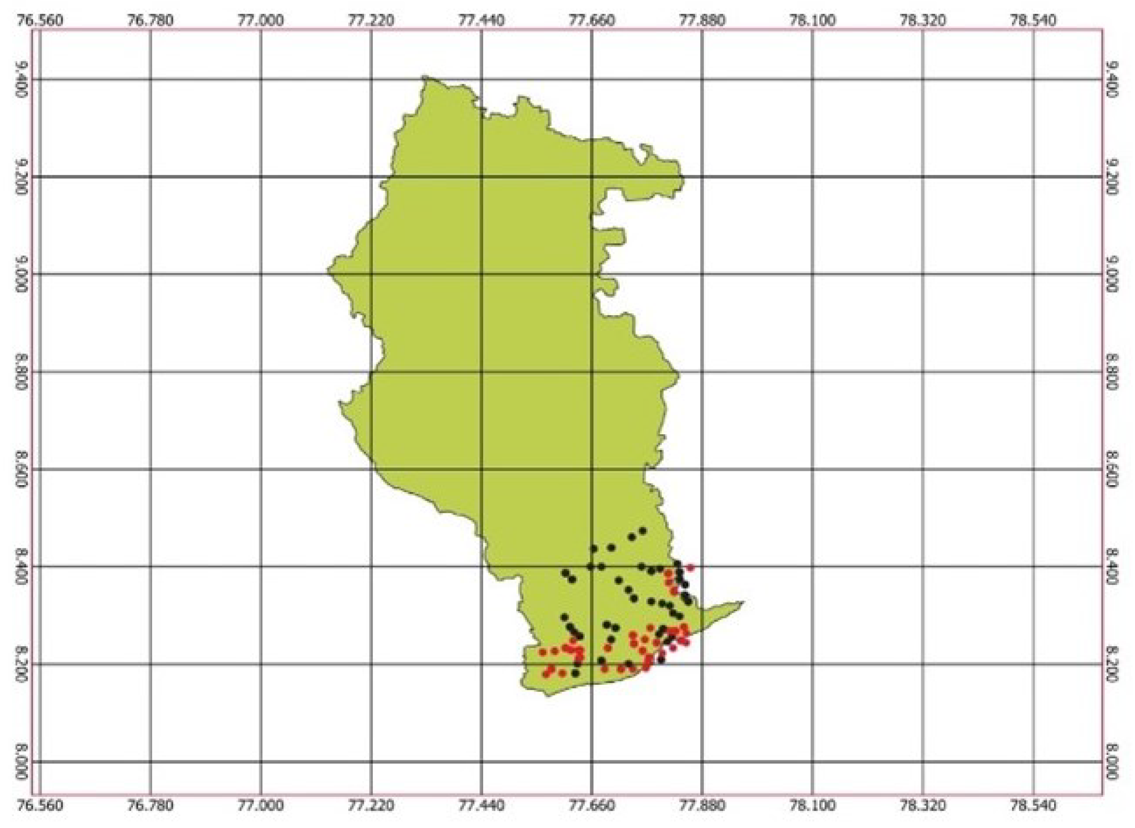
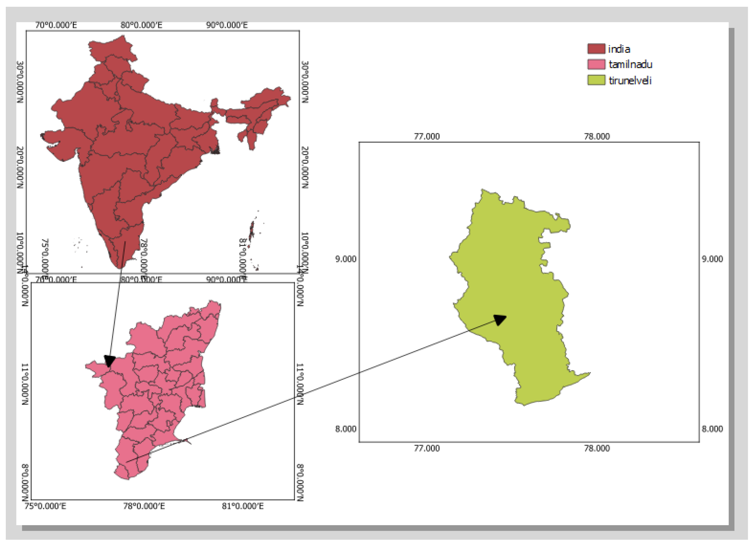
• This study aims to critically analyse the application of PRISMA hyperspectral spectroscopy in the evaluation of soil nutrient levels within the tropical region of Tamil Nadu, India.
• To generate precise and high-quality soil nutrient maps utilizing PRISMA hyperspectral data, with the aim of offering significant insights for agricultural practices, land administration, and environmental research within the specified area.
• To explore the capabilities of hyperspectral remote sensing technology in enhancing the evaluation of soil nutrient levels. This advancement has the potential to contribute to sustainable land use planning and effective crop management, particularly in tropical regions.
• In this study, we want to establish a systematic approach for utilizing hyperspectral data in order to accurately estimate essential soil nutrient parameters, specifically nitrogen, phosphorus, and potassium. Our primary emphasis will be on achieving high levels of precision and dependability in the estimation process.
• This study aims to enhance the comprehension of remote sensing techniques’ application in treating soil nutrient deficiencies and variability in tropical soils. The findings of this research can have substantial consequences for improving agricultural production and promoting sustainable land use practices in Tamil Nadu, India.

2. Materials and Methods

To verify that the spectroradiometer gets dispersed consistently, 65 soil samples were collected from Radhapuram area between 8.15 and 8.44 latitudes and between 77.64 and 77.82 longitudes, as illustrated in Figure 1. The 65 data points were divided into 45 training samples (shown as red dots in Figure 1) and 20 testing samples for model development (shown as black dots in Figure 1). Semi-micro Kjeldahl method was utilized to detect accurate organic carbon (AOC) and real nitrogen (AN) [12,13,14]. The real phosphorus and potassium contents were determined using an ultraviolet spectrophotometer, UV-2600 (made by RRSC, ISRO, Bangalore, India).

Table 1. Some soil samples of spectroradiometer data in Radhapuram, Tirunelveli District.

Sample Code	OC	N	P	K
RP-10A	0.150754	112	18.3904	272.272
RP-10B	0.150754	134.4	17.808	296.24
RP-11A	0.633166	224	51.9904	491.568
RP-11B	0.271357	168	43.1312	230.272
RP-12A	0.512563	179.2	21.4816	650.944
RP-12B	0.512563	179.2	18.48	463.344
RP-13A	0.572864	156.8	71.3328	484.176
RP-13B	0.211055	134.4	37.6992	169.344
RP-14A	0.663317	235.2	28.1456	498.288
RP-14B	0.603015	235.2	27.3168	475.888
RP-15A	0.331658	224	25.424	478.352
RP-15B	0.693467	224	36.0304	276.864
RP-16A	0.422111	156.8	17.36	474.32
RP-16B	0.723618	179.2	22.3664	520.24
RP-17A	0.874372	224	24.3264	793.408

displays spectroradiometer results for selected soil samples, calculated using techniques in Appendix A. Samples from farmers’ field were collected in coordination with Department of Agriculture using a Global Positioning System (GPS) receiver to collect geo-referenced soil samples in various locations. The collected samples were sent to the Soil Science Laboratory of CWRDM and were processed, air dried, and sieved using 2 mm sieve for further analysis. The collected soil samples were analysed for following parameters using pH, electrical conductivity (EC), organic carbon (OC), phosphorus (P), potassium (K), sulphur (S), calcium (Ca), and magnesium (Mg) using standard procedures as given in

Table A1. Standard procedures for soil chemical analysis.

Soil Properties	Method Employed
Soil pH	Potentiometric method
Electric conductivity (mmhos/cm${}^2$)	Conductivity bridge
Organic carbon (%)	Chromic acid wet digestion
Available phosphorus (kg ha${}^{-1}$)	Bray’s No.1, extractant (0.03 N ammonium fluoride + 0.025 N HCl)
Available potassium (kg ha${}^{-1}$)	NN NH4OAc extraction
Available calcium (mg kg${}^{-1}$)	NN NH4OAc versenate titration
Available magnesium (mg kg${}^{-1}$)	NN NH4OAc versenate titration
Available sulphur (mg kg${}^{-1}$)	DTPA extraction—AAS

. In addition, a model was developed to estimate the levels of nitrogen, organic carbon, phosphorus, and potassium. Figure 2 depicts the detailed flow chart of the model. The technique of our planned work is detailed in the sections that follow.

In addition, chemical characteristics and descriptive statistics of the 65 soil samples were computed and studied.

Table 2. Soil nutrient content statistics from 65 samples in Radhapuram, Tirunelveli, India.

Soil Chemical Nutrient	Dataset	Mean	Min	Max	STD	CV (%)
AOC	All	0.44	0.87	0.15	0.22	49.47
	Train	0.51	0.15	0.87	0.21	40.38
	Test	0.27	0.15	0.69	0.12	45.63
AN	All	190.23	257.60	112.00	36.69	19.29
	Train	197.46	134.40	257.60	30.72	15.56
	Test	164.08	112.00	224.00	36.21	22.07
AP	All	24.95	71.33	10.25	12.23	49.00
	Train	25.48	10.84	71.33	13.40	52.58
	Test	22.54	11.35	43.13	8.85	39.27
AK	All	437.50	1313.42	127.57	251.59	57.51
	Train	528.93	291.98	1313.42	234.98	44.42
	Test	202.08	127.57	276.86	50.66	25.07

provides statistics of soil nutrient content samples. The AOC, AN, AP, and AK content of soil varies from 0.150 g kg${}^{-1}$ to 0.874 g kg${}^{-1}$, 112 g kg${}^{-1}$ to 257.6 g kg${}^{-1}$, 10.248 g kg${}^{-1}$ to 71.332 g kg${}^{-1}$, and 127.568 g kg${}^{-1}$ to 1313.242 g kg${}^{-1}$, with mean values of 0.443, 190.22, 24.954, and 437. The coefficients of variation (CV percent) of AOC, AN, AP, and AK all fluctuated significantly [15]. According to our study area, the 65 soil samples were reasonable in terms of the diversity of soil chemical nutrients (AOC, AP, and AK).

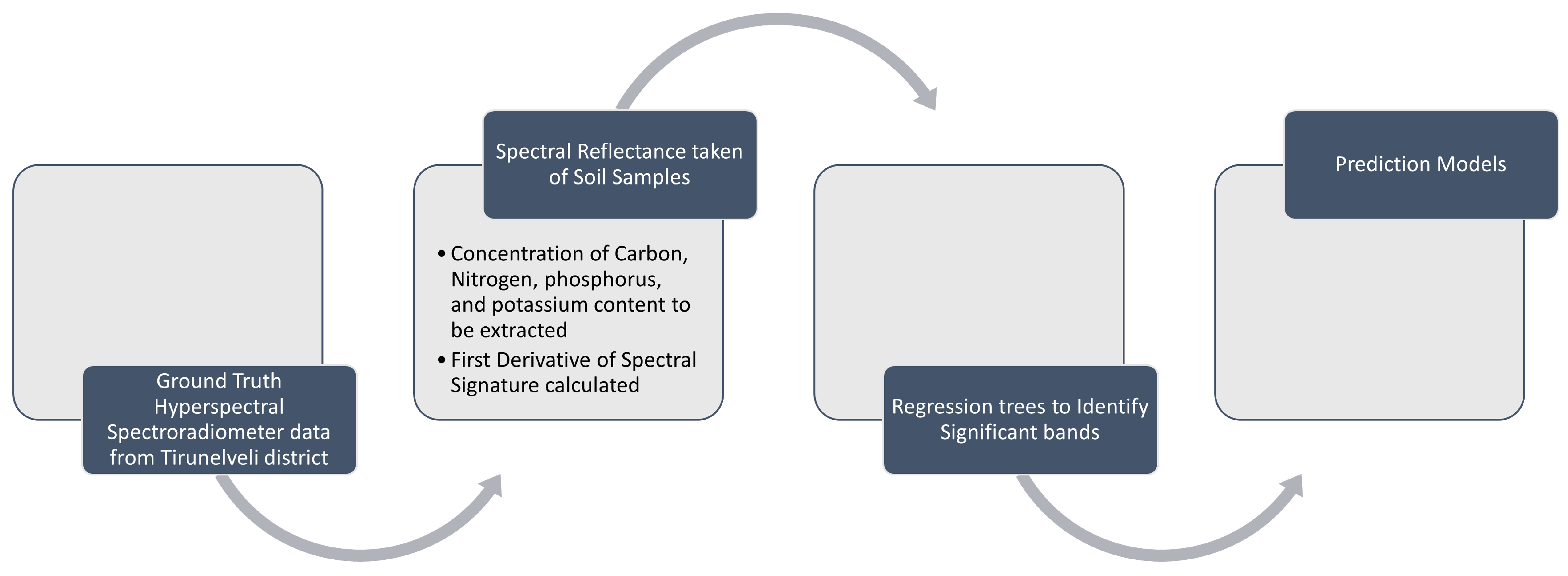
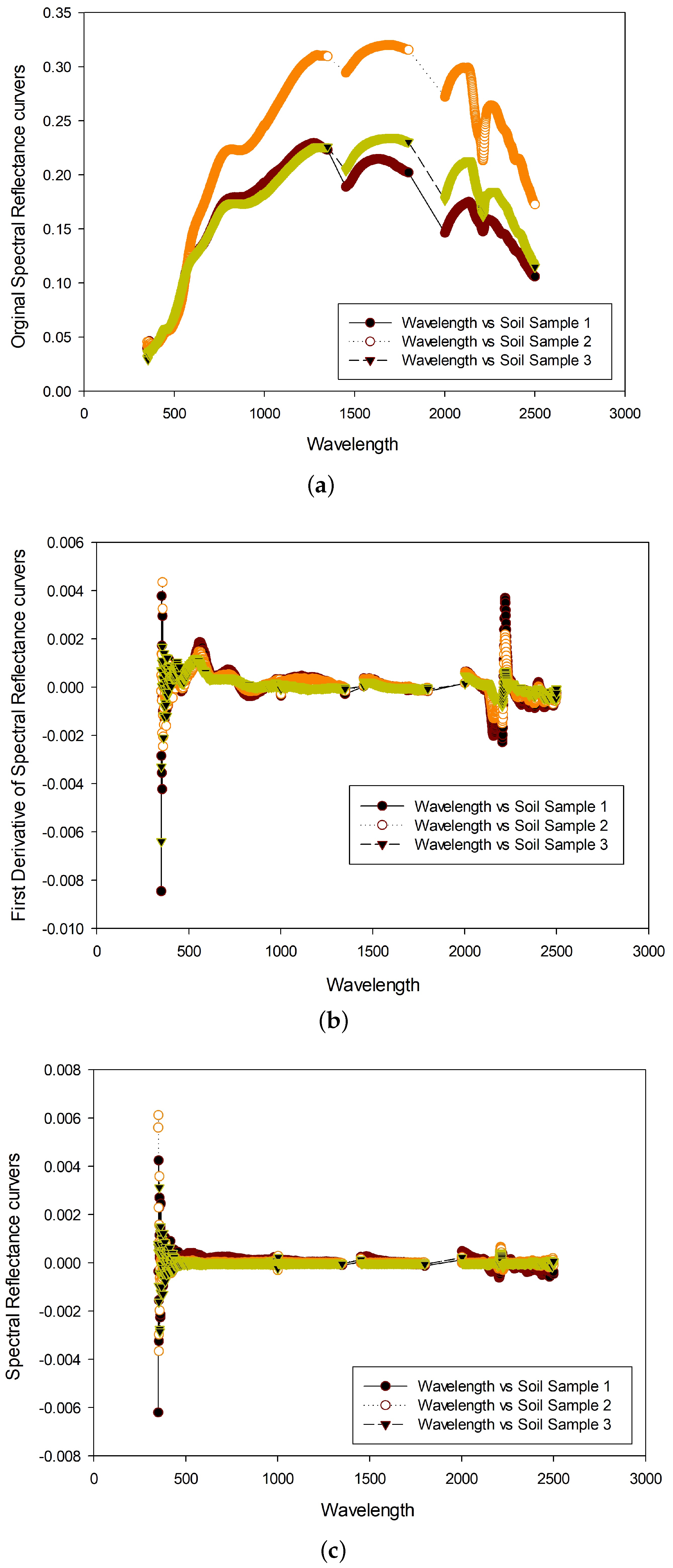
2.1. Spectral Measurement and Pre-Treatment of Soil Samples

Sixty-five soil samples were analysed in this research using a spectroradiometer with a wavelength range of 350 nm to 2500 nm at a sampling interval of 1 nm. Analytical Spectral Devices’ ASD FieldSpec4 spectroradiometer (Boulders, CO, USA) was used to collect reflectance data. Figure 3 depicts the smoothed reflectance curves of the 65 soil samples. From this plot, the soil parameters stated in the preceding section are determined.

2.2. Selection of Spectral Variables

The spectral variables and soil properties AOC, AN, AP, and AP are computed. The Pearson correction coefficient [16], one of the methods for determining the most significant p-values, is used to select the best spectral bands by studying the best coefficient. Equation (1) shows the general expression of this coefficient.

$$c_i=\frac{{\sum }_{m=1}^N({CR}_{mi}-\overline{{CR}_i})(y-\overline{y})}{\sqrt{{\sum }_{m=1}^N{(y-\overline{y})}^2}}$$

(1)

where $c_i$ is the correction coefficient between a soil nutrient (AOC, AN, AP, AK) content and a spectral reflectance variable, ${CR}_{mi}$ is the spectral reflectance of the $ith$ band of the mth soil sample, $\overline{{CR}_i}$ is the mean value of the spectral reflectance of the soil sample of the $ith$ band, and y is the spectral nutritional concentration such as AOC or AN.

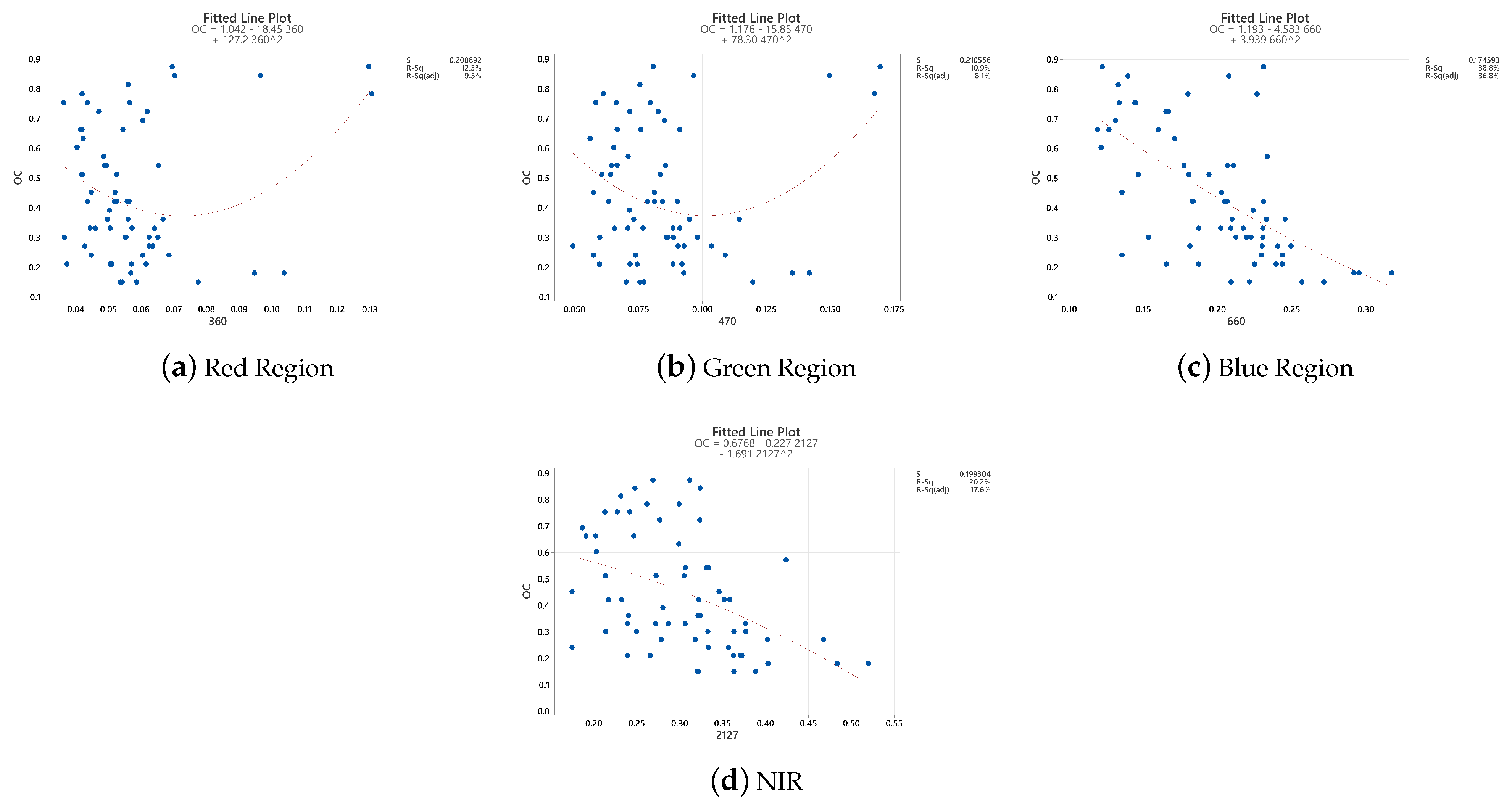
2.3. The Optimal Spectral Reflectance Variables for Soil Nutrient Concentrations

Figure 4 depicts a plot of the correlation between soil concentrations of available organic carbon (AOC), available nitrogen (AN), available phosphorus (AP), and available potassium (AK), and spectral indices of raw soil reflectance, first derivative (FD), and second derivative (SD) [17,18,19].

Table 3. The best spectral variables to predict four soil nutrients.

Soil Nutrient	Selected Spectral Variables	Pearson Correlation Coefficients
AOC	R353, R1640, FD642, FD1676, SD392, SD1245	−0.34 **, 0.26 **, 0.47 **, 0.35 **, 0.34 **, −0.26 **
AN	R1256, FD796, FD1122, FD2132, SD556	−0.23 **, 0.25 **,0.36 **, 0.45 **, 0.43 **
AP	R2245, R2486, FD1545, FD1702, SD657	0.14 **, 0.50 **, 0.45 **, −0.26 **, 0.32 **
AK	R1498, FD542, SD1635, SD2456	0.24 **, 0.47 **, −0.36 **, 0.33 **, 0.28 **

** Indicates significant correlation at (p < 0.01) level.

depicts spectral reflectance variables based on significance values less than 0.01.

2.4. Calculation and Evaluation of Soil Nutrient Concentrations at Soil Reflectance Locations with Precision

The spectral parameters chosen for this study served as independent variables. As shown in

Table 4. Regression tree predictions for AOC, AN, AP, and AK values.

	Datasets	R-Squared (R2)	Root Mean Squared Error (RMSE)	Mean Squared Error (MSE)	Mean Absolute Percent Error (MAPE)
AOC	Train	100.00%	0	0	0
	Test	97.50%	0.124	0.0154	0.04
AN	Train	99.99%	0.0005	0	0.0026
	Test	99.98%	0.0007	0	0.0039
AP	Train	51.02%	8.4924	72.1203	0.2286
	Test	49.93%	8.5864	73.7256	0.2294
AK	Train	26.72%	213.7068	45,670.578	0.3795
	Test	25.06%	216.123	46,709.154	0.3865

, soil nutrient characteristics AOC, AN, AP, and AK were used as dependent variables. The PLSR’s goal is to forecast the contents of soil AOC, AN, and sub-1640 AK. Between the expected and actual concentrations, the relative root mean square error (RRMSE) and coefficient of determination (R2) are calculated [18,19]. Equations (2)–(5) are used to calculate the obtained PLSR estimation.

$$TOC=0.714+R_{453}\ast 0.214-R_{1640}\ast 24.32+{FD}_{642}\ast 184.24-{SD}_{492}\ast 19.22-{SD}_{1245}\ast 124.26$$

(2)

$$TN=0.227+R_{1256}\ast 0.635-{FD}_{796}\ast 124.87+{FD}_{1122}\ast 241.18-{FD}_{2132}\ast 0.92-{SD}_{556}\ast 234.26$$

(3)

$$TP=0.912-R_{2245}\ast 0.174+R_{2486}\ast 0.24+{FD}_{1545}\ast 122.46+{FD}_{1702}\ast 113.2-{SD}_{657}\ast 218.26$$

(4)

$$TK=0.523-R_{1498}\ast 0.637-{FD}_{635}\ast 17.87-{SD}_{1635}\ast 247.24+{SD}_{2456}\ast 98.67$$

(5)

Table 4 shows the regression tree’s prediction error rate for AOC, AN, AP, and AK. AOC gives better performance than other chemical properties. AOC values help to identify more bands in our proposed work. In the case of AOC having a 0.9750 R2 value, an RMSE of 0.124 was obtained for the test dataset. These four chemical properties are shown in Table 4.

3. Results and Discussion

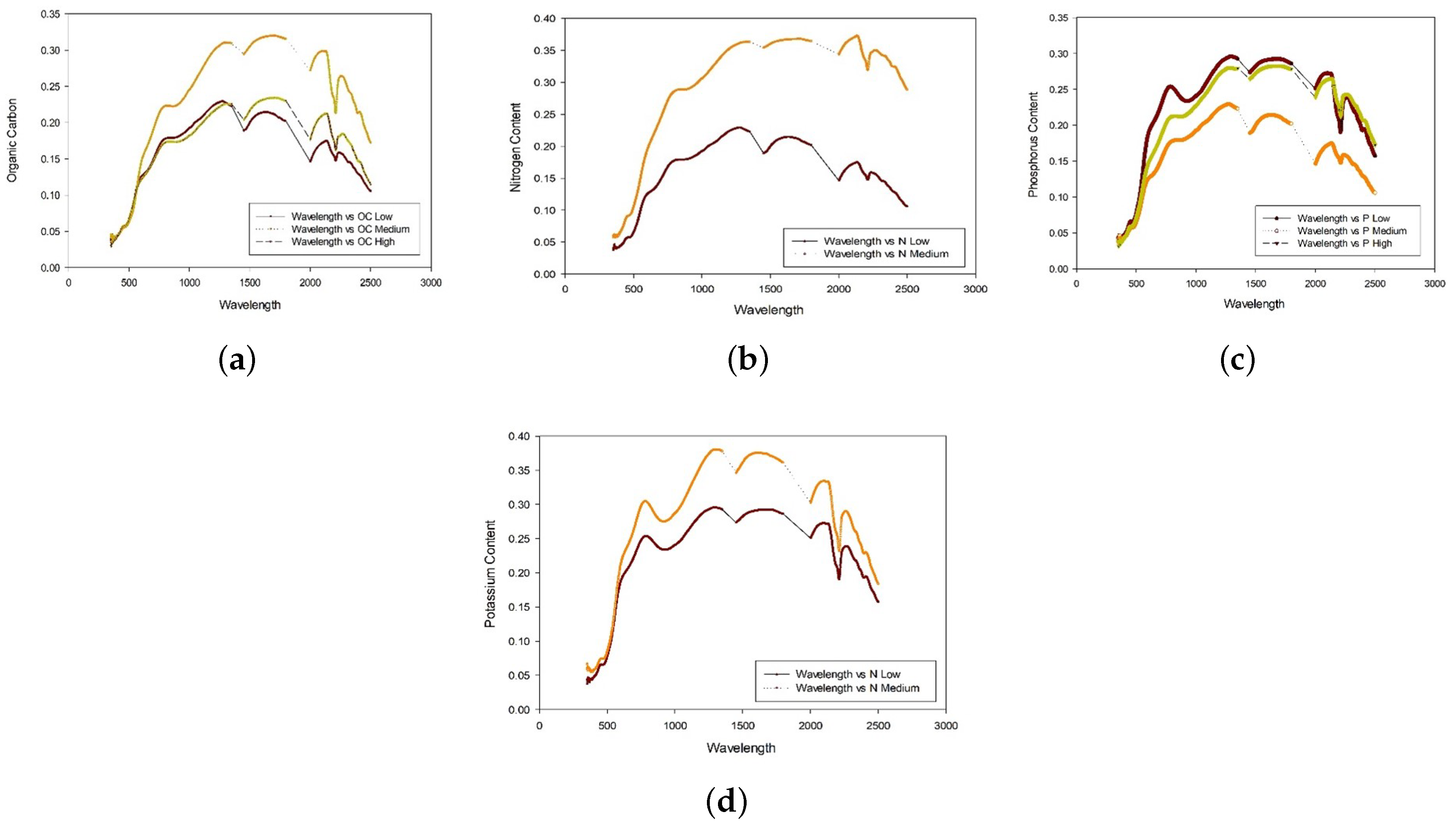
3.1. AOC Concentration in Radhapuram, Tirunelveli District

In this research, the selected spectral variables were used as independent variables, while the soil chemical nutrients (AOC, AN, AP, and AK) were used as dependent variables [20,21]. The correlation coefficient and relative root mean square error were used to assess the accuracy of the estimation models by approximating the soil AOC, AN, AP, and AK contents. The mean absolute deviation and present fundamental error were calculated for the training and testing datasets.

Table 5. Comparison of proposed work with PSO, GAO, and CSO.

Optimization Algorithms	Running Time	Important Parameter Involved	Convergence for Hyperspectral Band Selection	Iteration for Obtaining Global Minimum	Accuracy for Selecting Optimal Relevant Hyperspectral Bands
PSO [5]	Low	Learning factor, number of dimensions, range of particles, Vmax max change of particle velocity	Moderate	1100	High
GWO [5]	Moderate	Population size, mutation, and crossover probability	Slow	450	Moderate
CSO [5]	High	Number of nests, Levy flight solution	Fast	400	Moderate
FPO [5]	Very High	Number of flowers	Very Fast	150	Very High

shows the importance of different optimization techniques used and compares the same.

As represented in Table 5, the soil nutrient predictions were carried out using different bands including visible bands, near-infrared bands, VNIR+NIR region bands, and bands developed using 150 random bands [22,23]. The AOC, AN, AP, and AK contents of the soil were predicted and the PLSR model was validated.

Table 6. AOC prediction for different bands for the PLSR prediction model with different optimization techniques.

Optimization Techniques	RMSE	R-Squared	MSE	MAE
PSO	0.152	0.890	0.023	0.124
CSO	0.136	0.910	0.019	0.116
GWO	0.154	0.870	0.024	0.129
MFO	0.106	0.840	0.011	0.086
Hybrid Optimization	0.182	0.970	0.033	0.157

shows the AOC prediction for different bands for the PLSR prediction model [22,24].

The results show the best performance using the PLSR methods and VNIR+NIR regions because R2 is 0.970, as shown in Figure 5.

In the proposed method, the regression trees divide the data into different groups. As shown in Equation (6), the algorithm divides the space using rectangles to make the data easier to read and to find boxes that reduce the RSS (residual sum of squares).

$$Regression=\sum _{j=1}^J\sum _{i=R^j}{(y_i-{\widehat{y}}_{R_j})}^2$$

(6)

The partitioning of the feature space into j boxes was not computationally feasible. This is addressed using recursive binary splinting, a top-down greedy technique. The top-down approach, which begins at the top of the tree, divides the predictor space into two new branches at each stage, as illustrated in Figure 6. AOC is divided into three levels based on spectral reflectance, whereas AN, AP, and AK are divided into two. AOC seems to have a mean of 0.8307 and a standard deviation (STD) of 0.3749 from 65 soil samples, which will be divided into two levels based on the threshold value of 151.2. If the nitrogen content is less than 151.2, it is mapped to a low value and, if it is greater than 151.2, it is mapped to a medium value which is shown in Figure 6.

In the case of AOC, the mean is 0.5692 and the standard deviation is 0.7838. These three levels are separated by a threshold value of 0.4824. If the organic carbon content is less than 0.4824, it is classified as low. Otherwise, it is assigned to a different category. These categories are classified into two levels: medium and high. If the organic carbon value is less than 0.708453, it is assigned to medium weights while the other is assigned to high weights. Out of 65 samples, 40 are low value, 13 are medium value, and the remaining 12 are high value. In terms of phosphorus, the mean of 65 soil samples is 24.954 and the standard deviation is 12.134 [25,26]. AP is divided into two levels, which are distinguished by their phosphorus content. If the phosphorus value is less than 1.5, it is assigned a low value; otherwise, it is assigned a high value. In terms of potassium, the mean of 65 soil samples is 437.500 and the standard deviation is 249.650. AK is classified into two levels based on its potassium content [27,28]. If the potassium value is less than 1.5, it is assigned a low value; otherwise, it is assigned a high value. Figure 7 depicts the classification of AOC, AN, AP, and AK.

The PLSR approach for soil spectroscopic analysis was evaluated using hyperspectral data from soil samples obtained in a laboratory, to estimate the amounts of the soil nutrients AOC, AN, AP, and AK. The soil nutrients could be predicted using RGB bands, near-infrared, individual RGB, and the VNIR+NIR region, according to the results [29,30]. The PLSR method performed best for combined VNIR+NIR regions, with an R2 value of 0.970, indicating that nutrients can be better predicted, and the PRISMA hyperspectral images were also used to evaluate lab-driven models in the area to increase soil nutrient content on a regional scale. PLSR approaches indicate the RMSE values for all the soil nutrients in the validation datasets and AOC has the best impact on HSI images.

3.2. Estimation of Soil Nutrient Content for Satellite PRISMA Hyperspectral Region

PRISMA (Precursors IperSpettrale Della Mission Applicative) is an Italian hyperspectral imaging spacecraft that was launched in 2023 [31]. This space-borne mission collects data from three different spectral regions: the very near infrared region (VNIR), the short wave infrared region (SWIR), and the panchromatic region (PR). The VNIR spectrum spans 400 nm to 1010 nm, with a spectral resolution of 12 nm, 66 continuous spectrum bands, and a spatial resolution of 30 m [32,33]. In SWIR, the spectrum ranges from 920 nm to 2505 nm with 12 nm spectral resolution, 171 endless spectrum bands, and 30 m spatial resolution. The spectrum ranges from 400 nm to 700 nm in PR with a one-micrometer spectrum band and 5 m spatial resolution, as shown in

Table 7. Dataset descriptions forPRISMA data.

Product Name	PRS_L2D_STD_20201211052010_ 20201211052014_0001.HE5	Product Id	PRS_L2D_STD
Processor Version	02.04	L1 Processor Version	-
Processor Name	L2D	Processing Time	2021-08-11T04:56:29.000749
Processing Level	2D	Acquisition Type	EARTH OBSERVATION
Acquisition Size	30 KM	Acquisition Purpose	NOT SPECIAL PRODUCT
Number of Bands (VNIR + SWIR)	234	Image Id	15549
Product Start Time	2020-12-11T05:20:10.524999	Product Stop Time	2020-12-11T05:20:14.830690
Sun Zenith Angle	39.602°	View Zenith Angle	15.724°

.

3.3. Methodology

3.3.1. Preprocessing Levels of PRISMA Hyperspectral Data

Figure 8 shows the conversion of three different levels of PRISMA data [34].

• Level 0: the raw binary files, comprising instrument data and cloud percentage, are included in the L0 data product.
• Level 1: the L1 data product contains radiometrically calibrated data for hyperspectral and panchromatic radiance cubes on the top of the atmospheric radiance image.
• Level 2: the L2 data product is further split into three different groups:

  -

  L2B: atmospheric calibration and geolocation of the L1 data product, i.e., atmospheric radiance at the bottom.

  -

  L2C: atmospheric calibration and geolocation of the L1 data product, i.e., bottom of atmospheric radiance including aerosol thickness and map of water vapour.

  -

  L2D: orthorectification of L2C with significantly less cloud coverage.

• Level 1 and Level 2 data are generated in the Hierarchical Data format release 5 (HDF5 or he5). In this work, we have used Level2D data to identify paddy production in a particular area.

3.3.2. File Format Conversion

Data in L2D is available in HDF5 or hex cube format. The he5 format has been converted to tiff or hdr format in accordance with the specifications. The open-source software R programming is extremely beneficial in restoring the same. To complete the data format conversion, the following steps must be taken. (1). The pr_convert function is used to import PRISMA L2 data (2B, 2C, and 2D). The pr convert function is used to import PRISMA L2 data (2B, 2C, 2D). It takes a PRISMA L1 hdf5 image as input, as well as the name and format of an output folder, and has a series of switches for selecting which hyperspectral cubes and auxiliary datasets to generate. (2). In VNIR and SWIR, the logical justifications for and against importing VNIR and SWIR hyperspectral cubes are presented. (3). The full logical argument can be used to determine whether a full VNIR+SWIR cube is required.

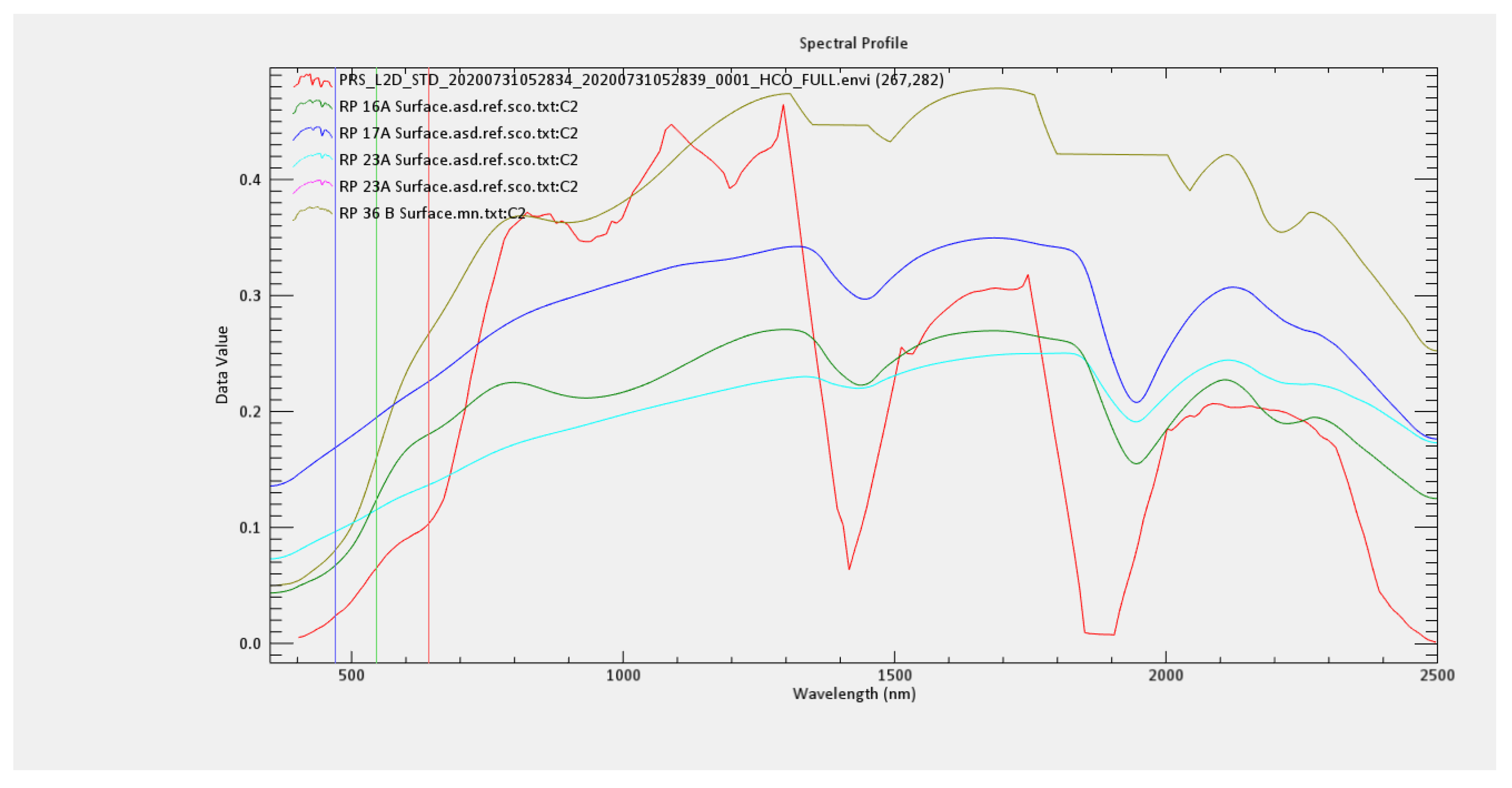
3.3.3. PRISMA Dataset Descriptions

Figure 9 depicts the location of the study in India (11°38′ N, 78°10′ E) with a land coverage of 900 km${}^2$. The study area is in the Tirunelveli District, Tamil Nadu, India and the most comprehensive soil mapping provides less than 0.4 percent cloud coverage. From 402 to 2500 nm, a total of 143 bands are present. As illustrated in Figure 9, the SAM classification identifies the amount of soil that matches the original spectra. The 4th, 17th, 18th, and 63rd Digital Numbers (DNs) of 65 soil samples have the best mapping with more AOC content. The fourth reflectance soil sample had 662,569 points and a success rate of 47.24 percent [35,36]. Table 6 shows the number of points for the remaining soil samples.

Four lab-derived models were used to map the soil nutrient levels (AOC, AN, AP, and AK) for the study area at the regional scale using the ideal spectral characteristics from the PRISMA image. By resampling the PRISMA spectral data to predict soil nutrient concentrations, the original ideal spectral variables for AOC, AN, AP, and AK were obtained. Figure 10 shows that the PLSR indicated soil nutrient concentration is the best match spectra based on laboratory hyperspectral data. Using linear spectral unmixing analysis, the ideal spectral variables for soil components were generated from the bands. When applied to PLSR, lab-derived models with optimal spectral variables produced better results, but PLSR produced similar regional distributions of soil nutrient concentrations.

The PRISMA HSI data are also used to map soil nutrient levels in the study area in order to test the PLSR prediction models’ regional scale applicability. Figure 11 shows that the AOC content was more reliable than the AN, AP, and AK contents, indicating that the SAM could map soil AOC content at the regional scale using PRISMA HSI images which is shown in Figure 11. SAM models are used to map soil AOC content. Soil nutrient content prediction accuracy using the PRISMA HSI image was only moderately better than measured hyperspectral data due to differences in spectral band ranges between measured hyperspectral data and hyperspectral images. These variables will be taken into account in future analyses. PRISMA and ground truth data were used for the spectral mapping. SAM performs comparably with other per-pixel-based classification systems in terms of classification results [37,38,39]. The SAM approach analyses images and soil spectra, and manipulates the angular distance between the image and soil spectra. In total, 173 bands are present from 402 to 2500 nm [40,41]. The SAM classification identifies the amount of soil that matches with the original spectra, as shown in Figure 10. Out of 65 soil samples, the 4th, 17th, 18th, and 63rd Digital Numbers (DN) are the samples that have the best mapping with more AOC content [15,31,34]. The fourth reflectance soil sample had 662,569 points at 47.24%. The numbers of points for the remaining soil samples are shown in

Table 8. Mapping of raw spectral reflectance with PRISMA hyperspectral data.

DN Reflectance Soil Sample	Number of Points	Actual	Percentage Accuracy
RP16A	662,577	662,577	47.2648
RP17A	589,432	1,252,009	89.3118
RP23A	149,615	1,401,624	99.9846
RP36B	5	1,401,629	99.9849
RP8A	207	1,401,836	99.9997
RP98	4	1,401,840	100.0000

.

4. Conclusions

The PLSR approach for soil spectroscopic analysis was evaluated using hyperspectral data from soil samples obtained in a laboratory in Radhapuram, India, to estimate the amounts of the soil nutrients AOC, AN, AP, and AK. The soil nutrients could be predicted using RGB bands, near-infrared, individual RGB, and the VR+NIR region, according to the results. The PLSR method performed best for the combined VR+NIR regions, with an R2 value of 0.970, indicating that nutrients could be better predicted. PRISMA hyperspectral images were also used to evaluate lab-driven models in Radhapuram’s Tirunelveli district to increase soil nutrient content on a regional scale. The RMSE values for all soil nutrients in the validation datasets are indicated by PLSR approaches and AOC has the greatest impact on HIS images. As a result, spectral prediction models could be improved, and soil nutrient content could be predicted more accurately using PRISMA hyperspectral images. The research findings provided an important reference for the high-accuracy prediction of soil nutrients.

References

1. Nocita, M.; Stevens, A.; Van Wesemael, B.; Aitkenhead, M.; Bachmann, M.; Barthès, B.; Dor, E.B.; Brown, D.J.; Clairotte, M.; Wetterlind, J.; et al. Soil spectroscopy: An alternative to wet chemistry for soil monitoring. Adv. Agron. 2015, 132, 139–159. [Google Scholar]
2. Stenberg, B.; Rossel, R.A.V.; Mouazen, A.M.; Wetterlind, J. Visible and near-infrared spectroscopy in soil science. Adv. Agron. 2010, 107, 163–215. [Google Scholar]
3. Ben-Dor, E.; Chabrillat, S.; Demattê, J.A.M.; Taylor, G.R.; Hill, J.; Whiting, M.L.; Sommer, S. Using imaging spectroscopy to study soil properties. Remote Sens. Environ. 2009, 113, S38–S55. [Google Scholar] [CrossRef]
4. Hively, W.D.; McCarty, G.W.; Reeves, J.B.; Lang, M.W.; Oesterling, R.A.; Delwiche, S.R. Use of airborne hyperspectral imagery to map soil properties in tilled agricultural fields. Appl. Environ. Soil Sci. 2011, 2011, 358193. [Google Scholar] [CrossRef]
5. Parikh, S.J.; Goyne, K.W.; Margenot, A.J.; Mukome, F.N.; Calderón, F.J. Soil chemical insights provided through vibrational spectroscopy. Adv. Agron. 2014, 126, 1–148. [Google Scholar]
6. An, R.; Samiaappan, S.; Veni, S.; Worch, E.; Zhou, M. Airborne hyperspectral imagery for band selection using moth–flame metaheuristic optimization. J. Imaging 2022, 8, 126. [Google Scholar]
7. Gao, H.Z.; Lu, Q.P. Near infrared spectral analysis and measuring system for primary nutrient of soil. Spectrosc. Spectr. Anal. 2011, 31, 1245–1249. [Google Scholar]
8. Leone, A.P.; Viscarra-Rossel, R.A.; Amenta, P.; Buondonno, A. Prediction of soil properties with PLSR and vis-NIR spectroscopy: Application to mediterranean soils from Southern Italy. Curr. Anal. Chem. 2012, 8, 283–299. [Google Scholar] [CrossRef]
9. Ramoelo, A.; Skidmore, A.K.; Cho, M.A.; Mathieu, R.; Heitkönig, I.M.A.; Dudeni-Tlhone, N.; Schlerf, M.; Prins, H.H.T. Nonlinear partial least square regression increases the estimation accuracy of grass nitrogen and phosphorus using in situ hyperspectral and environmental data. ISPRS J. Photogramm. Remote Sens. 2013, 82, 27–40. [Google Scholar] [CrossRef]
10. Balabin, R.M.; Lomakina, E.I. Support vector machine regression (SVR/LS-SVM)—An alternative to neural networks (ANN) for analytical chemistry? Comparison of nonlinear methods on near infrared (NIR) spectroscopy data. Analyst 2011, 136, 1703–1712. [Google Scholar] [CrossRef]
11. Balabin, R.M.; Smirnov, S.V. Interpolation and extrapolation problems of multivariate regression in analytical chemistry: Benchmarking the robusANess on near-infrared (NIR) spectroscopy data. Analyst 2012, 137, 1604–1610. [Google Scholar] [CrossRef] [PubMed]
12. Li, D. Estimating the blood glucose of serum optical spectrum using support vector regression. In Proceedings of the Fourth International Conference on Photonics and Optical Engineering, Xi’an, China, 15–16 October 2020; International Society for Optics and Photonics: Bellingham, WA, USA, 2021; Volume 11761, p. 117611U. [Google Scholar]
13. Walkley, A. An Examination of Methods for Determining Organic Carbon and Nitrogen in Soils1. (with One Text-figure). J. Agric. Sci. 1935, 25, 598–609. [Google Scholar] [CrossRef]
14. Peng, Y.; Zhao, L.; Hu, Y.; Wang, G.; Wang, L.; Liu, Z. Prediction of soil nutrient contents using visible and near-infrared reflectance spectroscopy. ISPRS Int. J. Geo-Inf. 2019, 8, 437. [Google Scholar] [CrossRef]
15. Yao, L.; Xu, M.; Liu, Y.; Niu, R.; Wu, X.; Song, Y. Estimating of heavy metal concentration in agricultural soils from hyperspectral satellite sensor imagery: Considering the sources and migration pathways of pollutants. Ecol. Indic. 2024, 158, 111416. [Google Scholar] [CrossRef]
16. Morrissey, M.B.; Ruxton, G.D. Multiple regression is not multiple regressions: The meaning of multiple regression and the non-problem of collinearity. Philos. Theory Pract. Biol. 2018, 10, 3. [Google Scholar] [CrossRef]
17. Ren, H.-Y.; Zhuang, D.F.; Singh, A.N.; Pan, J.-J.; Qiu, D.-S.; Shi, R.-H. Estimation of As and Cu contamination in agricultural soils around a mining area by reflectance spectroscopy: A case study. Pedosphere 2009, 19, 719–726. [Google Scholar]
18. Wang, F.; Wang, F.; Zhang, Y.; Hu, J.; Huang, J.; Xie, J. Rice yield estimation using parcel-level relative spectral variables from UAV-based hyperspectral imagery. Front. Plant Sci. 2019, 10, 453. [Google Scholar] [CrossRef]
19. Yaseen, Z.M.; Tran, M.T.; Kim, S.; Bakhshpoori, T.; Deo, R.C. Shear strength prediction of steel fiber reinforced concrete beam using hybrid intelligence models: A new approach. Eng. Struct. 2018, 177, 244–255. [Google Scholar] [CrossRef]
20. Singh, S.; Sarma, K. Exploring Soil Spatial Variability with GIS, Remote Sensing, and Geostatistical Approach. J. Soil Plant Environ. 2023, 2, 79–99. [Google Scholar] [CrossRef]
21. Loizzo, R.; Guarini, R.; Longo, F.; Scopa, T.; Formaro, R.; Facchinetti, C.; Varacalli, G. PRISMA: The Italian hyperspectral mission. In Proceedings of the IGARSS 2018–2018 IEEE International Geoscience and Remote Sensing Symposium, Valencia, Spain, 22–27 July 2018; pp. 175–178. [Google Scholar]
22. Folkman, M.A.; Pearlman, J.; Liao, L.B.; Jarecke, P.J. EO-1/Hyperion hyperspectral imager design, development, characterization, and calibration. Hyperspectral Remote Sens. Land Atmos. 2001, 4151, 40–51. [Google Scholar]
23. Hecker, C.; Van der Meijde, M.; van der Werff, H.; van der Meer, F.D. Assessing the influence of reference spectra on synthetic SAM classification results. IEEE Trans. Geosci. Remote Sens. 2018, 46, 4162–4172. [Google Scholar] [CrossRef]
24. Guarini, R.; Loizzo, R.; Facchinetti, C.; Longo, F.; Ponticelli, B.; Faraci, M.; Di Nicolantonio, W. PRISMA hyperspectral mission products. In Proceedings of the IGARSS 2018–2018 IEEE International Geoscience and Remote Sensing Symposium, Valencia, Spain, 22–27 July 2018; pp. 179–182. [Google Scholar]
25. Christian, B.; Krishnayya, N.S.R. Classification of tropical trees growing in a sanctuary using Hyperion (EO-1) and SAM algorithm. Curr. Sci. 2009, 96, 1601–1607. [Google Scholar]
26. Zhang, X.; Li, P. Lithological mapping from hyperspectral data by improved use of spectral angle mapper. Int. J. Appl. Earth Obs. Geoinf. 2014, 31, 95–109. [Google Scholar] [CrossRef]
27. Harris, A.T. Spectral mapping tools from the earth sciences applied to spectral microscopy data. Cytom. Part A J. Int. Soc. Anal. Cytol. 2006, 69, 872–879. [Google Scholar] [CrossRef] [PubMed]
28. An, R.; Veni, S.; Aravinth, J. Robust classification technique for hyperspectral images based on 3D-discrete wavelet transform. Remote Sens. 2021, 13, 1255. [Google Scholar]
29. An, R.; Veni, S.; Geetha, P.; Subramoniam, S.R. Extended morphological profiles analysis of airborne hyperspectral image classification using machine learning algorithms. Int. J. Intell. Networks 2021, 2, 1–6. [Google Scholar]
30. Aravinth, J.; Nath, B.; Subramanian, M.S.; Bulusu, R.V.; Monish, P. Machine learning based Detection of Zinc Mineralization North India using Hyperspectral Image Processing. In Proceedings of the 2019 International Conference on Communication and Electronics Systems (ICCES), Coimbatore, India, 17–19 July 2019; pp. 1777–1781. [Google Scholar]
31. Zhong, L.; Yang, S.; Chu, X.; Sun, Z.; Li, J. Inversion of heavy metal copper content in soil-wheat systems using hyperspectral techniques and enrichment characteristics. Sci. Total. Environ. 2024, 907, 168104. [Google Scholar] [CrossRef]
32. Mohan, D.; Aravinth, J.; Rajendran, S. Reconstruction of Compressed Hyperspectral Image Using SqueezeNet Coupled Dense Attentional Net. Remote Sens. 2023, 15, 2734. [Google Scholar] [CrossRef]
33. Shanthi, T.; An, R.; Annapoorani, S.; Birundha, N. Analysis of Phonocardiogram Signal Using Deep Learning. In International Conference on Innovative Computing and Communications; Springer: Singapore, 2023; pp. 621–629. [Google Scholar]
34. Pan, B.; Cai, S.; Zhao, M.; Cheng, H.; Yu, H.; Du, S.; Xie, F. Predicting the Surface Soil Texture of Cultivated Land via Hyperspectral Remote Sensing and Machine Learning: A Case Study in Jianghuai Hilly Area. Appl. Sci. 2023, 13, 9321. [Google Scholar] [CrossRef]
35. Lawrence, R.; Labus, M. Early detection of Douglas-fir beetle infestation with subcanopy resolution hyperspectral imagery. West. J. Appl. For. 2003, 18, 202–206. [Google Scholar] [CrossRef]
36. Golia, E.E.; Diakoloukas, V. Soil parameters affecting the levels of potentially harmful metals in Thessaly area, Greece: A robust quadratic regression approach of soil pollution prediction. Environ. Sci. Pollut. Res. 2022, 29, 29544–29561. [Google Scholar] [CrossRef] [PubMed]
37. Ashokkumar, S.R.; Anupallavi, S.; Premkumar, M.; Jeevanantham, V. Implementation of deep neural networks for classifying electroencephalogram signal using fractional S-transform for epileptic seizure detection. Int. J. Imaging Syst. Technol. 2021, 31, 895–908. [Google Scholar] [CrossRef]
38. Bowker, D.E. Spectral Reflectances of Natural Targets for Use in Remote Sensing Studies; NASA: Washington, DC, USA, 1985; Volume 1139.
39. Benesty, J.; Chen, J.; Huang, Y.; Cohen, I. Pearson correlation coefficient. In Noise Reduction in Speech Processing; Springer: Berlin/Heidelberg, Germany, 2009; pp. 1–4. [Google Scholar]
40. Tsai, F.; Philpot, W. Derivative analysis of hyperspectral data. Remote Sens. Environ. 1998, 66, 41–51. [Google Scholar] [CrossRef]
41. Guo, L.; Zhang, H.; Shi, T.; Chen, Y.; Jiang, Q.; Linderman, M. Prediction of soil organic carbon sAOCk by laboratory spectral data and airborne hyperspectral images. Geoderma 2019, 337, 32–41. [Google Scholar] [CrossRef]
Figure 1. Flow chart of soil content mapping with hybrid optimizations.
Applsci 14 00186 g001
Figure 2. Flow chart of band selection in soil data.
Applsci 14 00186 g002
Figure 3. Spectral reflectance of 65 different soil samples.
Applsci 14 00186 g003
Figure 4. Pearson correlation coefficients between soil concentration contents and three soil spectral reflectances: (a) raw spectral reflectance of three soil samples; (b) first derivative; and (c) the second derivative.
Applsci 14 00186 g004
Figure 5. Prediction of AOC for different band selections.
Applsci 14 00186 g005
Figure 6. Prediction of AOC for different band selections. (a) AOC split into three different levels (low, medium, high). (b) AN split into two different levels (low, medium). (c) AP split into two different levels (low, medium). (d) AK split into two different levels (low, medium).
Applsci 14 00186 g006
Figure 7. Spectral reflectance for different AOC, AN, AP, and AK levels. (a) Spectral reflectance curves for three AOCs. (b) Spectral reflectance curves for two ANs. (c) Spectral reflectance curves for three APs. (d) Spectral reflectance curves for two AKs.
Applsci 14 00186 g007
Figure 8. Mapping ground truth raw soil data with PRISMA hyperspectral data.
Applsci 14 00186 g008
Figure 9. Study area for soil mappingin Tirunelveli district, Tamilnadu, India.
Applsci 14 00186 g009
Figure 10. Spectral mapping with PRISMA and ground truth data.
Applsci 14 00186 g010
Figure 11. Spectral mapping with PRISMA and ground truth data using SAM classifier.
Applsci 14 00186 g011