Article

Estimating Riparian Vegetation Volume in the River by 3D Point Cloud from UAV Imagery and Alpha Shape

Department of Hydro Science and Engineering Research, Korea Institute of Civil Engineering and Building Technology (KICT), Goyang-si 10223, Republic of Korea
*
Author to whom correspondence should be addressed.
Appl. Sci. 2024, 14(1), 20; https://doi.org/10.3390/app14010020
Submission received: 10 November 2023 / Revised: 15 December 2023 / Accepted: 18 December 2023 / Published: 19 December 2023
(This article belongs to the Special Issue Navigation and Object Recognition with 3D Point Clouds)

Abstract

:
This study employs technology that has many different applications, including flood management, flood level control, and identification of vegetation type by patch size. Recent climate change, characterized by severe droughts and floods, intensifies riparian vegetation growth, demanding accurate environmental data. Traditional methods for analyzing vegetation in rivers involve on-site measurements or estimating the growth phase of the vegetation; however, these methods have limitations. Unmanned aerial vehicles (UAVs) and ground laser scanning, meanwhile, offer cost-effective, versatile solutions. This study uses UAVs to generate 3D riparian vegetation point clouds, employing the alpha shape technique. Performance was evaluated by analyzing the estimated volume results, considering the influence of the alpha radius. Results are most significant with an alpha radius of 0.75. This technology benefits river management by addressing vegetation volume, scale, flood control, and identification of vegetation type.

1. Introduction

Due to recent global climate change, a noticeable increase in riparian vegetation is evident, regardless of the river’s size and location or the presence of structures [1,2,3,4,5]. In one study [4], the expansion of the vegetation area was analyzed using aerial photo analysis, and the results showed that vegetation in Cheongmi Stream and Seomgang had increased by about two times since 2010, and in Naeseong Stream vegetation had increased by about 17 times in the same time period. This change resulted in a decrease in sandbanks and water surface area. Even without the impact of climate change, rivers continuously evolve with the creation, decline, and movement of riverbanks; nonetheless, the increase in vegetation in river environments is undeniable [3,4,5,6,7,8]. Woo et al. [9,10] suggested that the causes of vegetation translocation in rivers include the use of dams to suppress spring floods and reduce summer floods, changes in rainfall patterns, artificial disturbance of river channels, and an increased influx of nutrients into rivers. This increase in riparian vegetation can cause various problems, such as a rapid rise in water levels during floods and transitions in terrestrial ecosystems [9]. Additionally, long-term vegetation adhesion affects sediment accumulation and flow reduction, leading to raised riverbeds [11]. Therefore, to manage the changing river environment, there is a demand for technology that can precisely determine the river’s physical shape and vegetation adhesion status. Until now, aquatic plants in rivers have been classified as targets for removal in both river design and river management, mainly because the plants are a major cause of flow resistance; they contribute to the rise in flood levels and obstruct the conveyance of drinking and irrigation water [12]. However, there is a growing recognition that vegetation provides significant ecological benefits within aquatic environments. Symmank et al. [13] suggested that up to 30 times more nitrogen and 20 times more phosphorus is removed from river water when riparian vegetation is present, and carbon storage capacity is 4 times higher in reed beds and 30 times higher in willow mattresses. In their natural state, floodplains are hotspots of biodiversity; they are claimed to be home to more plant and animal species than most other landscapes [14,15,16,17]. It is therefore necessary to analyze the trade-off between the hydraulic issues and ecological benefits of riparian vegetation and apply it to river design and management techniques. According to Blentlinger and Herrero [18], it is essential to understand both the landscapes where land conversion is occurring and the adjacent landscapes so that managers can investigate the causes of change and determine whether planning and intervention are needed or the changes are part of the overall functioning of the ecosystem. Consequently, there is a demand for a reliable estimation technique regarding the space occupied by vegetation from the flow area.
Previous approaches for analyzing the space occupied by vegetation in rivers that were based on the flow involve measuring vegetation distribution on-site, selecting distributed vegetation types, and inferring the growth phase to determine typical morphologies. However, these estimation methods’ ability to provide highly reliable estimates are inherently limited and are not free from temporal and spatial constraints [15,16,17,19,20,21]. Moreover, vegetation in rivers typically do not exist as isolated species; in most cases, various types of vegetation join in complex patches. Therefore, to accurately estimate the spatial distribution of vegetation, it is essential to obtain 3D spatial information of the vegetation in patch forms [22,23,24]. As technology advances, unmanned aerial vehicles (UAVs) are being introduced that can make extensive observations of the river environment using precise 3D representation technologies, such as Terrestrial Laser Scanning (TLS) and Light Detection And Ranging (LiDAR), to overcome the limitations of on-site measurements. Consequently, there is a growing trend in domains such as rivers, environment, forestry, and agriculture to use LiDAR and UAVs for research that aims to precisely quantify the physical characteristics of vegetation [25,26,27,28,29,30,31,32,33]. However, TLS and LiDAR still have limitations, including high equipment cost, relatively short detection ranges, and sensitivity to weather conditions [34,35]. UAVs are much more cost-effective than LiDAR. Using UAVs to estimate vegetation size allows analysis over a relatively large area and offers the advantage of remote access to hard-to-reach areas. For these reasons, many studies are attempting to use UAVs to obtain images and apply the structure from motion (SFM) algorithm for monitoring, quantifying, and optimizing vegetation height, canopy growth, forest changes, and harvest volume [36]. Chen et al. [37] confirmed that there was no significant difference between the actual vegetation height estimated using the 3D point cloud generated by UAV photogrammetry and the results measured using UAV RTK (SP 60) and UAV LiDAR. They also verified that UAV photogrammetry could effectively be used to monitor forest growth from stock volume, even without actual high-resolution digital terrain model (DTM) data [38]. However, the 3D point cloud generated based on UAV photogrammetry for vegetation volume estimation in river is highly sensitive to factors such as drone operation and image quality which can be influenced by wind, sunlight, and weather. Along with measurement precision, anomalies in the point cloud are generated due to errors stemming from environmental and mechanical factors, like drone altitude and camera angle, and inherent error rates of the measurement equipment. Therefore, it is necessary to selectively extract and carve out the desired objects from the huge volume of cloud data randomly measured on-site, reproduced by reducing outliers and noise, and then regenerated with optimal data.
For rivers, even when they are in very close proximity, different flows occur depending on the environment, necessitating precise 3D information on the volume and height of vegetation at each location. Therefore, this study began by generating a 3D point cloud for riparian vegetation by employing the efficient UAV photogrammetry method and targeting rivers with clustered vegetation. Second, this study explored methods that could determine vegetation volume using the alpha shape technique, which is primarily used to secure 3D topographical features, and to evaluate their applicability. Third, an analysis of the changes in vegetation volume was conducted that considered the degree of outlier and noise removal from the 3D point cloud of riparian vegetation. Finally, a spatial estimation method for patch-shaped riparian vegetation was proposed based on previously attempted 3D estimation techniques for individual objects. Such techniques can serve as foundational technology to represent the spatial attributes of riparian vegetation when related to 3D spatial information of rivers that is based on UAV photogrammetry.

2. Materials and Methods

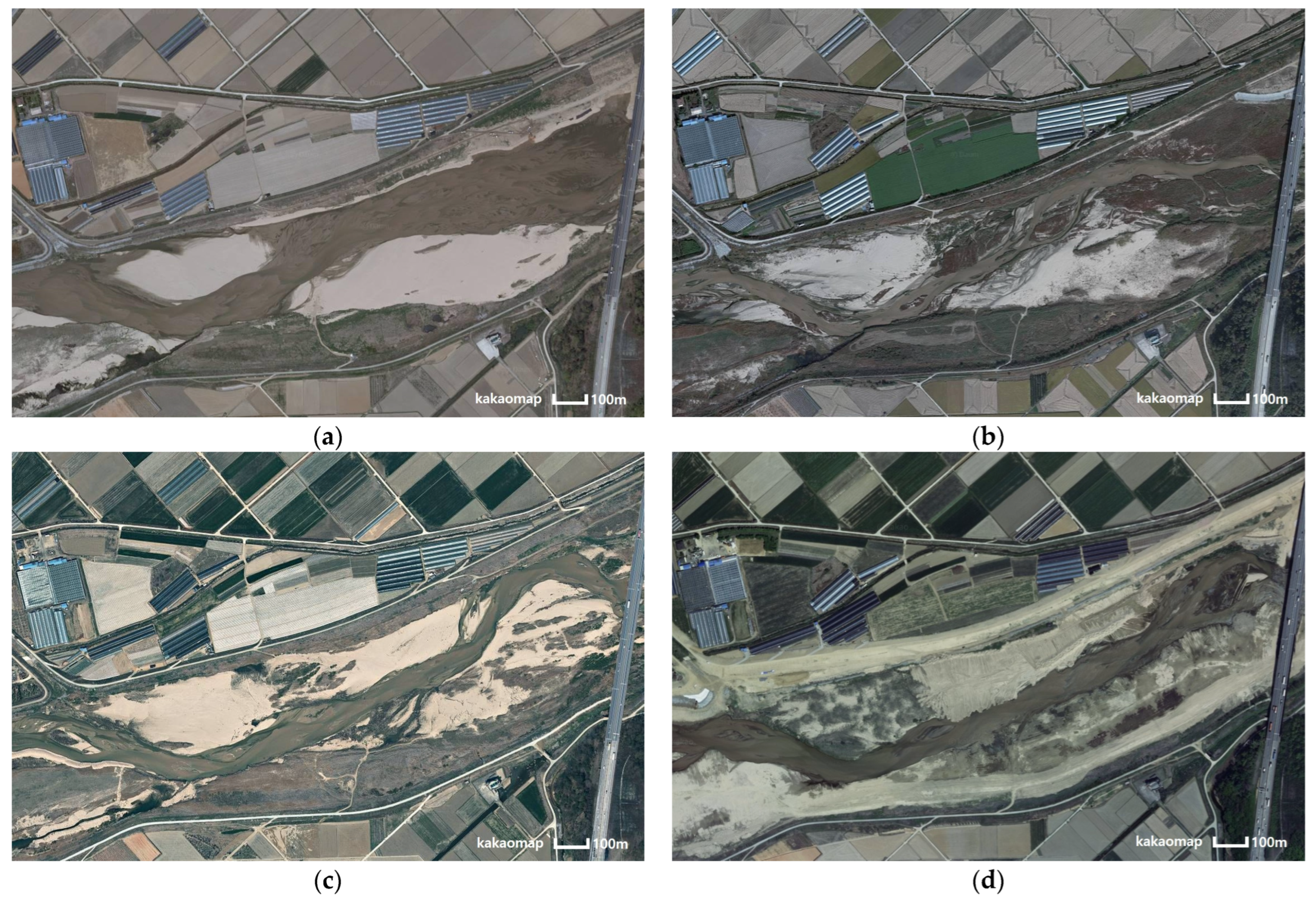
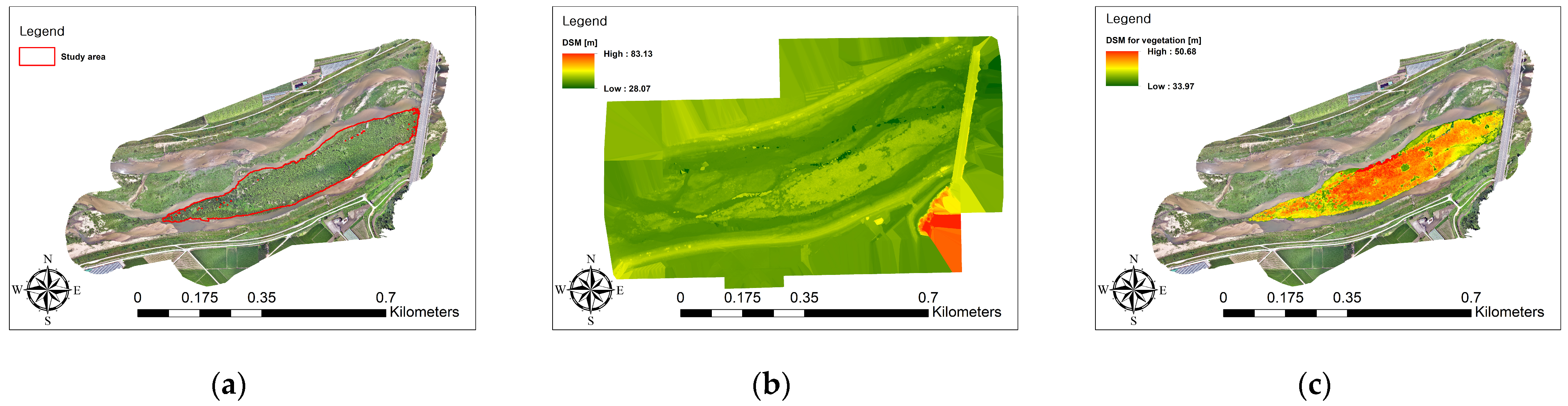
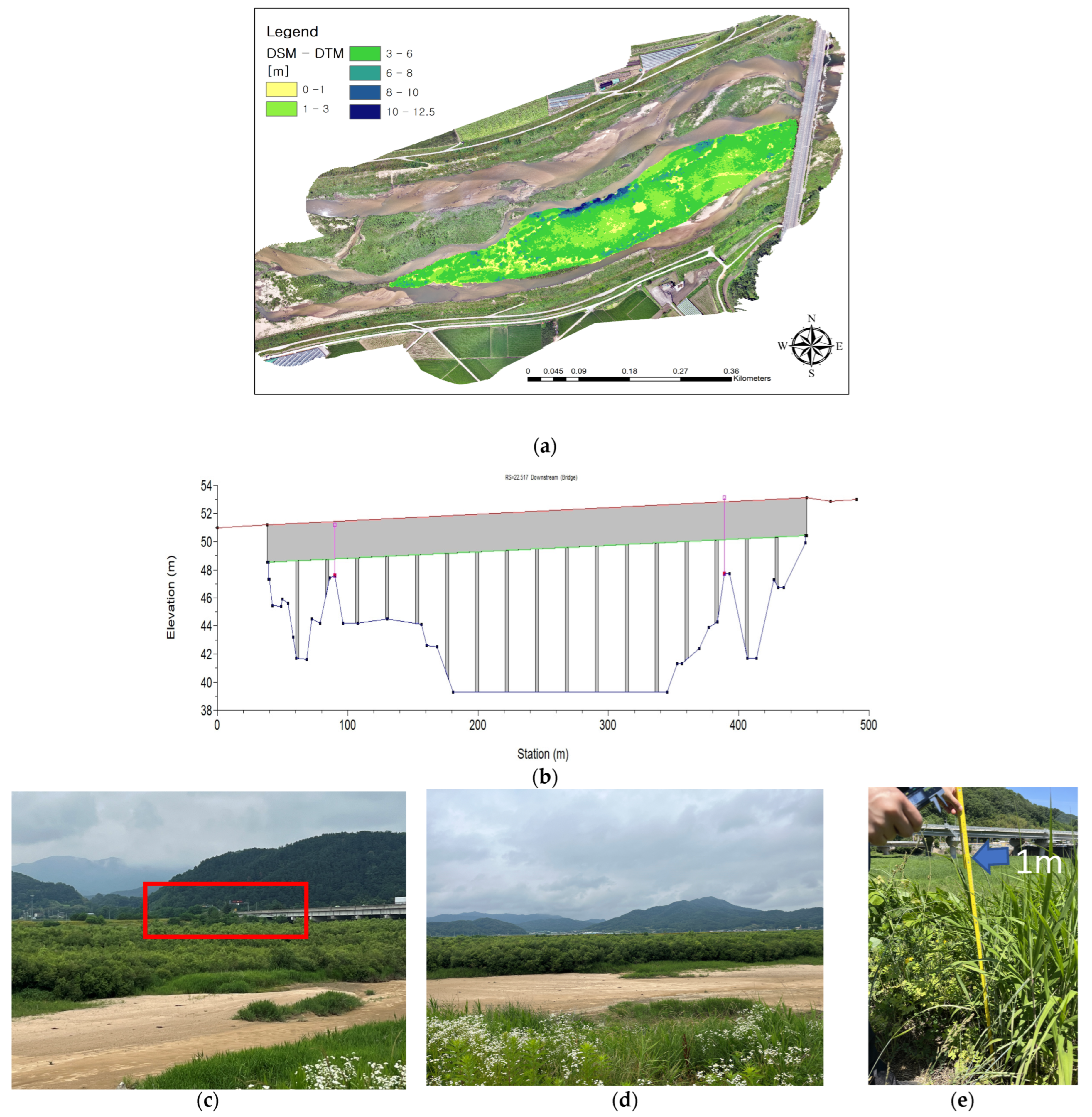
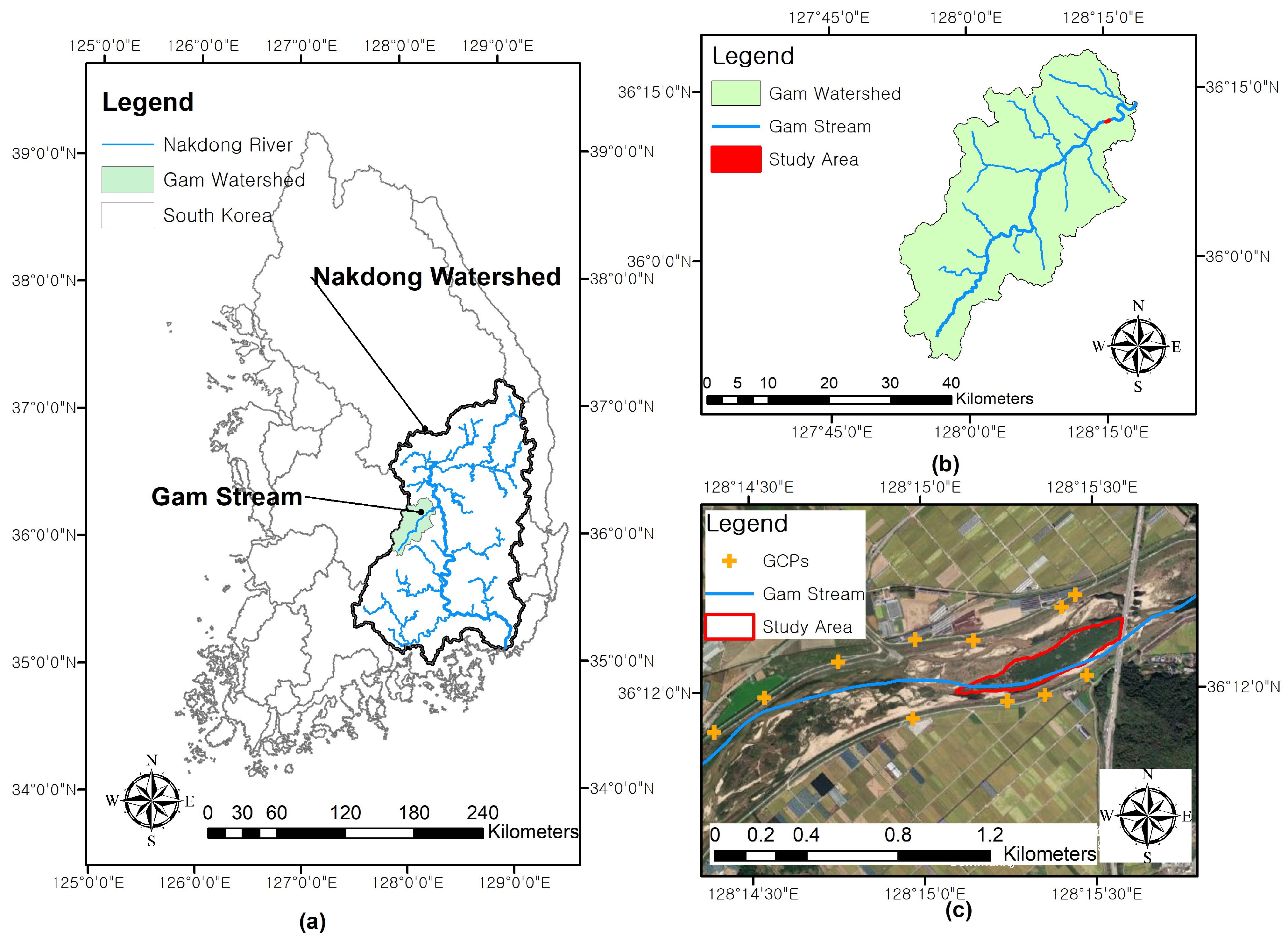
2.1. Target Section and Field Survey

The Gam stream basin is the first tributary of the Nakdong River in South Korea, located in the southeast of the country (Figure 1). The river length of Gam stream is approximately 28 km, and the basin area is 328.70 km2. The majority of the basin is occupied by agricultural fields and forests, with the urbanized/dry land area accounting for 1.6% [39].
The Gyeongsangbuk-do region, where the Gam stream basin is located, experiences recurring flood damage due to annual typhoons. The area is known for plant species like Salix gracilistyla, Phragmites japonicus, and Typha orientalis, which form dominant populations [39]. In comparison to urban rivers, the majority of the Gam stream basin consists of non-urbanized terrain, such as mountains or farmlands, preserving its natural riverbed. However, recently, due to stability issues caused by plant communities along the riverbanks, plants are being removed physically by uprooting or cutting stems [39]. An analysis of the river development trends of the Gam stream basin from 2008 to 2021 showed that, originally, the basin was primarily composed of sandy riverbanks without vegetation influx. However, an influx of vegetation occurred over time, and by 2021, vegetation banks occupied most of the riverbed, as shown in Figure 2. The impact of the physical removal of vegetation was temporary, and the river eventually restored its original nature due to natural succession. Therefore, selecting and designating specific vegetation sections as focused management areas could effectively suppress unnecessary riparian vegetation and plant damage. This study proposed a method to analyze the volume and shape of vegetation. A section near Seomsan Gam stream bridge in the Gam stream basin was selected as the research target issue (Figure 2). This section has maintained a relatively natural state, but it faces challenges due to vegetation communities. Its topographical characteristics have meant that the basin frequently suffered significant damage caused by large typhoons. Gamcheon City, which includes the confluence of the Jikjisacheon Stream, has suffered particularly heavy damage due to its low-altitude topography. Meanwhile, as shown in Figure 2, it is changing from a “White River” in 2008 (Figure 2a) to a “Green River” in 2021 (Figure 2f), and after 2016, more than 60% of rivers converted to plants on average. There are reasons to be optimistic about the function of stream vegetation; however, these functions inherently involve the increase in flood level that is caused by the decrease in flow rate. This also factored into the selection of the basin as this study’s target area.
On 10 July 2023, a total of 37,042 images with a video resolution of 3840 × 2160 and a focal length 24 mm were acquired using the DJI Mavic 3 with 20 MP, a Hasselblad camera with a 4/3″ CMOS sensor, which could improve clarity and accuracy using Hasselblad’s Natural Colour Solution in in the experimental target area [41]. To generate a 3D point cloud with more accurate location information from images taken at an altitude of approximately 70 m, a total of 11 ground control points (GCPs) were installed across the river area, distributed on embankments, inner banks, and outer banks. The GCPs were directly installed using RTK-GPS, and the results of the installation are presented in Table 1 and Figure 1c.
The Pix4D Mapper Version 4.6.4 was used to generate a point cloud using the images obtained from the drone (Figure 3). The image quality, data, camera optimization, and matching quality used to verify the quality of the generated point cloud produced satisfactory results, and the georeferencing mean RMS error, which is a standard for location accuracy, was 0.0487 m. A 3D point cloud was generated using the SFM method from the overlapped results of the images taken by the drone. The analysis was conducted on an area that, while exhibiting vigorous vegetation growth, also had high image overlap and low light reflection, making it suitable for representing the vegetation patch (red circle in Figure 3a).

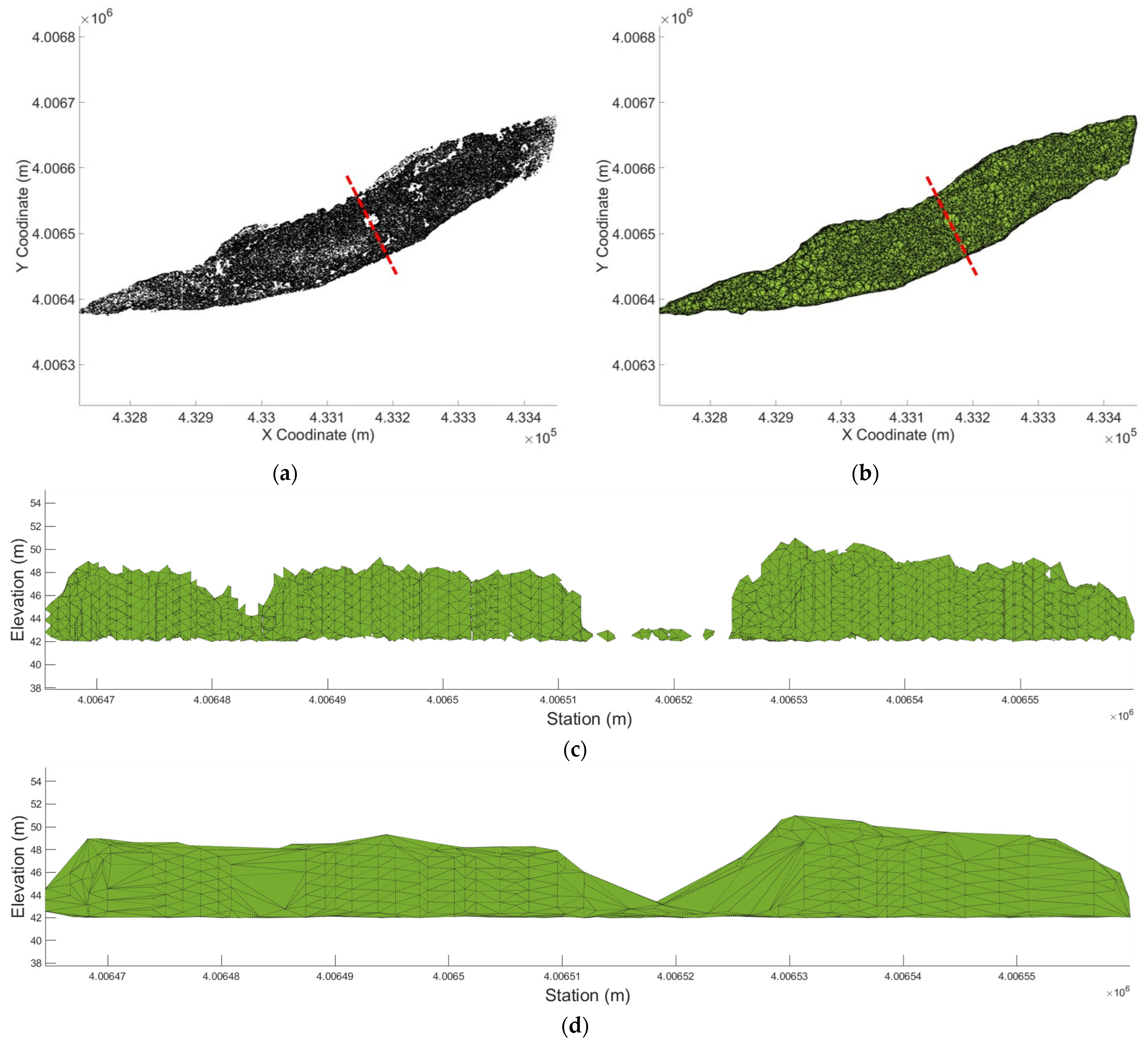
2.2. 3D Point Cloud Editing
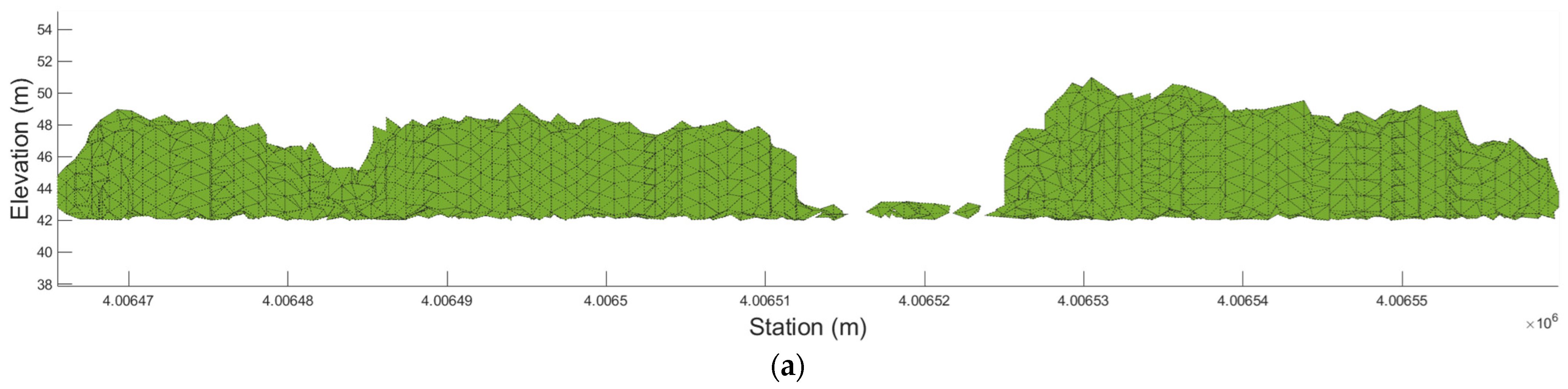
The measured 3D point cloud underwent post-processing using the software CloudCompare (2.12 alpha) after alignment. The initial step in post-processing was to clearly crop the specific target section while simultaneously removing outliers that could cause inaccuracies in volume or morphology. For this purpose, the Statistical Outlier Removal (SOR) method was used to filter out outlier data points. The SOR method calculated the average distance between each point in the initial point cloud and its nearest neighbors, then considered points that deviated from a set standard deviation defined through a Gaussian distribution as outliers and removed them [42]. The SOR filter first calculates the average distance of each point to its neighbors through a k-nearest neighbor search function. If this distance is greater than the average distance derived from all points in the data set plus the standard deviation (σ) of the average distance, the point is considered an outlier [43]. However, the raw initial data of the collected point cloud may not be sufficiently cleaned of outliers with a single application of the SOR process; thus, repeated SOR operations may be necessary in some cases [42]. In Boothroyd [42], up to 20% of the points were removed upon the first application of SOR, and up to 15% on the second application. For the data in this study, about 27 million initial data points were reduced to about 9 million after three filtering processes. However, it is known that if applied more than three times, the edges of the target object begin to be removed, meaning that no real benefit is being offered. At the patch size in particular, the stem shape of the vegetation was not properly represented. The point cloud was organized through a single SOR process to remove outliers from the measured raw data used while using as many points as possible. Additionally, to compensate for the limitation of unnecessarily collecting too many points that did not significantly enhance the results but did waste processing time, a process was employed to remove similar data within a certain space. The data processed in this manner were used for the final volume calculation, comprising 97,361 points (Table 2).
The point cloud measured through the UAV captured the coordinate information of the vegetation patch surface. The vegetation patch would have a hollow shape if it were represented by the directly measured data as the data inside the patch cannot be physically measured from the sky. To overcome this limitation, interpolation was performed from the highest z-coordinate based on each point’s x–y coordinates to the lowest point (reference point). Details regarding the data used in the final analysis are shown in Table 2. The point dimensions in Table 2 refer to the edges of each axis. The sampling and editing process from the raw data did not significantly affect the edges in a way that was important for volume estimation.

2.3. Alpha Shape

Each 3D point cloud collected using a UAV was composed of simply scattered points and did not constitute lines, surfaces, or shapes. Therefore, a reconstruction process was necessary to reconstruct the shape of the desired object. Among them, notable methods included using a convex hull, alpha shape, and voxel [22,23,30,44,45,46,47,48]. While convex hull and alpha shapes connected edge points, the convex hull method connected the exterior points with straight lines, creating limitations in representing rugged objects. In contrast, the alpha shape is a method for reconstructing points composed in 2D or 3D from a discrete space point set. First introduced by Edelsbrunner et al. [44,47], the alpha shape has since been expanded to higher dimensions as a geometric tool for inferring the shape of a point set [41,44]. An alpha shape forms on the boundary of the alpha-complex, which is a sub-complex of the Delaunay triangulation for a given point set [47]. Essentially, the alpha shape composes the boundary region or volume that surrounds a 2D or 3D point set, as shown in Figure 4. For a given set of points in space, a very rough boundary surface to a very refined optimal range around that point could be defined by the parameter alpha (Figure 4). To conduct this, a circle with a radius alpha that connects the contours of two randomly selected points was drawn, forming a 2D or 3D object surrounded by multiple circles. This generated a larger alpha result with a rougher fit, whereas a smaller alpha produces a finer fit (in [46], Figure 4). The level of fine-tuning required for the volume of the 3D alpha shape to match the volume of that alpha shape can be considered a measure of shape complexity. The more complex the object, the more optimal alpha shape adjustment is required.
The result of applying the alpha shape can either represent the optimal shape based on alpha or, if an alpha is set too low, a smaller volume can be created [45]. That is, if the alpha used to construct the alpha shape for an irregular and convex object is too large, it will occupy a volume larger than the actual size. Conversely, an excessively refined alpha shape could have a volume smaller than the original structure. Ultimately, the volume of the alpha shape at the optimal level of refinement and the sample volume could be the same, and finding the optimal alpha was to be prioritized.

3. Results

3.1. Vegetation Volume Estimation Results Based on DSM and DTM

Stereophotogrammetry uses several overlapped images to estimate the three-dimensional coordinates of points, creating point clouds and a digital surface model (DSM) that shows the height values of trees or buildings. After the drone photography, a DSM with a resolution of 3.3 cm was created based on the produced point cloud (Figure 5b), and the surface elevation values of the research area, mostly composed of vegetation, appeared to be between 40.0 m and 52.5 m.
The created point cloud was sorted into the following categories based on machine learning techniques incorporating geometry and color information: soil, road, vegetation, building, and artificially constructed objects [46]. After classifying the created point cloud into the noted categories, a DTM was constructed based on the classification results. In the area of study for this research, a DTM with a resolution of 1 cm was produced based on the points classified as vegetation and soil. Boundaries for the section to calculate the vegetation volume were initially extracted from the post-processed point cloud at different resolutions to directly compare with the vegetation volume estimated using the alpha shape. Ultimately, to compare with the vegetation volume calculated using the point cloud, the height of the vegetation was determined by subtracting the DTM from the DSM in the area of interest (Figure 6).
To validate the height of vegetation, the field survey and the reference of Basic Plan for the Gam Stream Development and Management and actual field survey results were used. Based on the Basic Plan for the Gam Stream Development and Management report, the height from riverbed to bridge was about 42 m to 49 m (right side in Figure 6b). Most trees (Figure 6d), which are inconvenient to access and difficult to measure in the field without specific measuring equipment, have a height of approximately 3 to 6 m (Figure 6a); based on the report, these results seem reasonable. Additionally, for some trees with a height of 8–10 m, the red square area in Figure 6c was well delineated, and the remaining grasslands with a height of approximately 1 m were also well represented, which was the result of actual measurements at accessible locations (Figure 6d). From these results, it appears that the survey results reflect the information on actual vegetation well, and the volume of the vegetation was calculated by multiplying the average difference by the area (Table 3).
When the boundary of the research area was extracted at high resolution, areas without point cloud generation were excluded from the analysis, resulting in a reduced area (Figure 7a–c). However, the areas without point clouds and which were not included in the area calculation were mostly areas without vegetation, so the average height of the vegetation (DTM-DSM) increased (Figure 7d). For this reason, the vegetation volume calculated using the area and average height of the vegetation did not show significant differences due to changes in resolution (Table 3).

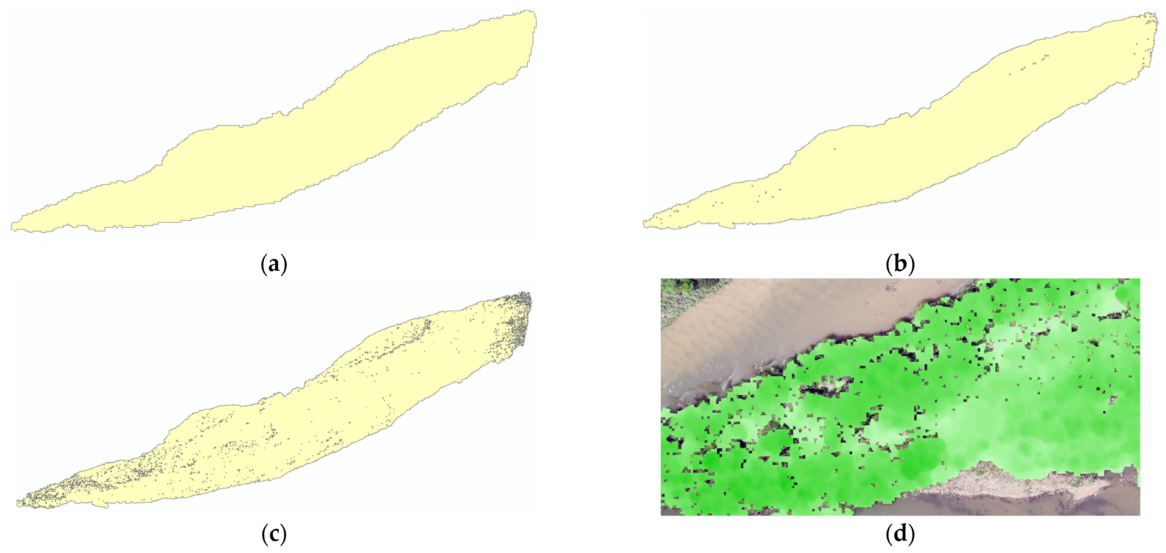
3.2. Results of Volume Estimation by the Alpha Shape Method

The volume estimation by the alpha shape method for different radii (α) is shown in Figure 8 and Figure 9. Figure 8 represents the top view and cross-sectional results of volume estimation by radius 0.7 and 10. The volume was estimated considering that the target object was unstructured. It was determined whether the appropriate radius was 1 or 10, regardless of the object’s size. Objects with more complex edges require smaller radii, while less complex edges require larger radii. If the vegetation patch has been a large cuboid, it is not necessary to be overly concerned with the alpha radius. Nevertheless, as we know, finding the appropriate alpha radius when edges are jumbled makes sense. This study finds appropriate values for an unlimited alpha radius range and estimates the most optimized volume. Due to the range covered, which changed significantly depending on the radius α used in the alpha shape method (especially for larger subjects like the one in this study), the volume at α = 0.7 and α = 10 was 113,035 and 377,582 m3, respectively, a difference of approximately 260,000 m3.
Figure 8a shows how an inaccurate representation of the true shape results from using a radius that is too small to fill the actual object. That is, if a very small α like 0.6 is set, it will not encompass the entire target object, preventing an accurate representation of the actual volume. Conversely, as shown in Figure 8d, a too-large radius results in volume estimation even for areas that are actually empty. Using an α value that is too large would overestimate and inaccurately represent the object’s shape. These results highlight the importance of setting the alpha radius. Comparing the results of the volume estimation by alpha radius (Figure 9), when the radius was set to 0.8, the volume of the vegetation patch was 246,413 m3, which is the most similar value to the patch volume based on DSM and DTM.
The vegetation patch volume estimation based on DSM and DTM was a result that did not consider the voids inside the vegetation. Therefore, it can be presumed to be overestimated compared to the actual volume. Hence, the volume estimation result using Radius 0.8 in the alpha shape method was also expected to be overestimated. Considering this estimation and the radius range that was too small to be properly implemented, the optimal alpha radius for this research subject could be recommended as 0.75, and the 3D image of the implemented vegetation patch using this is as shown in Figure 10. By comparing the implemented vegetation patch and the orthoimage generated from the drone capture results of the area, it was confirmed that areas without actual vegetation were reproduced, and the amount of vegetation excluding these areas was estimated.

4. Discussion

Since the volume estimation method by alpha shape was based on point cloud data, using appropriate points was critical. Although point clouds had the advantage of easily generating large amounts of data, they could contain outliers and unnecessary data, so a separate editing process was required. In this process, there was no need to use millions of data points to extract regular and correct objects. However, care was to be taken not to delete points necessary for shape implementation during the outlier removal process. Many studies have researched methods on how to remove outliers to extract the minimum necessary data. This process significantly influences the success or failure of the research.
In this study, the SOR technique to remove outliers was used. Data collection took place outdoors, and since the desired object was not of a fixed shape, data editing was completed cautiously. Additionally, efforts were made to ensure that necessary data were not deleted during the extensive editing process. In this study, the volume of the vegetation patch was estimated using point clouds refined through a minimal SOR process. Comparing it with the initial data in Table 2 confirmed that the size did not change significantly even after successive SOR processes. Since the edges did not change significantly, it was judged that there would be no significant difference when estimating the volume. However, when actually calculating the volume, it was observed that the estimated volume decreased as the SOR process progressed (Figure 11). For the proposed optimal alpha radius of 0.75 for the research subject, there was a difference of 17,347 m3 in volume after the 1st and 2nd SOR, and a difference of 36,312 m3 after the 3rd SOR.
However, caution is clearly needed when considering the volume estimation results by cross-sectional area for each SOR process (Figure 12) as the required area during the SOR process may not be included. In fact, the vegetation patch on the left side of the image was not interrupted, but as the SOR process progressed, necessary points were removed, resulting in a disconnected shape. Thus, there was no universal definition of how many times the SOR process should be undertaken to be optimal, and depending on the target object and measurement environment, the optimal results could vary significantly, so caution was essential. Using the volume estimation results to discern the optimum would result in the usage of an inappropriate alpha radius, which could produce inaccurate results.

5. Conclusions

Based on established data, UAV photogrammetry was used to develop and align 3D point clouds and estimate the amount of riparian vegetation at the patch scale. Initially, a UAV was used to capture 37,042 images of the target cross-section, which were then used to generate a point cloud with precise location information. To ensure more precise location information of the 3D point cloud, 11 GCPs were operated. The point cloud was generated and aligned using Pix4D Mapper, confirming that there were no issues with image quality, data, camera optimization, matching quality, or location accuracy. Among the results generated through the post-processing process, an area that accurately represents the vegetation patch of the analysis target area was selected, and the amount of riparian vegetation was finally estimated using 97,361 points.
The first method to estimate the volume of riparian vegetation used the DSM and DTM developed from the 3D point cloud. Specifically, the DSM was directly developed from the point cloud, and subsequently, the point cloud was classified into soil, road, vegetation, building, and artificially created objects to develop the DTM. To compare with the volume estimation results by alpha shape, the difference between DSM and DTM was assumed to be vegetation, and the validation of height of vegetation (DSM-DTM) with the reference and field survey was reasonable. Using this result, the vegetation volume (approximately 242,000 m3) was calculated by multiplying the average difference value by the area of the target section. The volume estimation results by alpha radius were compared with methods using volume estimation by alpha shape. The analysis results showed that a small radius cannot properly represent the intended object or produces unrealistically low volumes (about 7610 m3 at radius = 0.6, error 97%). In contrast, a large radius overestimates the object’s shape (about 377,582 m3 at radius = 10, error 56%), but it has been observed that the estimated volume does not increase infinitely as the radius increases. When compared to the orthoimages generated from actual drone images, the most meaningful radius was found to be 0.75. It was confirmed that a thorough review of the radius value is necessary when estimating the amount of vegetation using the alpha form. Additionally, while outlier removal and handling of large amounts of meaningless data were essential, changes in volume owing to the actual alpha radius values had less of an impact when using point clouds to estimate the volume of an object. However, even as the radius value increases and the volume does not continuously increase, it was observed that the volume decreases as noise processing increases. This result indicates the importance of ensuring that essential points are not removed during data processing.
The research results of this study are expected to serve as basic data for managing riparian vegetation that excessively adheres to rivers. If the exact value of the target vegetation patch is known, deriving an accurate value for the radius will be essential. However, we recognized the limitations of not knowing the actual value of natural vegetation patches and began research to find realistic alternatives. In reality, calculating the amount of vegetation planted in a space of approximately 70,000 m2 is only possible by cutting down all the vegetation and measuring it on a laboratory scale. We recognized and accepted these limitations in the field and tried to present approximate values that could be realistically used. Therefore, if someone needs to estimate the approximate volume of large vegetation patches like this (for dense and lush vegetation patches, like Figure 6c–e), it is recommended to use 0.75.
The volume estimation method using point clouds obtained from UAV photogrammetry and alpha shape examined in this study is expected to be useful, especially when access is impossible due to spatial constraints or when there are temporal and economic limitations due to a large scale. Although the technology for estimating volume based on drone measurements and that for estimating volume based on the alpha shape have both been introduced previously, they target standardized objects in some cases. Additionally, the method of estimation through drone surveying is required for non-standard objects, such as river vegetation. Calculating river vegetation amount, which requires the exact area and height of the object, is bound to vary depending on the field survey basis. Therefore, the method of using point clouds and alpha shapes based on drone surveying in calculating river vegetation amount, as achieved in this study, is an improved result for irregular objects. In addition, the two techniques used in the existing study can be fully applied. Also, improvements and alternatives are suggested, noting that caution is needed in alpha value selection and preprocessing. Advancements in technology to accurately estimate the volume of vegetation will be used to determine how much vegetation needs to be removed for flood safety and can be used to manage spaces blocked by vegetation for flood level management and to determine the adhesion scale of different types of vegetation.

Author Contributions

Conceptualization, E.J.; Formal analysis, writing—review and editing, Investigation, Data Curation, W.K. and E.J. All authors have read and agreed to the published version of the manuscript.

Funding

This research was carried out under the KICT Research Program (project no. 20230115-001, Development of IWRM-Korea Technical Convergence Platform Based on Digital New Deal), funded by the Ministry of Science and ICT. This research was supported by the National Research Foundation of Korea (NRF) grant funded by the Korea government (MSIP) (NRF-2019R1C1C1009719).

Institutional Review Board Statement

Not applicable.

Informed Consent Statement

Not applicable.

Data Availability Statement

The data presented in this study are available on request from the corresponding author. The data are not publicly available due to security reasons from research funding agencies.

Conflicts of Interest

The authors declare no conflict of interest.

References

  1. Rominger, J.T.; Lightbody, A.F.; Nepf, H.M. Effects of added vegetation on sand bar stability and stream hydrodynamics. J. Hydraul. Eng. 2010, 136, 994–1002. [Google Scholar] [CrossRef]
  2. Surian, N.; Barban, M.; Ziliani, L.; Monegato, G.; Bertoldi, W.; Comiti, F. Vegetation turnover in a braided river: Frequency and effectiveness of floods of different magnitude. Earth Surf. Process. Landf. 2015, 40, 542–558. [Google Scholar] [CrossRef]
  3. Jin, S.N.; Cho, K.H. Expansion of riparian vegetation due to change of flood regime in the Cheongmi-cheon stream, Korea. Ecol. Resil. Infrastruct. 2016, 3, 322–326. [Google Scholar] [CrossRef]
  4. Kim, W.; Kim, S. Analysis of the riparian vegetation expansion in middle size rivers in Korea. J. Korea Water Resour. Assoc. 2019, 52, 875–885. [Google Scholar]
  5. Kim, W.; Kim, S. Riparian vegetation expansion due to the change of rainfall pattern and water level in the river. Ecol. Resil. Infrastruct. 2020, 7, 238–247. [Google Scholar]
  6. Ji, U.; Järvelä, J.; Västilä, K.; Bae, I. Experimentation and modeling of reach-scale vegetative flow resistance due to willow patches. J. Hydraul. Eng. 2023, 149, 04023018. [Google Scholar] [CrossRef]
  7. Lee, C.; Kim, D.G.; Hwang, S.Y.; Kim, Y.; Jeong, S.; Kim, S.; Cho, H. Dataset of long-term investigation on change in hydrology, channel morphology, landscape and vegetation along the Naeseong stream (II). Ecol. Resil. Infrastruct. 2019, 6, 34–48. [Google Scholar]
  8. Woo, H.; Cho, K.H.; Jang, C.L.; Lee, C.J. Fluvial processes and vegetation-research trends and implications. Ecol. Resil. Infrastruct. 2019, 6, 89–100. [Google Scholar]
  9. Woo, H.; Park, M. Cause-based categorization of the riparian vegetative recruitment and corresponding research direction. Ecol. Resil. Infrastruct. 2016, 3, 207–211. [Google Scholar] [CrossRef]
  10. Woo, H.; Park, M.; Cheong, S.J. A preliminary investigation on patterns of riparian vegetation establishment and typical cases in Korea. In Proceedings of the Annual Conference of Korea Water Resources Association, Pyungchang, Republic of Korea, 8–12 November 2009; Korea Water Resources Association: Seoul, Republic of Korea, 2009; pp. 474–478. [Google Scholar]
  11. Wang, Y.; Fu, B.; Liu, Y.; Li, Y.; Feng, X.; Wang, S. Response of vegetation to drought in the Tibetan plateau: Elevation differentiation and the dominant factors. Agric. For. Meteorol. 2021, 306, 108468. [Google Scholar] [CrossRef]
  12. Lama, G.F.C.; Errico, A.; Francalanci, S.; Chirico, G.B.; Solari, L.; Preti, F. Hydraulic modeling of field experiments in a drainage channel under different riparian vegetation scenarios. In Innovative Biosystems Engineering for Sustainable Agriculture, Forestry and Food Production: International Mid-Term Conference 2019 of the Italian Association of Agricultural Engineering (AIIA); Springer International Publishing: Berlin/Heidelberg, Germany, 2020; pp. 69–77. [Google Scholar] [CrossRef]
  13. Symmank, L.; Natho, S.; Scholz, M.; Schröder, U.; Raupach, K.; Schulz-Zunkel, C. The impact of bioengineering techniques for riverbank protection on ecosystem services of riparian zones. Ecol. Eng. 2020, 158, 106040. [Google Scholar] [CrossRef]
  14. Naiman, R.J.; Decamps, H.; Pollock, M. The role of riparian corridors in maintaining regional biodiversity. Ecol. Appl. 1993, 3, 209–212. [Google Scholar] [CrossRef] [PubMed]
  15. Nilsson, C.; Svedmark, M. Basic principles and ecological consequences of changing water regimes: Riparian plant communities. Environ. Manag. 2002, 30, 468–480. [Google Scholar] [CrossRef] [PubMed]
  16. Tockner, K.; Stanford, J.A. Riverine flood plains: Present state and future trends. Environ. Conserv. 2002, 29, 308–330. [Google Scholar] [CrossRef]
  17. Catterall, C.P.; Lynch, R.; Jansen, A. Riparian wildlife and habitats. In Principles for Riparian Lands Management; Lovett, S., Price, P., Eds.; Land and Water Australia: Canberra, Australia, 2007; pp. 141–158. [Google Scholar]
  18. Blentlinger, L.; Herrero, H.V. A tale of grass and trees: Characterizing vegetation change in Payne’s Creek National Park, Belize from 1975 to 2019. Appl. Sci. 2020, 10, 4356. [Google Scholar] [CrossRef]
  19. Catford, J.A.; Jansson, R. Drowned, buried and carried away: Effects of plant traits on the distribution of native and alien species in riparian ecosystems. New Phytol. 2014, 204, 19–36. [Google Scholar] [CrossRef] [PubMed]
  20. Garssen, A.G.; Verhoeven, J.T.; Soons, M.B. Effects of climate-induced increases in summer drought on riparian plant species: A meta-analysis. Freshw. Biol. 2014, 59, 1052–1063. [Google Scholar] [CrossRef]
  21. Rohde, S.; Schütz, M.; Kienast, F.; Englmaier, P. River widening: An approach to restoring riparian habitats and plant species. River Res. Appl. 2005, 21, 1075–1094. [Google Scholar] [CrossRef]
  22. Jang, E.K.; Ahn, M. Estimation of single vegetation volume using 3D point cloud-based alpha shape and voxel. Ecol. Resil. Infrastruct. 2021, 8, 204–211. [Google Scholar]
  23. Ahn, M.; Jang, E.K.; Bae, I.; Ji, U. Reconfiguration of physical structure of vegetation by voxelization based on 3D point clouds. KSCE J. Civ. Environ. Eng. Res. 2020, 40, 571–581. [Google Scholar]
  24. Jang, E.K.; Ahn, M.; Ji, U. Introduction and application of 3D terrestrial laser scanning for estimating physical structurers of vegetation in the channel. Ecol. Resil. Infrastruct. 2020, 7, 90–96. [Google Scholar]
  25. Yan, G.; Li, L.; Coy, A.; Mu, X.; Chen, S.; Xie, D.; Zhang, W.; Shen, Q.; Zhou, H. Improving the estimation of fractional vegetation cover from UAV RGB imagery by colour unmixing. ISPRS J. Photogramm. 2019, 158, 23–34. [Google Scholar] [CrossRef]
  26. Yan, G.; Hu, R.; Luo, J.; Weiss, M.; Jiang, H.; Mu, X.; Xie, D.; Zhang, W. Review of indirect optical measurements of leaf area index: Recent advances, challenges, and perspectives. Agric. For. Meteorol. 2019, 265, 390–411. [Google Scholar] [CrossRef]
  27. Qiao, L.; Zhao, R.; Tang, W.; An, L.; Sun, H.; Li, M.; Wang, N.; Liu, Y.; Liu, G. Estimating maize LAI by exploring deep features of vegetation index map from UAV multispectral images. Field Crops Res. 2022, 289, 108739. [Google Scholar] [CrossRef]
  28. Vicari, M.B.; Disney, M.; Wilkes, P.; Burt, A.; Calders, K.; Woodgate, W. Leaf and wood classification framework for terrestrial LiDAR point clouds. Methods Ecol. Evol. 2019, 10, 680–694. [Google Scholar] [CrossRef]
  29. Nguyen, V.T.; Fournier, R.A.; Côté, J.F.; Pimont, F. Estimation of vertical plant area density from single return terrestrial laser scanning point clouds acquired in forest environments. Remote Sens. Environ. 2022, 279, 113115. [Google Scholar] [CrossRef]
  30. Soma, M.; Pimont, F.; Dupuy, J.L. Sensitivity of voxel-based estimations of leaf area density with terrestrial LiDAR to vegetation structure and sampling limitations: A simulation experiment. Remote Sens. Environ. 2021, 257, 112354. [Google Scholar] [CrossRef]
  31. Béland, M.; Kobayashi, H. Mapping forest leaf area density from multiview terrestrial LiDAR. Methods Ecol. Evol. 2021, 12, 619–633. [Google Scholar] [CrossRef]
  32. Halubok, M.; Kochanski, A.K.; Stoll, R.; Bailey, B.N. Errors in the estimation of leaf area density from aerial LiDAR data: Influence of statistical sampling and heterogeneity. IEEE Trans. Geosci. Remote Sens. 2021, 60, 1–14. [Google Scholar] [CrossRef]
  33. Wei, S.; Yin, T.; Dissegna, M.A.; Whittle, A.J.; Ow, G.L.F.; Yusof, M.L.M.; Lauret, N.; Gastellu-Etchegorry, J.P. An assessment study of three indirect methods for estimating leaf area density and leaf area index of individual trees. Agric. For. Meteorol. 2020, 292–293, 108101. [Google Scholar] [CrossRef]
  34. Polat, N.; Uysal, M. An experimental analysis of digital elevation models generated with LiDAR data and UAV photogrammetry. J. Indian Soc. Remote Sens. 2018, 46, 1135–1142. [Google Scholar] [CrossRef]
  35. Nikolakopoulos, K.G.; Kyriou, A.; Koukouvelas, I.K. Developing a guideline of unmanned aerial vehicle’s acquisition geometry for landslide mapping and monitoring. Appl. Sci. 2022, 12, 4598. [Google Scholar] [CrossRef]
  36. Mohan, M.; Leite, R.V.; Broadbent, E.N.; Wan Mohd Jaafar, W.S.; Srinivasan, S.; Bajaj, S.; Dalla Corte, A.P.; do Amaral, C.H.; Gopan, G.; Saad, S.N.M.; et al. Individual tree detection using UAV-Lidar and UAV-SfM data: A tutorial for beginners. Open Geosci. 2021, 13, 1028–1039. [Google Scholar] [CrossRef]
  37. Chen, S.; McDermid, G.J.; Castilla, G.; Linke, J. Measuring vegetation height in linear disturbances in the boreal forest with UAV photogrammetry. Remote Sens. 2017, 9, 1257. [Google Scholar] [CrossRef]
  38. Giannetti, F.; Chirici, G.; Gobakken, T.; Næsset, E.; Travaglini, D.; Puliti, S. A new approach with DTM-independent metrics for forest growing stock prediction using UAV photogrammetric data. Remote Sens. Environ. 2018, 213, 195–205. [Google Scholar] [CrossRef]
  39. Ministry of Land (MoL). Infrastructure and Transport Gamcheon River Maintenance Basic Plan, Ministry of Land; Ministry of Land (MoL): Sejong, Republic of Korea, 2020.
  40. Kakao Map. Available online: https://map.kakao.com/ (accessed on 15 December 2023).
  41. Nwaogu, J.M.; Yang, Y.; Chan, A.P.; Chi, H.L. Application of drones in the architecture, engineering, and construction (AEC) industry. Autom. Constr. 2023, 150, 104827. [Google Scholar] [CrossRef]
  42. Boothroyd, R. Flow-Vegetation Interactions at the Plant-Scale: The Importance of Volumetric Canopy Morphology on Flow Field Dynamics. Ph.D. Thesis, Durham University, Durham, UK, 2017. [Google Scholar]
  43. ColudCompare (Webpage) SOR Filter. Available online: https://www.cloudcompare.org/doc/wiki/index.php?title=SOR_filter#Description (accessed on 15 December 2023).
  44. Edelsbrunner, H.; Kirkpatrick, D.; Seidel, R. On the shape of a set of points in the plane. IEEE Trans. Inf. Theor. 1983, 29, 551–559. [Google Scholar] [CrossRef]
  45. Becker, C.; Häni, N.; Rosinskaya, E.; d’Angelo, E.; Strecha, C. Classification of aerial photogrammetric 3D point clouds. arXiv 2017, arXiv:1705.08374. [Google Scholar] [CrossRef]
  46. Gardiner, J.D.; Behnsen, J.; Brassey, C.A. Alpha shapes: Determining 3D shape complexity across morphologically diverse structures. BMC Evol. Biol. 2018, 18, 184. [Google Scholar] [CrossRef]
  47. Xu, X.; Harada, K. Automatic surface reconstruction with alpha-shape method. Vis. Comput. 2003, 19, 431–443. [Google Scholar] [CrossRef]
  48. Edelsbrunner, H.; Mücke, E.P. Three-dimensional alpha shapes. ACM Trans. Graph. 1994, 13, 43–72. [Google Scholar] [CrossRef]
Figure 1. The study area of this study: (a) location of Gam watershed, (b) location of study area, and (c) location of Ground Control Points.
Applsci 14 00020 g001
Figure 2. Yearly images of the research target section: (a) 2008, (b) 2009, (c) 2014, (d) 2017, (e) 2019, and (f) 2021. Aerial imagery from KAKAO map [40].
Applsci 14 00020 g002aApplsci 14 00020 g002b
Figure 3. Point cloud extracted from the drone: (a) raw data and the target range with red dash line (b) cropped image of the target section.
Applsci 14 00020 g003
Figure 4. Example of volume estimation by original shape and alpha shape method according to radius (α).
Applsci 14 00020 g004
Figure 5. (a) Orthographic image of the research area in Gam stream, (b) digital surface model created from the point cloud, and (c) digital surface model for vegetation.
Applsci 14 00020 g005
Figure 6. (a) Result of subtracting DTM from the DSM of the research area, (b) distance information from riverbed to bridge, (c,d) photos of study area, and (e) grass height field survey height.
Applsci 14 00020 g006
Figure 7. Boundaries of the research area extracted by resolution (a) 2.4 m, (b) 1.2 m, (c) 0.56 m, and (d) areas excluded from the research area due to a lack of point cloud.
Applsci 14 00020 g007
Figure 8. Volume estimation images by alpha radius (a) top view with radius 0.7, (b) top view with radius 10, (c) cross-sectional image with radius 0.7 at the red dashed line in (a), and (d) cross-sectional image with radius 10 at the red dashed line in (b).
Applsci 14 00020 g008
Figure 9. Results of volume estimation by alpha radius (α).
Applsci 14 00020 g009
Figure 10. (a) 3D vegetation patch implementation result using alpha radius (α = 0.75) and (b) orthoimage of the respective section.
Applsci 14 00020 g010
Figure 11. Volume estimation results by alpha radius (α) for each SOR degree.
Applsci 14 00020 g011
Figure 12. Volume implementation result images when the alpha radius is 0.75: (a) 1st SOR, (b) 2nd SOR, and (c) 3rd SOR.
Applsci 14 00020 g012aApplsci 14 00020 g012b
Table 1. Ground control points for 3D point cloud modeling (Korea 2000/Central Belt 2010 (EGM 96 Geoid).
NameCoordinatesNameCoordinates
X (m)Y (m)Z (m)X (m)Y (m)Z (m)
GCP1313,137.79401,026.0848.44GCP7312,052.35401,082.4049.20
GCP2312,954.72400,941.3448.7GCP8312,388.18401,180.3246.36
GCP3312,791.71400,912.2744.94GCP9312,642.63401,176.6444.58
GCP4312,378.46400,837.2349.33GCP10313,027.94401,321.8144.70
GCP5311,511.35400,776.9949.86GCP11313,087.25401,376.7348.47
GCP6311,731.34400,927.8149.43
Table 2. Initial point information of the 3D point cloud and point information after editing.
Raw Data
(Surface Only)
Sampling by Space
(Surface Only)
Filled Point Data
Raw data27,004,538--
SOR 1st23,882,81697,361446,050
SOR 2nd20,599,44690,762414,791
SOR 3rd18,255,11285,151386,791
Table 3. Area of the research site and the volume of vegetation calculated in the section, extracted by resolution.
Cell SizeMean Elevation of DSM-DTM (m)Standard Deviation of DSM-DTM (m)Area of Study Site
(m2)
Volume
(m3)
0.563.5671.7866,380.4236,779
1.23.5451.7768,545.9242,995
2.43.5421.7570,011.8247,981
Disclaimer/Publisher’s Note: The statements, opinions and data contained in all publications are solely those of the individual author(s) and contributor(s) and not of MDPI and/or the editor(s). MDPI and/or the editor(s) disclaim responsibility for any injury to people or property resulting from any ideas, methods, instructions or products referred to in the content.

