Abstract
Extracting river channels from remote sensing images is crucial for locating river water bodies and efficiently managing water resources, especially in cold and arid regions. The dynamic nature of river channels in these regions during the flood season necessitates a method that can finely delineate the edges of perennially changing river channels and accurately capture information about variable fine river branches. To address this need, we propose a river channel extraction method designed specifically for detecting fine river branches in remote sensing images within cold and arid regions. The method introduces a novel river attention U-shaped network structure (RAU-Net++), leveraging the rich convolutional features of VGG16 for effective feature extraction. For optimal feature extraction along channel edges and fine river branches, we incorporate a CBAM attention module into the upper sampling area at the end of the encoder. Additionally, a residual attention feature fusion module (RAFF) is embedded at each short jump connection in the dense jump connection. Dense skip connections play a crucial role in extracting detailed texture features from river channel features with varying receptive fields obtained during the downsampling process. The integration of the RAFF module mitigates the loss of river information, optimizing the extraction of lost river detail feature information in the original dense jump connection. This tightens the combination between the detailed texture features of the river and the high-level semantic features. To enhance network performance and reduce pixel-level segmentation errors in medium-resolution remote sensing imagery, we employ a weighted loss function comprising cross-entropy (CE) loss, dice loss, focal loss, and Jaccard loss. The RAU-Net++ demonstrates impressive performance metrics, with precision, IOU, recall, and F1 scores reaching 99.78%, 99.39%, 99.71%, and 99.75%, respectively. Meanwhile, both ED and ED′ of the RAU-Net++ are optimal, with values of 1.411 and 0.003, respectively. Moreover, its effectiveness has been validated on NWPU-RESISC45 datasets. Experimental results conclusively demonstrate the superiority of the proposed network over existing mainstream methods.
1. Introduction
As valuable natural resources, rivers occupy a more important position in cold and arid areas [1]. The ecological environment of river basins in cold and arid zones is fragile. The background information of river basins is very complex; however, remote sensing images can comprehensively obtain complex ground information, with the advantages of easy access, short cycles, and rich information [2,3]. Therefore, it is possible to extract real-time, comprehensive, and accurate information about the river channel in cold and arid areas through remote sensing image monitoring, which is of great practical significance for the investigation, monitoring, and protection of water resources in cold and arid areas [4,5].
The current traditional methods for river extraction from remote sensing images include morphology, thresholding, clustering, and classifiers [6]. Kurshid et al. [7] proposed an iterative multiresolution decomposition using texture features combined with morphology to extract rivers from panchromatic satellite images. Zhu He et al. [8] proposed a novel multi-stage river extraction method by combining grayscale thresholding and morphological features and correcting the results using morphological filtering. Yousufi et al. [9] introduced a novel river extraction method that utilizes mathematical morphology training samples, Bayesian classifiers, and dynamically varying filters. This approach involves evaluating morphological erosion and dilation to generate a profile segmentation of the river. Additionally, the Bayesian algorithm is applied to enhance the segmentation results. Rani et al. [10] used segmentation methods such as K-mean clustering and region growth to segment the color components of different regions in the satellite river image for river extraction. All the aforementioned traditional river segmentation methods necessitate the manual selection of feature parameters, limiting their applicability to simple scenes and presenting notable constraints for complex environmental segmentation [11].
In recent years, the application of convolutional neural networks in deep learning has become more and more widespread and has performed well in the task of river segmentation in remote sensing images, achieving better results [12,13]. Yu Long et al. [14] applied a convolutional neural network in the surface river extraction task and the results were significantly better than traditional water extraction methods. However, CNN, as an end-to-end, pixel-to-pixel network, reduces spatial information and increases the number of parameters when using a fully connected layer. In order to solve this problem, Evan Sherhammer et al. [15] proposed a fully convolutional network (FCN) by replacing the fully connected layer with a convolutional layer. With the full convolutional networks proposed, many classical semantic segmentation algorithms, such as Unet, Linknet, PSPnet, Upernet, Deeplabv3+, Manet, Transunet, etc., have been proposed [16]. Among them, Ronneberger et al. [17] proposed a U-shaped structural model UNet based on a fully convolutional network in 2015. UNet is divided into two parts—the encoder and the decoder. The encoder makes constant convolution of the feature map for feature extraction, which preserves the texture detail information, and the decoder performs upsampling to preserve more semantic information. The encoder makes the layer-hopping connection with the decoder to enable the network to have more detailed semantic information. In 2017, Linknet [18] and PSPnet [19] were proposed, respectively. Linknet was proposed by Abhishek Chaurasia et al. The structure of Linknet draws inspiration from Unet and uses Resnet18 as the encoder. It changes the concat operation of each channel to an add operation, which can, to some extent, reduce the computational and parameter load during the decoding process while ensuring accuracy and improving network speed. PSPnet was proposed by Hengshuang Zhao et al. In order to reduce the loss of information between different regions, PSPNet proposes a hierarchical global prior structure (pyramid pooling module), which includes information from different sub-regions and corresponding scales, fuses features from different regions, and extracts global semantic information. In 2018, Upnet [20] and Deeplabv3+ [21] were successively proposed. Upernet was proposed by Tete Xiao et al. Upernet created a multitasking dataset and designed the backbone and detection header of Upernet for the classification of different tasks. In Deeplabv3+, the introduction of null convolution allows the network to increase the sensory field without loss of information. Deeplabv3+ splices the feature maps obtained from interpolated upsampling through the spatial pyramid pooling module with the feature maps that have been downsized by the channel to give the network good detailed semantic information. In 2020, Zhou et al. [22] proposed a Unet segmentation network based on the Unet improved segmentation network, Unet++, and realized a finer segmentation scheme than the Unet network through nesting, as well as designing dense long and short jump connections to aggregate different semantic scales between the encoder and the decoder for the fine-grained detail aspects of the target object. In the following year of 2021, Manet and Transunet were also proposed. Manet, proposed by Liang et al. [23], has a moderate receptive field to maintain degraded locality. It uses mutual affine convolutional layers to enhance feature expression without increasing receptive field, model size, and computational burden. The Transunet network structure proposed by Chen et al. [24] also imitates Unet. It added a transformer mechanism in the encoder section and, ultimately, obtained a one-dimensional vector. The decoder section underwent three upsampling operations and ultimately restored this one-dimensional vector to the original image. The encoder and decoder drew inspiration from Unet and made three skip connections. The author believes that with the help of Unet, the transformer can achieve very powerful encoding functions by recovering local information. Some researchers have explored river extraction from remote sensing images based on classical semantic segmentation methods [6]. Hailong Wang et al. [25] oriented to the segmentation of remotely sensed rivers in cold and arid regions, combining migration learning as well as introducing an attention mechanism, adding dense empty space pyramid pooling (DenseASPP) to the AR-LinkNet network to make the remote sensing river extraction finer and more coherent. Jia-Li Wu et al. [26] addressed the problem that U-Net could not effectively extract the river contours from remote sensing images, carried out the improvement of the attention mechanism, and introduced the spatial pyramid pooling module, which optimized the network learning ability and retained the detailed information of the feature maps. Zhiyong Fan et al. [27] combined the null convolution and the attention module to form a central region between the encoders where global feature dependencies can be accessed and performed river detail extraction from remotely sensed images. Guo Bo et al. [6] addressed the problem of low accuracy of river extraction by utilizing VGG16 [28] and ResNet50 [29] models for feature extraction. They introduced scale and semantic feature output layers to construct a two-branch fusion model and proposed a new method based on edge feature fusion with an accuracy of 97.7%. Minxia et al. [30] utilized deep and shallow features and attention modules for fine segmentation of watershed river edges, and then used conditional random fields (CRF) to further improve the segmentation accuracy of the edge region. The precision and IOU were 99.59% and 99.16%, respectively. Table 1 shows the above methods and their features.

Table 1.
River segmentation methods.
Although these methods have improved the extraction of river channel edge detail information from remote sensing images, there are still challenges. For example, there are fewer publicly available professional remote sensing river segmentation datasets in cold and dry areas. Texture and edge features are essential research directions for river channel segmentation, and the traditional river channel extraction methods are unable to finely extract the edge information of the river channel, as well as some classical deep learning algorithms. Additionally, the fine river branches around the river and the small non-water area blocks in the middle of the river cannot be detected precisely and completely.
Aiming at the problems of many river branches and frequent river transformations in cold and arid areas, as well as the inability to accurately extract the detailed information of river edges, a river channel extraction method for remote sensing images in cold and arid areas is proposed. The main contributions of this paper are as follows:
- A remote sensing dataset for river segmentation in cold and arid areas was produced based on Landsat8 OLI images, containing 1900 512 × 512 564-channel false-color remote sensing images, targeting the 1321 km Tarim River mainstem in the Xinjiang region of China.
- We use the first 13 layers of vgg16 as the encoder to extract river features, and the CBAM [31] attention module is introduced at the end of the encoder to make the shallow feature extraction of the texture and edges of the river more adequate.
- We propose a residual attention feature fusion module (RAFF). The RAFF module is added at each short jump connection in the network to optimize the combination between edge texture information and river semantic information by Unet++ long and short jump connections so that the network finally obtains more accurate semantic information of river details, which helps to realize the fine segmentation of river edges.
- In this paper, a weighted loss function consisting of CE loss, dice loss, focal loss, and Jaccard loss is used to reduce the training error of river remote sensing image segmentation and to realize the pixel-level optimization of medium-resolution river remote sensing images.
2. Related Work
2.1. U-Net
UNet is a pixel-level classification that outputs the category of each pixel, and its main contribution is in its U-shaped structure. As illustrated in Figure 1, the left side represents the encoder, where the feature map undergoes successive convolution with decreasing resolution—a process involved in feature extraction. On the right is the decoder, which restores from low resolution to high resolution while preserving high-level abstract features through upsampling. The two address the issue of feature loss by incorporating encoder information into the decoder through skip connections.
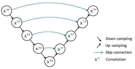
Figure 1.
U-Net network structure.
Although the solution to the feature loss problem was proposed by U-Net, the solution is too monolithic and still has flaws.
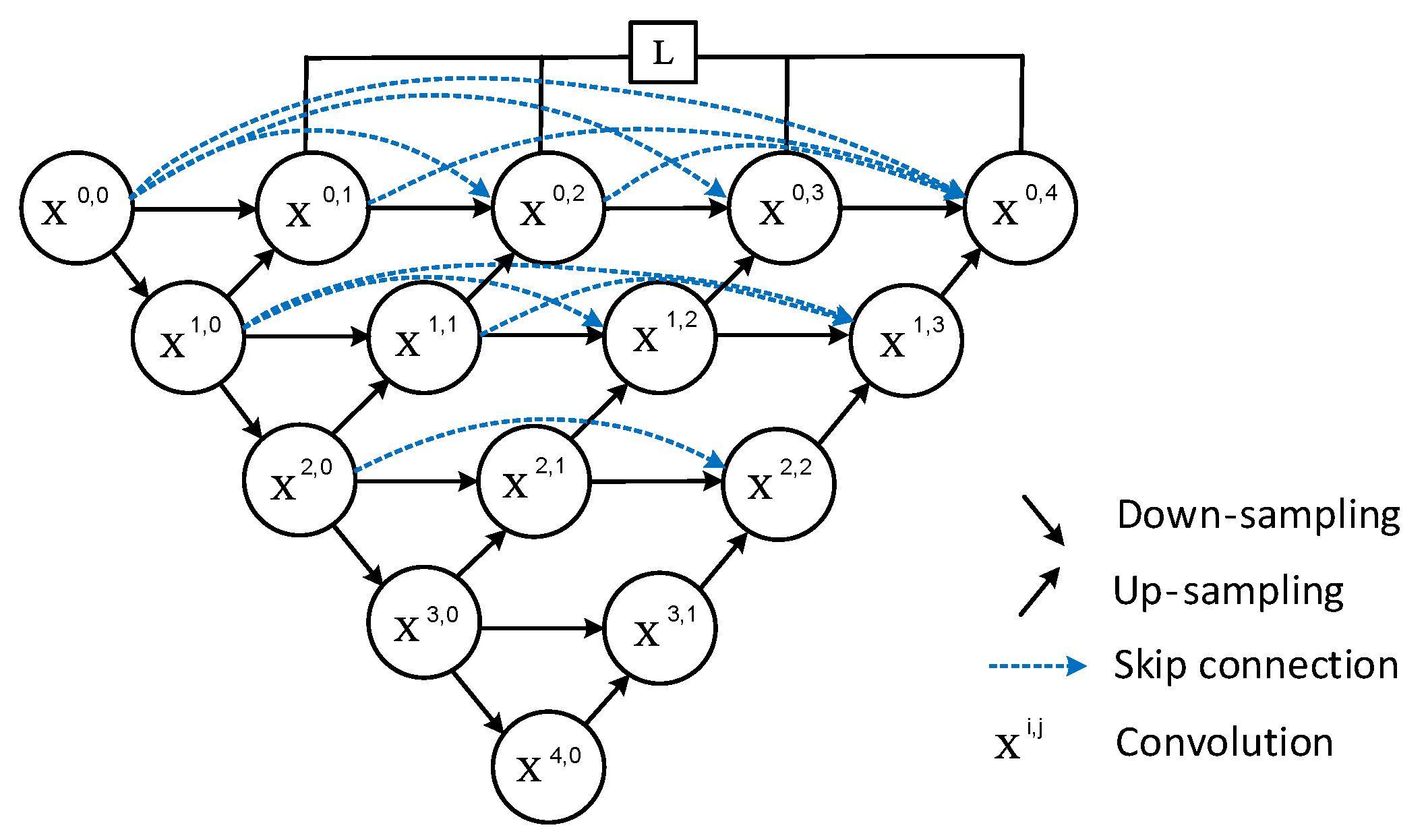
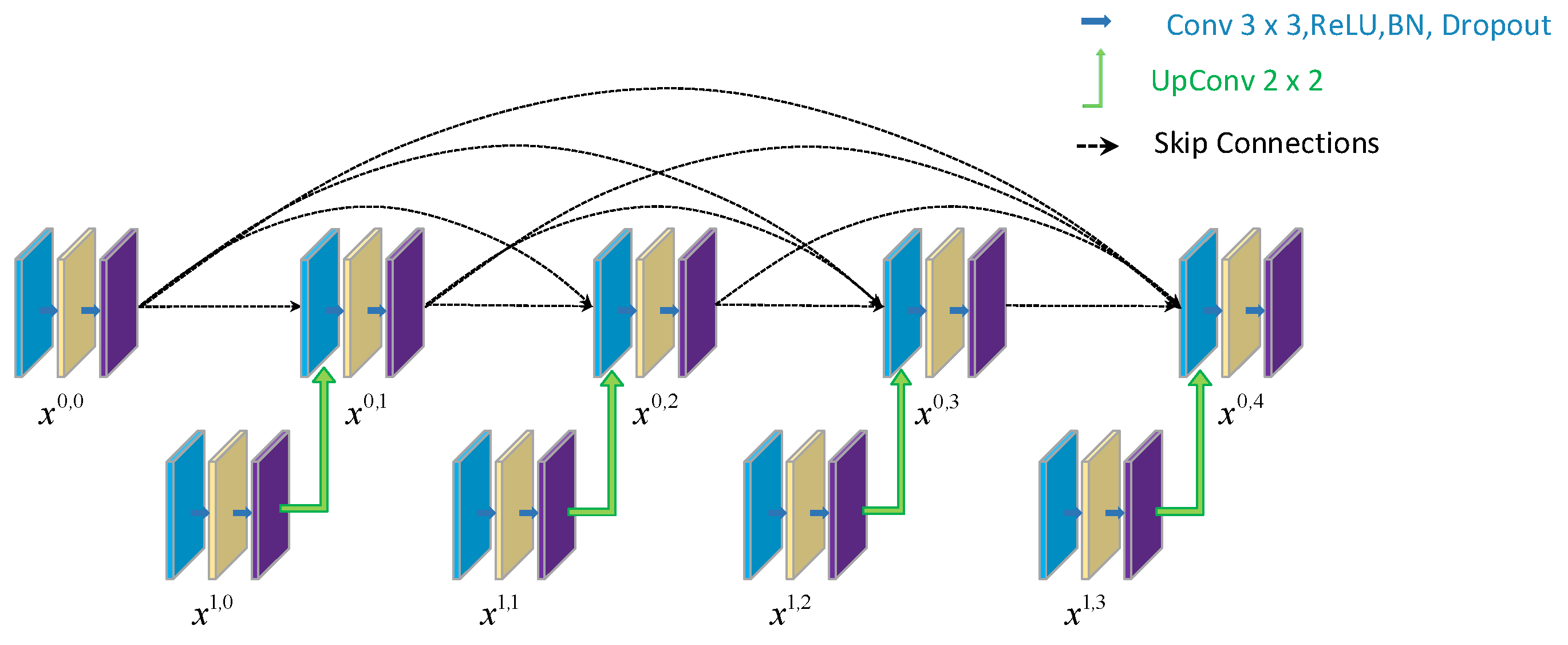
2.2. U-Net++
Due to the outstanding performance of U-Net in the field of segmentation, many improved algorithms based on U-Net have been proposed, such as U-Net++, which was proposed in 2018. Figure 2 shows the network structure of U-Net++. U-Net++ contains multiple U-Net structures. To minimize eigenvalue loss during upsampling and skip processes, the network employs dense downsampling and skip connections, thereby significantly enhancing segmentation performance.
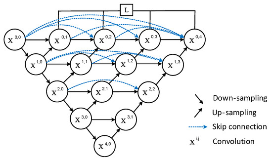
Figure 2.
U-Net++ network structure.
Although Unet++ has optimized some issues at present, the problem of feature loss still exists. Therefore, it is necessary to explore an effective method to deal with feature loss problems.
3. Methods
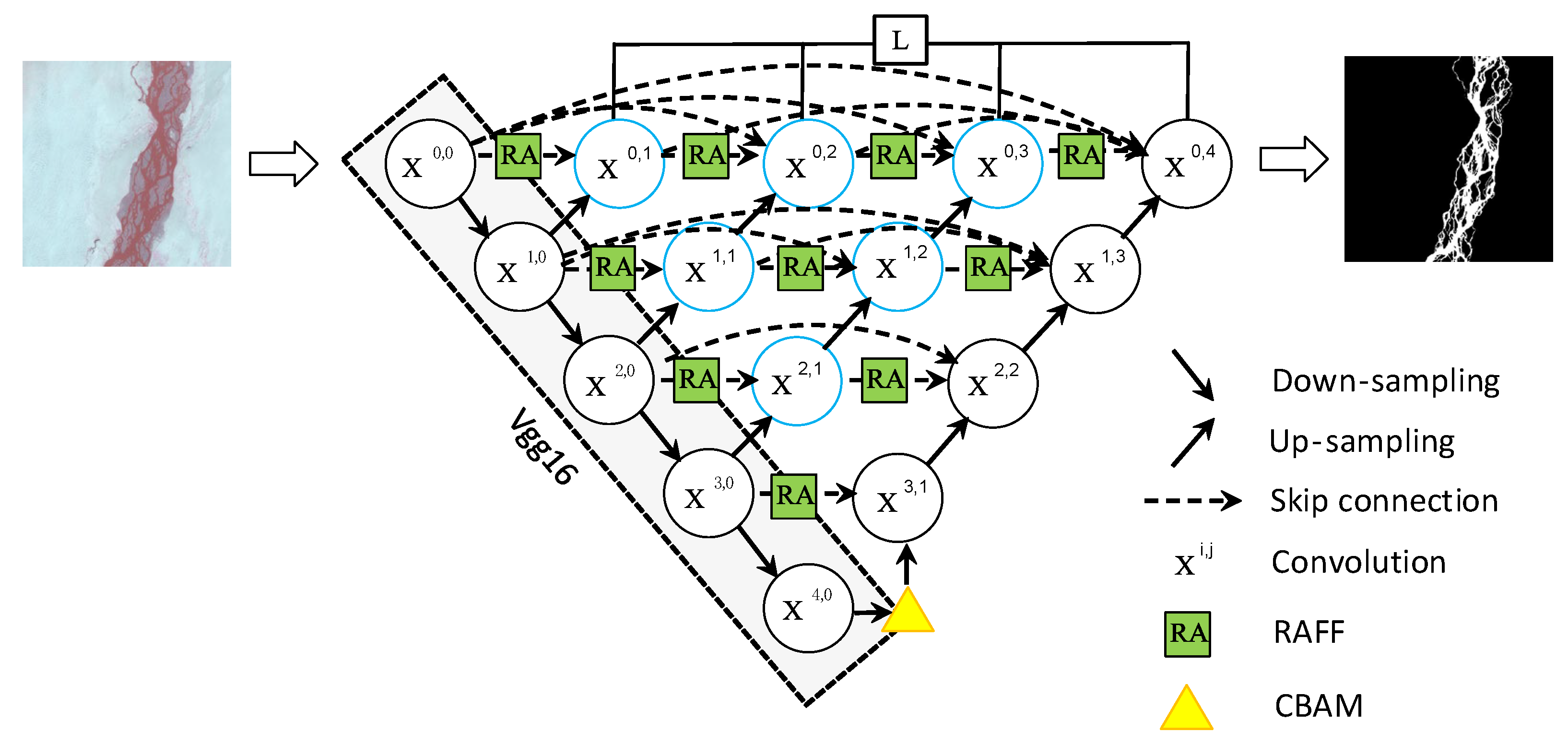
3.1. Overall Architecture
The river segmentation of remote sensing images in cold and arid areas is dichotomized [25]. In this paper, we explore a river extraction method for remote sensing images in cold and arid areas. The overall network structure is shown in Figure 3. The river attention U-shaped network (RAU-Net++) proposed in this paper uses the VGG16 structure as the backbone network, and in order to make the network pay more attention to the information of the fine river, an end-to-end encoder–CBAM-decoder network is designed by introducing the CBAM at the end of the encoder. Since the original U-Net only upsampled the end of the encoder, in order to optimize the problem of insufficient upsampling of the encoder, each convolutional layer of the encoder was up-sampled, and dense connections were introduced for each convolutional layer to learn the river features of different depths, and they were integrated by means of feature overlapping, which accomplished the deep interaction of different feature levels.

Figure 3.
The network structure of the method in this article.
In order to further optimize the dense connections, we introduce a residual attention feature fusion module (RAFF) at dense jump connections, which contains bottleneck attention-weighted branches, maximum pooling branches, and residual branches, which reduces the loss of information in each dense connection, and enables more edge detail features to be combined with the semantic information of the river channel, RAFF module optimizes the extraction of river edge detail information in remote sensing images, as well as to reduce the misdetection and omission of the river channel and its tributaries. Finally, the pixel-level optimization of river channel extraction in medium-resolution remote sensing images is carried out by combining the weighted loss function.
3.2. Feature Extraction
3.2.1. Backbone Network
Currently, VGG networks are widely used in semantic segmentation, target detection, and other computer vision tasks. The simplicity and superior robustness of the VGG16 network structure make it one of the classic models in the field of deep learning. The RAU-Net++ network proposed in this paper uses the first 13 layers of VGG16 as the backbone network for feature extraction of the river. The first 13 layers of VGG16 consist of 5 blocks, and the overall network structure is 2-2-3-3-3, which consists of 13 3 × 3 convolutional blocks (as shown in Table 2).
Table 2.
The first 13 layers of VGG16.
The input river image is a 564-channel false-color remote sensing image of 512 pixels × 512 pixels × 3. The convolution kernels in the 13 convolutional layers of VGG16 are all 3 × 3 in size, which can be divided into five groups of convolutional layers according to the number of channels. The convolutional layers and the maximum pooling layer downsampling stacking are used to extract the river channel features so as to expand the receptive field, in which the maximum pooling uses a 2 × 2 sized small pooling kernel; the activation function is Relu. The convolutional layers consist of five sets with channel numbers 64, 128, 256, 512, and 512, respectively. Through four rounds of downsampling, the input river remote sensing image is condensed into a 32 pixels × 32 pixels × 512 size output image, effectively capturing the essential features of the river in the remote sensing image.
3.2.2. CBAM Attention Network
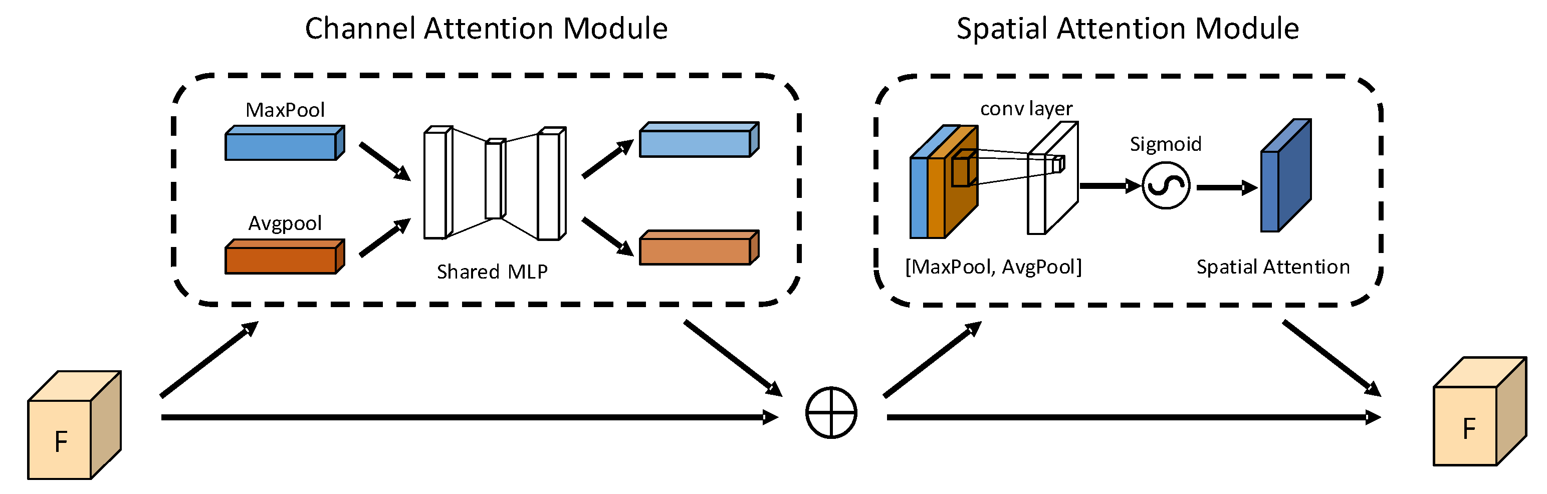
In deep learning, attention modules are commonly employed to focus on specific target features and suppress irrelevant features in the interference region, enhancing the model’s ability to prioritize relevant information. In the proposed model, we add a CBAM attention module at the end of the encoder to further supplement the learning of the mesh channel features of the river remote sensing image. CBAM consists of two sub-modules: the channel attention module (CAM) and the spatial attention module (SAM) (shown in Figure 4).

Figure 4.
CBAM attention module.
- Channel Attention Module
The feature maps are respectively input to two parallel maximum pooling layers and mean pooling layers, then the two results obtained by the multilayer perceptron machine () are sent to the fully connected layer operation and summed, and then the Sigmoid activation function generates the channel attention feature maps , and then multiply with the input again to obtain the adjusted feature maps () of the channel attention. and are computed as shown in Equations (1) and (2):
where is the Sigmoid activation function, denotes a multilayer perceptual machine with respective weights and , and denotes the average pooling operation and denotes the maximum pooling operation. is the input element in Equation (2).
- 2.
- Spatial Attention Module
With maximum pooling and mean pooling performed on F′ to obtain two feature maps and then the two are spliced, the convolution operation is performed to finally generate the spatial attention feature map , which is computed as shown in Equation (3). is multiplied with by element to obtain the final feature map , which is calculated as shown in Equation (4).
where is the sigmoid activation function and is the convolution kernel of size 7 × 7. Equation (4) takes the output of Equation (2) as input.
3.3. Feature Fusion
In the introduction of the backbone network, we utilized the initial 13 layers of 3 × 3 convolutional blocks from VGG16 to perform four rounds of downsampling on the original remote sensing image. However, each downsampling operation results in the loss of some detailed features. In contrast to the original Unet, which directly connects low-level detail features to high-level semantic features, our approach minimizes semantic discrepancies, thereby improving segmentation results. To solve this problem, it applies the dense jump connection of Unet++ to upsample each block of VGG16, respectively, aggregates the different semantic scales between the encoder and decoder through the dense jump connection, and adds the residual attention feature fusion module (RAFF) to the original Unet++’s dense jump connection. The RAFF module is located at the short jump connection, and the module’s complementary optimization of the dense jump connection has been complementarily optimized to enhance the extraction of fine stream information.
3.3.1. Dense Skip Connections
A dense jump connection consists of multiple standard convolutional modules and upsampling modules, which accumulate all the obtained feature maps and reach the final node through the dense convolutional blocks on the jump connection. This reduces the loss of detailed information from the encoder downsampling, makes the full combination between the low- and high-level information, realizes a deeper information interaction between the encoder and the decoder, and improves the feature utilization rate. (As shown in Figure 5).

Figure 5.
Dense skip connections.
Taking the first layer of the dense jump connection path as an example, one can see that there are three standard convolution modules between nodes and . Each standard convolutional module is connected to each other by a connectivity layer, which fuses the output of the standard convolutional module of the previous layer with the upsampling of the corresponding standard convolutional module of the next layer and, subsequently, combines the individual standard convolutional modules sequentially in the form of a cross-channel connection. The dense jump connection can be represented as Equation (5):
where denotes the output corresponding to this node, i denotes the index corresponding to the downsampling layer in sequence, and j denotes the index of the convolutional layer corresponding along the dense jump connectivity block. C(·) denotes the convolutional layer, and the convolutions are all followed by a Relu activation function. D(·) refers to the downsampling layer, U(·) refers to the upsampling layer, and [·] refers to the connectivity layer.
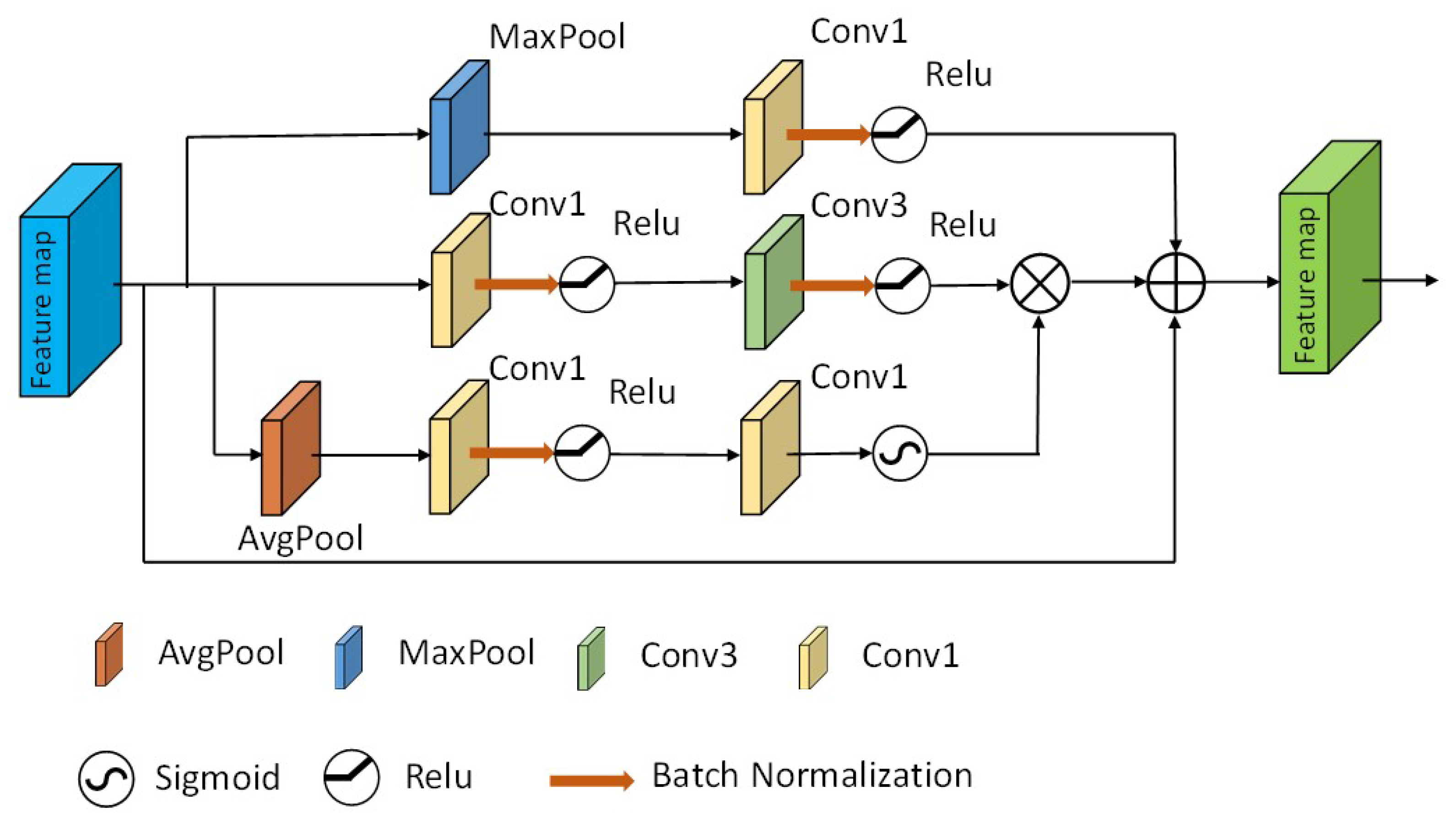
3.3.2. Residual Attention Feature Fusion Module (RAFF)
In this paper, the residual attention feature fusion module (RAFF) is proposed for the problems of easily missed detection of fine river branches and unrefined segmentation of river edges. The RAFF module is located at all the short jump connections, which is supplemented by optimizing the dense jump connections to make extracting the river edge information more adequate. It contains a bottleneck attention-weighted branch, maximum pooling branch, and residual branch (shown in Figure 6).

Figure 6.
RAFF module.
The bottleneck attention branch is composed of a parallel connection between the attention branch and the bottleneck branch. In the attention branch, we squeeze the input feature maps using average pooling. In order to increase the nonlinear expressiveness of the model to better fit the complex correlations between channels, we use two 1 × 1 convolutions for scaling between feature channels, respectively, perform batch normalization before the Relu activation function to improve the network generalization ability, and finally, use the Sigmoid activation function to map the feature vectors to a range between 0 and 1 to obtain a weight which provides a regional category overview of river remote sensing images. The attention branch automatically obtains the importance level of each feature channel by learning and then enhances the features of the river channel and suppresses the features except the river channel according to the importance level [32]. In the bottleneck branch, we use a 1 × 1 convolution and a 3 × 3 convolution, respectively, to integrate the information of the river features from the input feature maps to effectively extract the local river features and perform batch normalization and Relu activation after both convolution operations to retain more edge features for the river. Finally, the obtained attentional weights are multiplied channel-by-channel with the weights obtained through the bottleneck branch to obtain the output feature map.
Dense joins serve to adequately map the encoder features to the decoder, and in order to maximize the preservation of the river detail texture features during dense joins, we parallelize a maximum pooling branch with respect to the bottleneck attention-weighted branch. It consists of a maximal pooling layer with a pooling kernel of 3 × 3 size and a 1 × 1 convolution and, after convolution, a batch normalization and adding Relu activation function. Meanwhile, the maximum pooling branch in the first layer of short connections was concatenated with the downsampling in VGG16 to preserve more detailed texture features of the river.
In order to prevent excessive loss of river features, we introduced a residual branch relative to the other two branches in parallel to get the original features of the input image. Finally, we performed feature fusion of the three feature maps output from the three branches to obtain the final output feature map. The above process can be represented by Equation (6):
where is the input, denotes maximum pooling, denotes average pooling, denotes convolution kernel is 1 × 1 convolution, denotes convolution kernel is 3 × 3 convolution, and denotes computation, where is the batch normalization process, activation is performed after the batch normalization process, and denotes the Sigmoid computation.
3.4. Weighted Loss Function
A weighted loss function comprising cross-entropy (CE) loss, dice loss, focal loss, and Jaccard loss is employed.
Cross-entropy loss is a commonly used loss function for multicategorization tasks. Cross-entropy loss examines each pixel and compares the difference between the model predictions and the true labels.
The cross-entropy loss function for binary classification can be defined as Equation (7):
where is the total number of samples, and denotes the sample label, 1 for the positive class, and 0 for the negative class. denotes the probability that the sample is predicted to be a positive class after training.
In order to give more attention to hard-to-classify samples during the training process, focus loss uses a dynamic factor to adjust the weight of the difficult-to-classify and easy-to-classify samples based on the cross-entropy loss. When a sample is classified incorrectly, the probability of the correct category will be tiny, so the dynamic factor tends to 1, the loss does not change too much, and when the probability of the correct category is gradually increased tends to 1, the dynamic factor will tend to zero, indicating that the samples are easy to discriminate. Meanwhile, in the modulation factor, when γ is 0, the focus loss is equivalent to the cross-entropy loss, and the modulation factor will increase with γ. The formula makes the hard-to-classify samples in the model more focalized by using a function that measures the contribution of difficult-to-classify samples to the total loss.
Focal loss can be defined as Equation (8):
where is the dynamic factor, is the modulation factor added to cross-entropy loss, and the adjustable hyperparameter can be used to highlight the contribution of a few samples. We set the dynamic factor to the default value of 0.25 and the adjustable hyperparameter to the default value of 2 [33].
Dice loss is suitable for the scene of positive and negative sample imbalance. It can optimize the problem that the river occupies a small proportion in images, and the training focuses more on the mining of the river region. In contrast, the cross-entropy loss will deal with the positive and negative samples equitably, and when there is a small proportion of positive samples, it will be swamped by more negative samples.
The dice loss function can be defined as Equation (9):
where represents the total number of samples; is the label of the samples, with 1 for the positive class and 0 for the negative class, and is the predicted value.
Jaccard loss, also known as intersection over union (IoU) loss, is commonly used in semantic segmentation tasks to evaluate the similarity between the segmentation results of the model and the real segmentation labels and to measure the similarity and difference between two samples by calculating the degree of overlap between the two sets.
Jaccard loss can be defined as Equation (10):
where represents the total number of samples, denotes the label of the sample, and is the network prediction value.
We use a weighted combination of CE loss, dice loss, focal loss, and Jaccard loss, which can effectively segment the boundary of the river at the pixel level.
The final weighted loss is defined as follows:
where , , , and are the weight parameters of the four loss functions, respectively.
4. Experiments
4.1. Homemade Dataset
4.1.1. Experimental Area
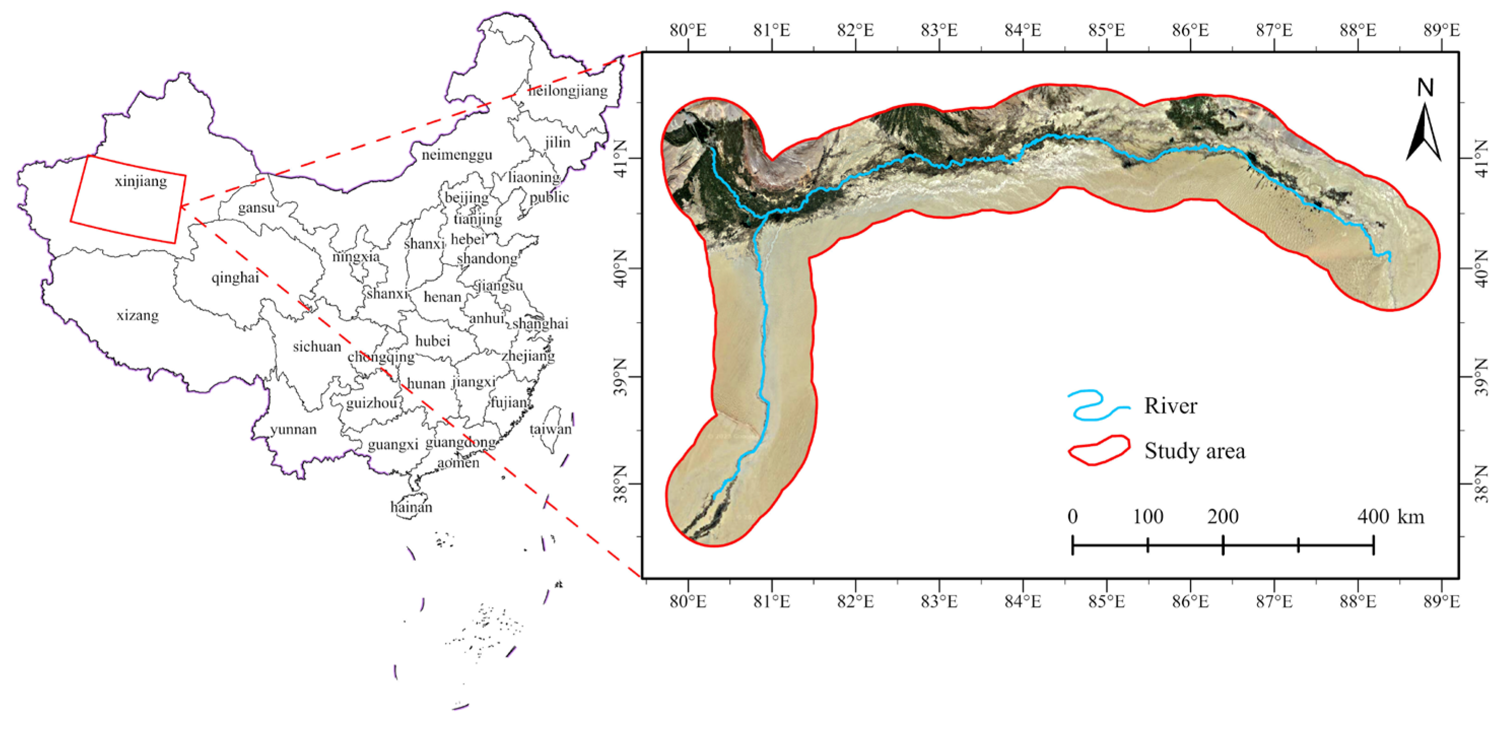
The research area of this paper is the Tarim River Basin (38°~42° N,80°~89° E), which is in an extreme arid desert climate. The Tarim River is the largest inland river in China [34], with a basin area of 198,000 square kilometers. The main object of the study is the mainstream of the Tarim River, mainly the Aksu River (72.0%) and the Hotan River (22.5%), and the total length of the mainstream of the river in the study area is 1321 km (shown in Figure 7).
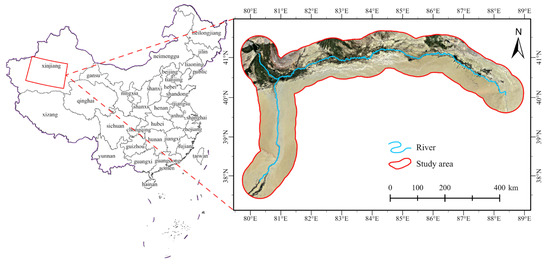
Figure 7.
Schematic diagram of experimental area.
4.1.2. Tarim River Mainstem Dataset
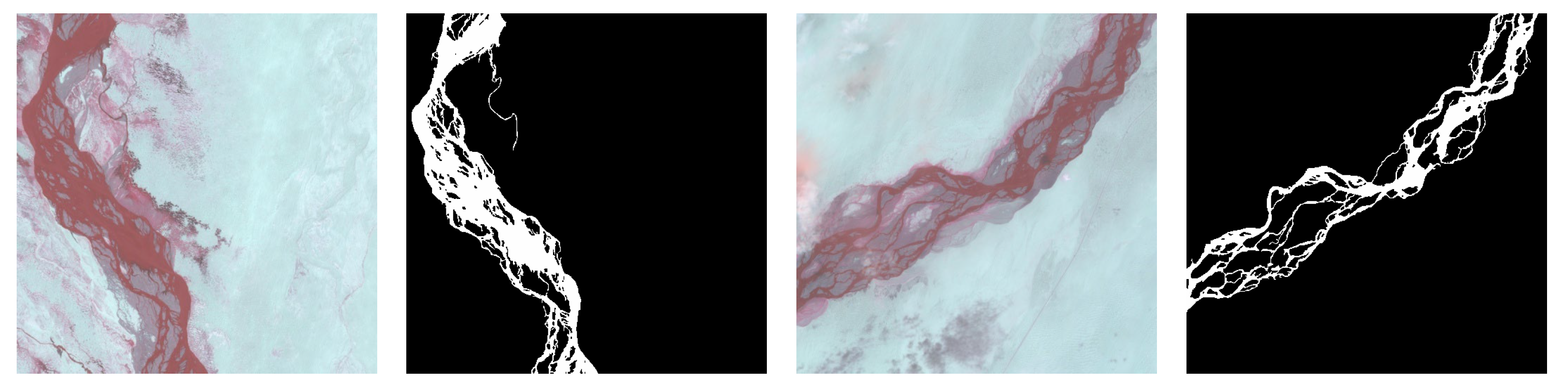
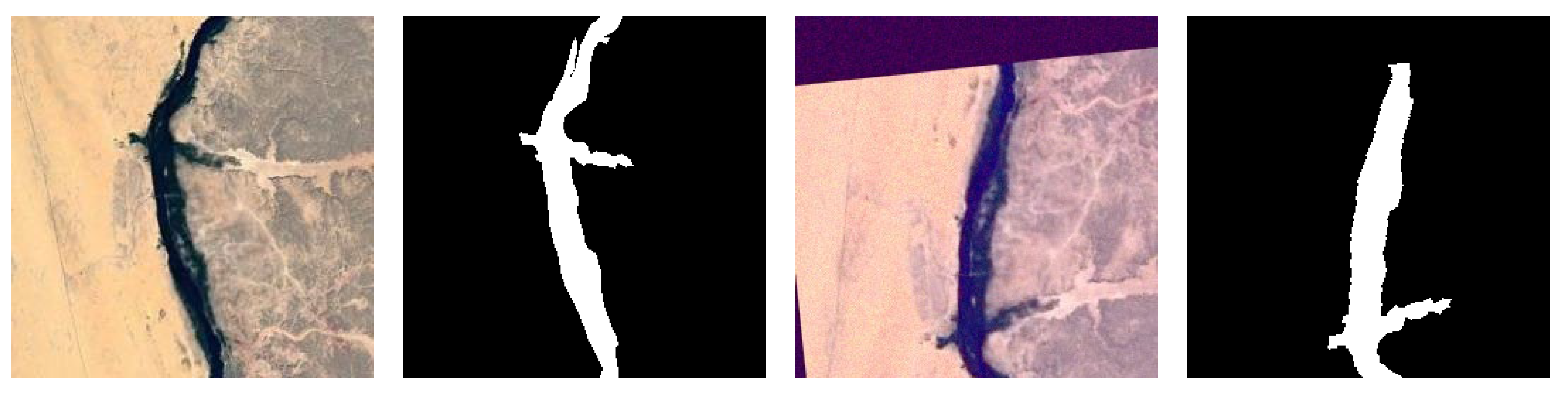
The dataset comes from the NASA Landsat8 satellite, which carries an OLI land imager, which includes nine bands with a spatial resolution of 30 m and an imaging width of 185 × 185 km. In this paper, we gathered data from six scenes within the Tarim River mainstream area. Considering the dichotomous nature of river segmentation, we opted for a combination of bands 5, 6, and 4 to enhance the differentiation between the river and background information. The resulting remote sensing image, synthesized from 564 bands, forms a non-standard false-color image by combining infrared and red bands. ENVI 5.3 and ArcMap 10.2 software were employed for remote sensing image processing and labeling. During the labeling process in ArcMap 10.2 software, the river was assigned a label of 255, while the non-river background was labeled as 0. After manually labeling the rivers in the six remote sensing image views, each view was randomly cropped into 400 512-pixel by 512-pixel river remote sensing image datasets containing the rivers, based on the location of the rivers. Finally, we selected 1900 datasets with a high proportion of rivers as the dataset. Some images in the dataset are shown in Figure 8. The dataset was then divided into training and validation sets with a 9:1 occupancy ratio.
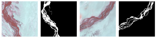
Figure 8.
Partial images and labels of the Tarim River mainstem dataset.
4.2. NWPU-RESISC45 Dataset
The NWPU-RESISC45 dataset is a dataset for remote sensing image scene classification (RESISC). It contains 31,500 RGB images of size 256 × 256 divided into 45 scene classes, each class containing 700 images. Among its notable features, RESISC45 contains varying spatial resolutions, ranging from 20 cm to more than 30 m/px. Around the theme of remote sensing river channels, we selected river scenes from 45 scenes, which contain 700 images, and used the Labelme tool to create corresponding labels. Some images in the dataset are shown in Figure 9. Finally, in order to correspond to the scale of the Tarim River dataset, we randomly expanded the original 700-image dataset using color change, brightness change, saturation change, color dithering, noise, rotation, scaling, translation, horizontal flip, vertical flip, and 90-degree rotation and finally obtained 1400 river remote sensing images as the validation dataset. The dataset was then divided into training and validation sets with a 9:1 occupancy ratio.
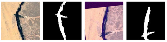
Figure 9.
Partial images and labels of the NWPU-RESISC45 dataset.
4.3. Experimental Setup
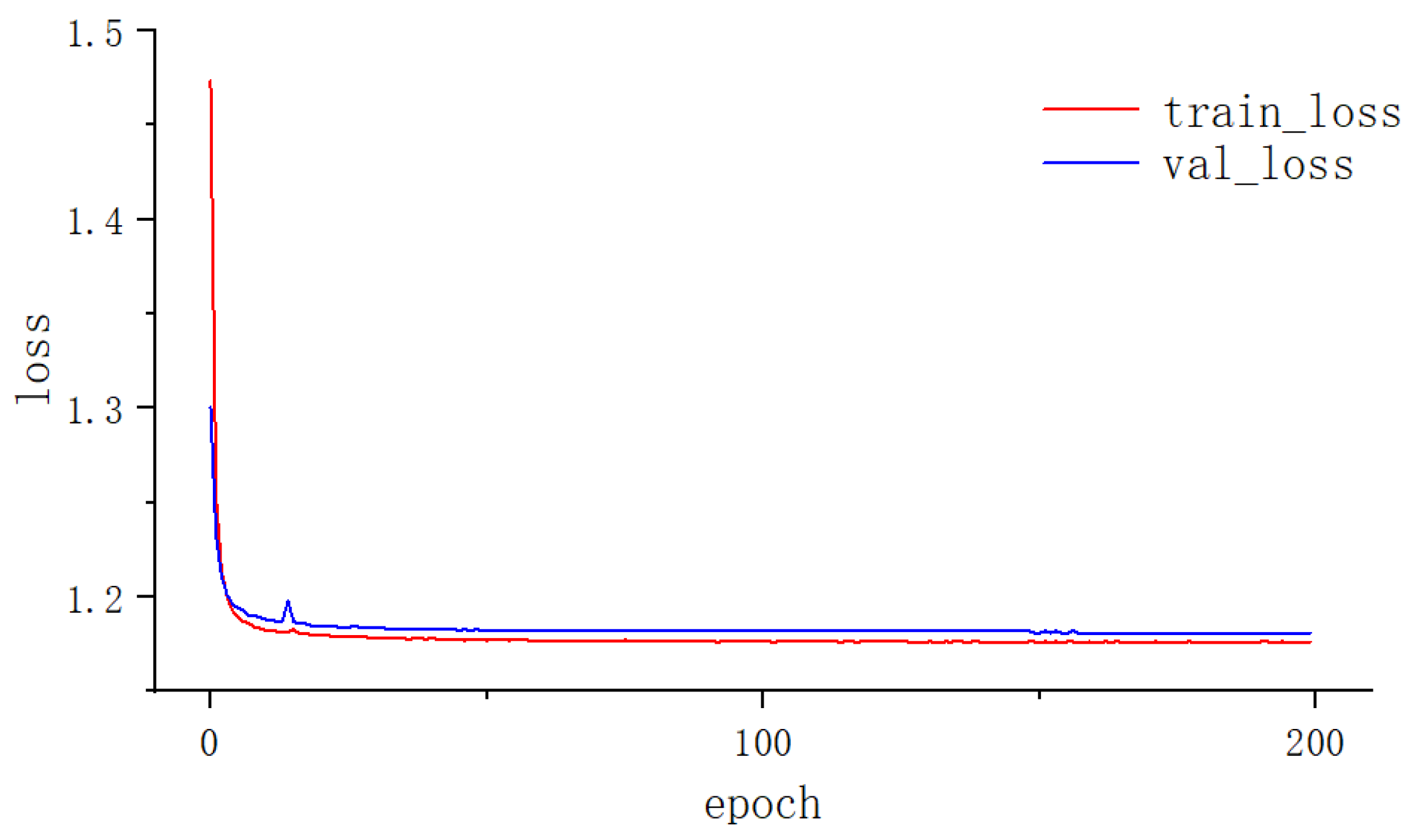
The experimental platform for this paper is an Ubuntu20 system, and the model code is implemented in Python 3.8 and Pytorch 1.12.0 environments. All models were trained and tested on a machine equipped with Intel(R) Xeon(R) Gold 5218R CPU 64 GB RAM (Intel Corporation, Santa Clara, CA, USA) and GeForce RTX 4090 GPU 24 GB (NVIDIA Corporation, Santa Clara, CA, USA) video memory. The batch size of the proposed model is 4, and the number of epochs for training is 200. The model optimizer is Adam, and the initial learning rate is fixed at 0.0001. In this paper, a weighted combination of the cross-entropy loss function, dice loss function, focus loss function, and Jaccard loss function is used. Figure 10 shows the loss curves of the model during the training and validation stages, where the training loss represents the error between the predicted results and the true values of the model’s training set, and the validation loss is the value calculated on the validation set by the loss function. In the training and validation phases, the loss curves converge quickly with the increase in cycles and there is no obvious oscillation, which indicates that the model effectively learns the river features from the remote sensing images and the model is not overfitted.
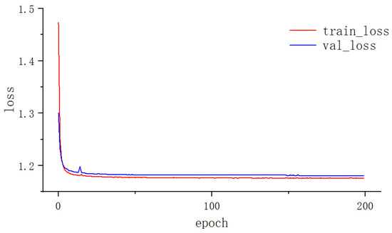
Figure 10.
The loss descent curves of the model.
4.4. Evaluation Metrics
We performed a quantitative evaluation between ground truth and predicted masked images in a pixel-by-pixel comparison using precision (P), F1 score, recall (R), ED, ED′, and intersection and integration ratio (IOU) as evaluation metrics. These metrics are commonly used for comprehensively evaluating binary river channel segmentation and assessing the accuracy of segmentation results. Among them, IOU is a metric that measures the accuracy of detecting the corresponding object in a given dataset. IOU can most intuitively and succinctly represent the effect of binary river channel segmentation in this paper. This metric is used to measure the correlation between the true and predicted values, and the higher the correlation, the higher the value [35]. To more intuitively and concisely depict the segmentation effectiveness in the experimental process of river channel extraction, this paper employs intersection and concurrency ratio values of the river category for evaluation testing during the experimental discussion comparing the mainstem and the CBAM module. Additionally, a series of experimental discussions are conducted using the IOU value as an index. For river segmentation extraction, the pixel distribution consists of the river and the background, with the pixels of the river set to 255 and the pixels of the background set to 0. There are four types of predictions: false positive (FP), false negative (FN), true positive (TP), and true negative (TN), respectively. FP indicates that the number of pixels of the river is incorrectly predicted (number of false positive samples). FN denotes the number of incorrectly predicted background pixels (number of false negative samples). TP denotes the number of correctly predicted river pixels (number of true positive samples). TN denotes the number of correctly predicted background pixels (number of true negative samples).
IOU, Precision, Recall, and F1 scores range between 0 and 1. When these metrics are used to assess segmentation accuracy, the score corresponding to the classification result for each pixel reflects the final segmentation effect. The higher the score, the better the accuracy of river segmentation. The segmentation quality will be easy to recognize when the accuracy and recall of the target are both higher than another target. For example, when the accuracy and recall are both 0.8, the segmentation quality is significantly higher than when the accuracy and recall are both 0.6. However, it is difficult to determine the segmentation quality when two metrics of one target are not simultaneously higher than the metrics of the other target. For instance, when the accuracy and recall of the two targets are (0.8, 0.8) and (0.9, 0.7), respectively. To deal with this problem, the precision and recall metrics can be combined into a single one, and here, a combination of ED and ED′ is used to capture the trade-off between the two metrics and give a clearer indication of segmentation quality [36]. Since the metric attribute values are close to 1, it is usually better to have a larger value for ED and a smaller value for ED′.
The river precision (P) is defined as Equation (12):
Recall (R) denotes the proportion of the river pixel segmentation that was predicted correctly, as shown in Equation (13):
The F1-score is the reconciled mean of the accuracy and is calculated as shown in Equation (14) as follows.
The intersection and merger ratio (IOU) denotes the ratio of the predicted intersection and concatenation, representing the true state of the river segmentation; the IOU is defined as Equation (15):
Through the Euclidean distance function, two distances are defined in the precision and recall metrics [37]. The first one, identified as ED, represents the distance to the point (0, 0) in space. The second one is labeled as ED′ and denotes the distance to (1, 1). As shown in Equations (16) and (17):
4.5. Experimental Results
4.5.1. Classic Network Comparison Experiment
The quantitative evaluation results are given in Table 3. It shows that the segmentation accuracy of U-Net++ and RAU-Net++ is higher than the other seven models. Among the nine models, RAU-Net++ obtains the highest IOU. The prediction accuracy is significantly improved by replacing the backbone network as well as improving the dense hopping connections compared to U-Net++; RAU-Net++ obtains 99.78%, 99.39%, 99.71%, and 99.75% for Precision, IOU, Recall, and F1 score, respectively. Since a larger value of ED or a smaller value of ED′ is better, both ED and ED′ of RAU-Net++ are optimal with values of 1.411 and 0.003, respectively. Compared with the other eight methods, the IOU increased by 30.7%, 16.06%, 14.4%, 13.71%, 5.82%, 3.67%, 2.81% and 0.55%, respectively.
Table 3.
Comparison results on the dataset of the mainstream of the Tarim River.
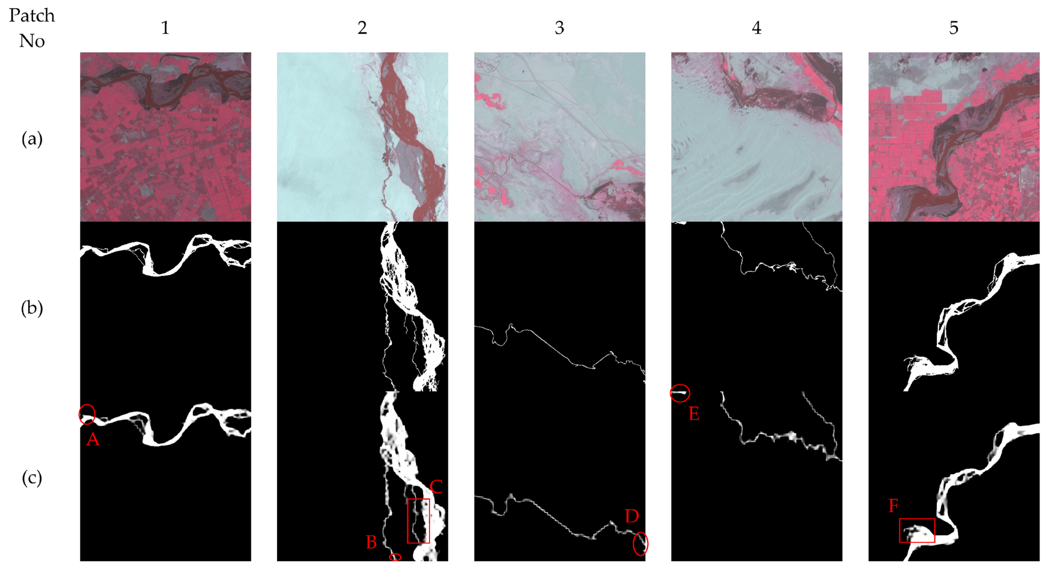
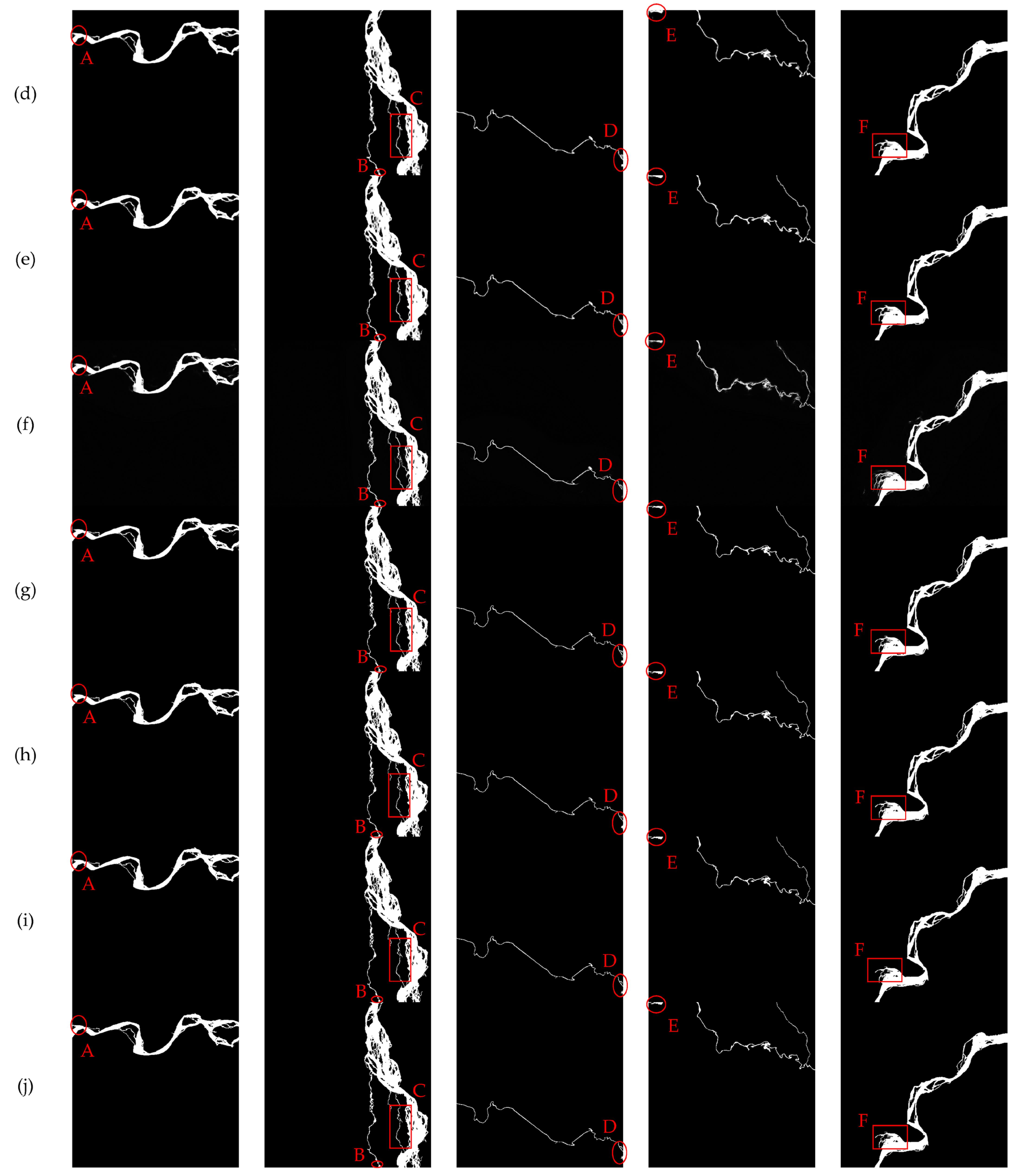
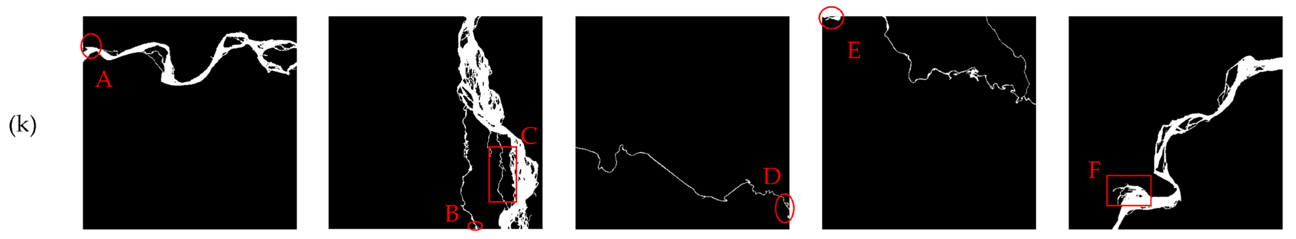
In order to compare the river channel extraction effect of various network models more intuitively, five remote sensing river images of 512 × 512 size are selected from the test data for demonstration and evaluation in this paper. Figure 9 shows the river channel extraction results of different networks. From top to bottom, the original remote sensing images, the original ground truth, and the PSPNet, Deeplabv3+, UperNet, MANet, TransUNet, LinkNet, U-Net, U-Net++, and RAU-Net++ are presented for the Prediction results. We use the image river dataset as the input image, and from the segmentation results of PSPNet, Deeplabv3+, UperNet, TransUNet, and LinkNet, the edges of the river cannot be segmented accurately, and there are many details missing. For instance, numerous river branches in designated area B cannot be finely segmented, leading to blurred and inaccurate segmentation edges. From the segmentation of U-Net, U-Net++, and RAU-Net++, the fineness of segmented river edges is significantly higher than that of the above five classical networks. Moreover, since U-Net uses ordinary jump connections for fusing multi-scale features, it leads to insufficient fusion of feature maps between the encoder and decoder, which makes the segmentation effect worse than that of U-Net++, which has dense jump connections. In addition, many mislabeled pixels were produced; for example, it is clear from the segmentation at C and F of MANet that a non-river branch was mis-detected as a river. Due to the optimized complementation of dense jump connections by the inclusion of the residual attention feature fusion module in RAU-Net++, RAU-Net++ is able to detect the regions that U-Net++ mis-detects and misses; for example, RAU-Net++ corrects the mis-detection as well as the omission of a river by U-Net++ in a small area at the marked regions A, B, D, and E. In Figure 11, by comparing the nine methods on five river remote sensing images, it can be seen that RAU-Net++ segmented the edges of the river channel finely and accurately, and retained satisfactory detailed features of the river channel.
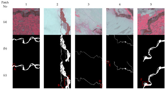
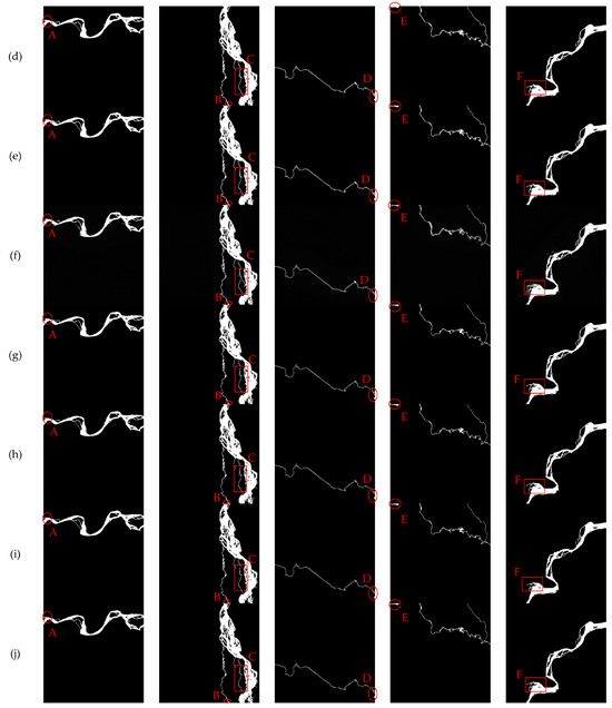
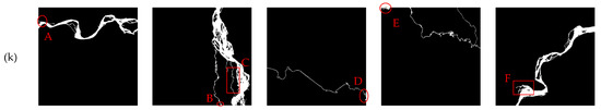
Figure 11.
Visualization results of several classical methods. (a) 5-6-4 band remote sensing images. (b) Ground truth. (c) PSPNet. (d) Deeplabv3+. (e) UperNet. (f) MANet. (g) TransUNet. (h) LinkNet. (i) U-Net. (j) U-Net++. (k) RAU-Net++.
4.5.2. Feature Extraction Network Comparison Experiments
In order to verify the superiority of the VGG16 backbone network in river segmentation in cold and arid areas, we compared it with the existing classical backbone networks and selected seven backbone networks, namely, VGG13 [28], VGG19 [28], ResNet50 [29], ResNext50 [38], DenseNet169 [39], EfficientNet-b5 [40], and Convnext [41], to conduct the backbone network comparison experiments (as shown in Table 4), in which we use the intersection and concurrency ratio, which can intuitively and succinctly reflect the river segmentation, as an evaluation index to compare the seven backbone networks for quantitative evaluation. Through Table 4, we can compare the IOU values and conclude that the VGG series has the best effect in river segmentation. The IOUs of VGG13, VGG16, and VGG19 are 98.84%, 98.89%, and 98.86%, respectively, and therefore, we choose VGG16 as the backbone network of RAU-Net++ to perform the river channel segmentation. Feature extraction and the results of feature extraction network comparison experiments are shown in Table 4.
Table 4.
Backbone network comparison experiments. The bolded section indicates optimal parameters.
4.5.3. RAFF Module Ablation Experiments
For both the maximum pooling branch and the bottleneck attention branch in the RAFF module, we conducted two experiments, one involving the removal of the maximum pooling branch and the other retaining it. Table 5 shows that the IOU is 99.18% after retaining the maximum pooling branch, which is 0.06% higher than the IOU when removing the maximum pooling branch. The experiments verify the effectiveness of the maximum pooling branch and prove the dominant role of the bottleneck attention branch in the RAFF module.
Table 5.
Maxpool branch ablation experiments.
4.5.4. Comparison Experiment of Adding Modules
In order to select the optimal attention module to optimize the feature extraction network, we carry out comparison experiments between the CBAM attention module and other classical attention modules at the upsampling of the end of the VGG16 backbone network based on the RAFF module after adding the RAFF module at the short jump connection. We select the four attention modules, SE [42], CA [43], RFB [44], and ULSAM [45], for comparison. The best effect is the CBAM module, with an IOU value of 99.20%. The results show that the effect of adding the CBAM attention module at the upsampling at the end of the backbone network is optimal. The results of the comparison experiments of the added modules are shown in Table 6.
Table 6.
Module comparison experiment. The bolded section indicates optimal parameters.
4.5.5. Loss Tuning Comparison Experiments
In this paper, a weighted loss function consisting of CE loss, dice loss, focal loss, and Jaccard loss is used. Firstly, the default parameter values of CE loss and dice loss are chosen; A and B are 1 and 2, respectively. The default values are verified to be the most optimal choice through the experiments in Table 7. Then, according to the determined A and B values, the focal loss parameter C is used for the tuning experiments, and the values are taken from 5 to 100 from low to high. The best results were obtained when C was 20, as can be seen in Table 8. Finally, according to the determined A, B, and C, the tuning experiments of Jaccard loss parameter D are carried out, and D is set to 0.1–1.5 from low to high, respectively. Table 9 shows that the network is optimal when D is 0.9. According to the three loss tuning comparison experiments, it can be concluded that the IOU improvement is the largest when A, B, C, and D are 1, 2, 20, and 0.9, respectively, which is 0.18% higher than the IOU of the corresponding network when the original CE loss and Dice loss are combined. The experiments proved that the final parameter combination results in the optimal choice.
Table 7.
Parameter adjustment experiment of CE loss and dice loss. The bolded section indicates optimal parameters.
Table 8.
Parameter adjustment experiment of focal loss. The bolded section indicates optimal parameters.
Table 9.
Parameter adjustment experiment of Jaccard loss. The bolded section indicates optimal parameters.
4.5.6. RAU-Net++ Network Ablation Experiments on Tarim River Mainstem Dataset
RAU-Net++ borrows the dense connectivity structure from Unet++. We can see from the results of the ablation experiment in Table 10 that U-Net++ containing dense connectivity improves the IOU by 2.27% compared to the original U-Net, 0.05% after replacing the backbone network with VGG16, and 0.29% after adding the RAFF module. When the CBAM attention module is added at the upsampling at the end of the encoder and no RAFF module is added, we find that its IOU is reduced by 0.13% compared to the original U-Net++. However, after adding the CBAM attention module on top of the RAFF module, the IOU is differently improved compared to the original U-Net++ network and the network with the RAFF module only, and the experimental results illustrate that the two differently positioned modules added to the RAU-Net++ network proposed in this paper have complementary effects and prove the holistic nature and effectiveness of the RAU-Net++ network. Finally, we perform the pixel-level optimization of river edge information extraction using the optimal combined weighted loss function after the IOU is improved by 0.19%.
Table 10.
Tarim river mainstem dataset overall network ablation experiments results. The bolded section indicates optimal parameters.
4.5.7. RAU-Net++ Network Ablation Experiments on NWPU-RESISC45 Dataset
Since the generalizability of the RAU-Net++ network cannot be verified by using only one Tarim River dataset, we used the river remote sensing dataset in the NWPU-RESISC45 dataset to perform ablation experiments as a way to verify the generalizability of the network. The results of the ablation experiments on NWPU-RESISC45 are shown in Table 11. From the experimental results, it can be seen that although the Recall of our proposed RAU-Net++ network decreases to 96.72%, the Precision reaches 98.21%, and its improvement compared to U-Net++ is 1.54%. Both ED and ED′ are optimal. The above experiments demonstrate the overall effectiveness and generalization of the proposed model in river remote sensing images.
Table 11.
NWPU-RESISC45 dataset overall network ablation experiments results. The bolded section indicates optimal parameters.
5. Conclusions
Building on the approach to finely segment the dynamic edges of perennially changing river channels and accurately extract information from variable fine river branches, we introduce RAU-Net++, a river channel extraction model for remote sensing imagery. Due to the false detection and missed detection of U-Net++ in small river channels, our model leverages VGG16 for river feature extraction and enhances expressiveness by integrating CBAM at the backbone network’s end and our custom RAFF module at dense skip connections. The application of a weighted loss function effectively reduces training errors. Finally, ablation experiments on two datasets confirm the overall effectiveness and generalization of the network. Comparative analyses demonstrate the model’s optimal performance, affirming its efficacy and superiority in enhancing segmentation. Furthermore, comprehensive validation through diverse network prediction graphs reinforces the model’s reliability.
In prospect, notwithstanding noteworthy strides in the field, persistent challenges endure in the domain of remote sensing river segmentation. At present, the ground resolution of satellite images is constantly improving, and in the future, research and analysis of higher-resolution remote sensing river images are needed. Secondly, the substantial temporal commitment entailed by manual annotation could be mitigated through the adoption of weakly supervised learning methodologies. This strategy entails harnessing annotated data to acquire unlabeled counterparts, thereby ameliorating the temporal and resource burdens associated with manual labeling. Additionally, owing to the network’s depth and parameter intricacies, computational demands mandate high-performance graphics processing units (GPUs). In ablation experiments, the model computation, complexity, and real-time performance for RAU-Net++ are shown in Table 12. Consequently, forthcoming initiatives will be directed towards the judicious optimization of model parameters, aiming to streamline computational processes and augment training efficiency without perceptibly compromising the precision of the network.
Table 12.
RAU-Net++ network parameters in ablation experiments.
Author Contributions
Conceptualization, Y.T. and J.Z.; Methodology, Y.T.; Software, Y.T.; Validation, Y.T., J.Z. and Z.J.; Formal analysis, Y.T.; Survey, Y.T.; Resources, Y.T.; Data management, Y.T.; First draft, Y.T.; Writing—comments and editing, Y.T.; Visualization, Y.T. and Y.L.; Supervision, J.Z. and Z.J.; Project Management, J.Z.; Financing acquisition, Y.T., J.Z., Z.J., Y.L. and P.H. All authors have read and agreed to the published version of the manuscript.
Funding
This research was funded by the Key Research and Development Program of Xinjiang Uygur Autonomous Region, grant number 2022B02038.
Institutional Review Board Statement
Not applicable.
Informed Consent Statement
Not applicable.
Data Availability Statement
Data are available on request from the authors. The data are not publicly available due to the requirements of laboratory policies or restrictions such as confidentiality agreements.
Conflicts of Interest
The authors declare no conflict of interest.
References
- Gong, W.; Wang, P.; Wang, S.; Zhou, Y.; Cao, K. Methods of water body extraction inboundary river based onGF-2 satellite remote sensing image of high resolution. J. Eng. Heilongjiang Univ. 2018, 9, 1–7. [Google Scholar]
- Liu, B.J.; He, L.Y.; Li, H.Y. Runoff Variation and Its Induced Factors of the Riverin Arid Area. Water Resour. Res. 2022, 40, 40–43. [Google Scholar]
- Feng, K.X. Research on River Extraction Method from Remote Sensing Image. Master’s Thesis, Changchun University, Changchun, China, 2020. [Google Scholar]
- Verma, U.; Chauhan, A.; Pai, M.M.M.; Pai, R. DeepRivWidth: Deep learning based semantic segmentation approach for river identification and width measurement in SAR images of Coastal Karnataka. Comput. Geosci. 2021, 154, 104805. [Google Scholar] [CrossRef]
- Wu, X.; Zheng, Y.; Wu, B.; Tian, Y.; Han, F.; Zheng, C. Optimizing conjunctive use of surface water and groundwater for irrigation to address human-nature water conflicts: A surrogate modeling approach. Agric. Water Manag. 2016, 163, 380–392. [Google Scholar] [CrossRef]
- Guo, B.; Zhang, J.; Li, X. River Extraction Method of Remote Sensing Image Based on Edge Feature Fusion. IEEE Access 2023, 11, 73340–73351. [Google Scholar] [CrossRef]
- Khurshid, M.H.; Khan, M.F. River extraction from high resolution satellite images. In Proceedings of the 2012 5th International Congress on Image and Signal Processing, Chongqing, China, 16–18 October 2012; pp. 697–700. [Google Scholar]
- Zhu, H.; Li, C.; Zhang, L.; Shen, J. River Channel Extraction from SAR Images by Combining Gray and Morphological Features. Circuits Syst. Signal Process 2015, 34, 2271–2286. [Google Scholar] [CrossRef]
- Yousefi, P.; Jalab, H.A.; Ibrahim, R.W.; Mohd Noor, N.F.; Ayub, M.N.; Gani, A. River segmentation using satellite image contextual information and Bayesian classifier. Imaging Sci. J. 2016, 64, 453–459. [Google Scholar] [CrossRef]
- Deepika, R.G.M.; Kapinaiah, V. Extraction of river from satellite images. In Proceedings of the 2017 2nd IEEE International Conference on Recent Trends in Electronics, Information & Communication Technology (RTEICT), Bangalore, India, 19–20 May 2017; pp. 226–230. [Google Scholar]
- Fu, J.; Yi, X.; Wang, G.; Mo, L.; Wu, P.; Kapula, K.E. Research on Ground Object Classification Method of High Resolution Remote-Sensing Images Based on Improved DeeplabV3. Sensors 2022, 22, 7477. [Google Scholar] [CrossRef]
- Li, Z.; Liu, F.; Yang, W.; Peng, S.; Zhou, J. A Survey of Convolutional Neural Networks: Analysis, Applications, and Prospects. IEEE Trans. Neural Netw. Learn. Syst. 2022, 33, 6999–7019. [Google Scholar] [CrossRef]
- Hughes, M.J.; Kennedy, R. High-Quality Cloud Masking of Landsat 8 Imagery Using Convolutional Neural Networks. Remote Sens. 2019, 11, 2591. [Google Scholar] [CrossRef]
- Yu, L.; Wang, Z.; Tian, S.; Ye, F.; Ding, J.; Kong, J. Convolutional Neural Networks for Water Body Extraction from Landsat Imagery. Int. J. Comput. Intell. Appl. 2017, 16, 1750001. [Google Scholar] [CrossRef]
- Shelhamer, E.; Long, J.; Darrell, T. Fully Convolutional Networks for Semantic Segmentation. IEEE Trans. Pattern Anal. Mach. Intell. 2017, 39, 640–651. [Google Scholar] [CrossRef] [PubMed]
- Kang, J.; Guan, H.; Peng, D.; Chen, Z. Multi-scale context extractor network for water-body extraction from high-resolution optical remotely sensed images. Int. J. Appl. Earth Obs. Geoinf. 2021, 103, 102499. [Google Scholar] [CrossRef]
- Ronneberger, O.; Fischer, P.; Brox, T. U-Net: Convolutional Networks for Biomedical Image Segmentation. In Proceedings of the Medical Image Computing and Computer-Assisted Intervention—MICCAI 2015, Cham, Switzerland, 5–9 October 2015; pp. 234–241. [Google Scholar]
- Chaurasia, A.; Culurciello, E. LinkNet: Exploiting Encoder Representations for Efficient Semantic Segmentation. arXiv 2017, arXiv:1707.03718. [Google Scholar]
- Zhao, H.; Shi, J.; Qi, X.; Wang, X.; Jia, J. Pyramid Scene Parsing Network. arXiv 2017, arXiv:1612.01105. [Google Scholar]
- Xiao, T.; Liu, Y.; Zhou, B.; Jiang, Y.; Sun, J. Unified Perceptual Parsing for Scene Understanding. arXiv 2018, arXiv:1807.10221. [Google Scholar]
- Chen, L.-C.; Zhu, Y.; Papandreou, G.; Schroff, F.; Adam, H. Encoder-Decoder with Atrous Separable Convolution for Semantic Image Segmentation. In Proceedings of the Computer Vision—ECCV 2018, Munich, Germany, 4–8 September 2018; pp. 833–851. [Google Scholar]
- Zhou, Z.; Rahman Siddiquee, M.M.; Tajbakhsh, N.; Liang, J. UNet++: A Nested U-Net Architecture for Medical Image Segmentation. In Proceedings of the Deep Learning in Medical Image Analysis and Multimodal Learning for Clinical Decision Support; Springer: Cham, Switzerland, 2018; pp. 3–11. [Google Scholar]
- Liang, J.; Sun, G.; Zhang, K.; Gool, L.V.; Timofte, R. Mutual Affine Network for Spatially Variant Kernel Estimation in Blind Image Super-Resolution. arXiv 2021, arXiv:2108.05302. [Google Scholar]
- Chen, J.; Lu, Y.; Yu, Q.; Luo, X.; Adeli, E.; Wang, Y.; Lu, L.; Yuille, A.L.; Zhou, Y. TransUNet: Transformers Make Strong Encoders for Medical Image Segmentation. arXiv 2021, arXiv:2102.04306. [Google Scholar]
- Wang, H.; Shen, Y.; Liang, L.; Yuan, Y.; Yan, Y.; Liu, G. River Extraction from Remote Sensing Images in Cold and Arid Regions Based on Attention Mechanisam. Wirel. Commun. Mob. Comput. 2022, 2022, 9410381. [Google Scholar]
- Wu, J.; Sun, D.; Wang, J.; Qiu, H.; Wang, R.; Liang, F. Surface River Extraction from Remote Sensing Images based on Improved U-Net. In Proceedings of the 2022 IEEE 25th International Conference on Computer Supported Cooperative Work in Design (CSCWD), Hangzhou, China, 4–6 May 2022; pp. 1004–1009. [Google Scholar]
- Fan, Z.; Hou, J.; Zang, Q.; Chen, Y.; Yan, F. River Segmentation of Remote Sensing Images Based on Composite Attention Network. Complexity 2022, 2022, 7750281. [Google Scholar] [CrossRef]
- Simonyan, K.; Zisserman, A. Very Deep Convolutional Networks for Large-Scale Image Recognition. arXiv 2014, arXiv:1409.1556. [Google Scholar]
- Kaiming, H.; Xiangyu, Z.; Shaoqing, R.; Jian, S. Deep Residual Learning for Image Recognition. arXiv 2015, arXiv:1512.03385. [Google Scholar]
- Xia, M.; Cui, Y.; Zhang, Y.; Xu, Y.; Liu, J.; Xu, Y. DAU-Net: A novel water areas segmentation structure for remote sensing image. Int. J. Remote Sens. 2021, 42, 2594–2621. [Google Scholar] [CrossRef]
- Woo, S.; Park, J.; Lee, J.-Y.; Kweon, I.S. CBAM: Convolutional Block Attention Module. arXiv 2018, arXiv:1807.06521. [Google Scholar]
- Xu, Z.; Lu, T. Patch SVDD (support vector data description)-based channel attention embedding and improvement of classifier. J. Intell. Fuzzy Syst. 2023, 45, 10323–10334. [Google Scholar] [CrossRef]
- Lin, T.Y.; Goyal, P.; Girshick, R.; He, K.; Dollár, P. Focal Loss for Dense Object Detection. IEEE Trans. Pattern Anal. Mach. Intell. 2020, 42, 318–327. [Google Scholar] [CrossRef] [PubMed]
- Xiao, J.; Jin, Z.-D.; Ding, H.; Wang, J.; Zhang, F. Geochemistry and solute sources of surface waters of the Tarim River Basin in the extreme arid region, NW Tibetan Plateau. J. Asian Earth Sci. 2012, 54–55, 162–173. [Google Scholar] [CrossRef]
- Lu, X.; Zhang, C.; Ye, Q.; Wang, C.; Yang, C.; Wang, Q. RSI-Mix: Data Augmentation Method for Remote Sensing Image Classification. In Proceedings of the 2022 7th International Conference on Intelligent Computing and Signal Processing (ICSP), Xi’an, China, 15–17 April 2022; pp. 1982–1985. [Google Scholar]
- Zhang, X.; Feng, X.; Xiao, P.; He, G.; Zhu, L. Segmentation quality evaluation using region-based precision and recall measures for remote sensing images. ISPRS J. Photogramm. Remote Sens. 2015, 102, 73–84. [Google Scholar] [CrossRef]
- Clinton, N.; Holt, A.; Scarborough, J.; Li, Y.; Gong, P. Accuracy assessment measures for object-based image segmentation goodness. Photogramm. Eng. Remote Sens. 2010, 76, 289–299. [Google Scholar] [CrossRef]
- Huang, G.; Liu, Z.; Maaten, L.v.d.; Weinberger, K.Q. Densely Connected Convolutional Networks. arXiv 2016, arXiv:1608.06993. [Google Scholar]
- Xie, S.; Girshick, R.; Dollár, P.; Tu, Z.; He, K. Aggregated Residual Transformations for Deep Neural Networks. arXiv 2016, arXiv:1611.05431. [Google Scholar]
- Tan, M.; Le, Q.V. EfficientNet: Rethinking Model Scaling for Convolutional Neural Networks. arXiv 2019, arXiv:1905.11946. [Google Scholar]
- Liu, Z.; Mao, H.; Wu, C.-Y.; Feichtenhofer, C.; Darrell, T.; Xie, S. A ConvNet for the 2020s. arXiv 2022, arXiv:2201.03545. [Google Scholar]
- Hu, J.; Shen, L.; Albanie, S.; Sun, G.; Wu, E. Squeeze-and-Excitation Networks. arXiv 2017, arXiv:1709.01507. [Google Scholar]
- Zhang, C.; Lin, G.; Liu, F.; Yao, R.; Shen, C. CANet: Class-Agnostic Segmentation Networks with Iterative Refinement and Attentive Few-Shot Learning. arXiv 2019, arXiv:1903.02351. [Google Scholar]
- Liu, S.; Huang, D.; Wang, Y. Receptive Field Block Net for Accurate and Fast Object Detection. arXiv 2017, arXiv:1711.07767. [Google Scholar]
- Saini, R.; Jha, N.K.; Das, B.; Mittal, S.; Mohan, C.K. ULSAM: Ultra-Lightweight Subspace Attention Module for Compact Convolutional Neural Networks. arXiv 2020, arXiv:2006.15102. [Google Scholar]

Disclaimer/Publisher’s Note: The statements, opinions and data contained in all publications are solely those of the individual author(s) and contributor(s) and not of MDPI and/or the editor(s). MDPI and/or the editor(s) disclaim responsibility for any injury to people or property resulting from any ideas, methods, instructions or products referred to in the content. |
© 2023 by the authors. Licensee MDPI, Basel, Switzerland. This article is an open access article distributed under the terms and conditions of the Creative Commons Attribution (CC BY) license (https://creativecommons.org/licenses/by/4.0/).