Abstract
This study analyzes the corrosion inhibition efficiency of sodium molybdate (SM) solution on weldment specimens in 1 M HCl, based on H2 bubbles detection. The detection of the bubbles produced by the corrosion process is achieved by a YOLOv4 deep learning algorithm. The results indicate that the corrosion rate is higher on the weld metal zone than on the base metal zone in the same solution, which might be attributed to the coarser grain of the weld metal zone and the stability of the produced oxide layer. The addition of sodium molybdate was discovered to boost the stability of the oxide layer, hence enhancing the specimens’ corrosion resistance. The overall inhibitory efficiency of the sodium molybdate solution was 59% for the weld metal (WM) (0.4 g/L), 52% for the heat-affected zone (HAZ) (0.2 g/L), and 37% for the base metal (BM) (0.2 g/L). The object detection algorithm models showed 97% for the mAP and 0.98 for recall. The minimum average bubble detected for the WM was 0.353 /mm2 at an SM concentration of 0.4 g/L, while the HAZ was 0.612 /mm2 at 0.2 g/L, and the BM was 1.055 /mm2 at 0.2 g/L. The results of the bubbles detection appeared to be consistent with the corrosion experiment outcomes obtained by the potentiodynamic polarization and hydrogen volume measurement tests. This experiment validates the distinctiveness of the different weld zones in terms of the inhibitor concentration required for successful corrosion prevention, as well as the potential of analyzing corrosion using machine learning algorithms for object detection.
1. Introduction
The application of corrosion inhibitors is among the most useful techniques to preserve the internal surface of steel structures, for example, tanks and pipelines, for facing corrosion, mainly in acidic environments. An acidic environment can cause various problems with metals, for example, stress corrosion cracking (SCC) in chloride-rich environments [1]. Increasing a tiny number of inhibitors without substantially varying the concentration of any corrosive agent can decrease and avoid the reaction of a metal to its environment. The benefits of inhibitors are that they reduce the level of corrosion between the corrosive agents and the surface of the metal by making a passive film on the metal surface and do not intervene in the mechanical properties of the material compared to other corrosion prevention techniques [2,3]. Organic materials have great prospects for maximizing their role in the field of engineering [4], including for modifying corrosion processes. Corrosion inhibitors can be produced from organic and non-organic compounds. The advantages of organic compounds are they are non-toxic, affordable, renewable, and easy to produce [5,6] but still need a lot of research to fully understand their performance and mechanism. On another side, non-organic inhibitors have already been studied and tested [7,8,9].
The weldment metal exhibits microstructural variations along the melted zone/weld metal (WM), heat-affected zone (HAZ), and base metal (BM) because of the welding parameters [10] and process itself [11], and it is also able to cause galvanic corrosion in steel [12]. Welding parameters significantly influence the welded joints’ quality, structural integrity, and mechanical properties. Variations in parameters, such as the current type and magnitude, voltage, travel speed, electrode specifications, and shielding gas composition, directly impact crucial aspects, like the penetration depth, heat input, bead geometry, and the distribution of residual stress [10,13,14,15]. Achieving optimal parameter settings is essential to attain the desired weld properties and prevent defects. Studies on shielding gas show the effects of the shielding gas content on the microstructure and toughness, underscoring the importance of precise parameter control in welding processes [16]. Differences in the microstructure, including the grain size and shape, impact the active–passive response of a corroded surface in a welded structure. For instance, a finer grain may result in a reduced localized corrosion rate but an increased rate of uniform corrosion [17]. The corrosion behavior of the HAZ region of welded X70 steel pipes in naturally aerated solutions containing 0.5 M bicarbonate and 0.01 M chloride at an atmospheric temperature of 25 °C have been investigated by Khalaj et al. [18]. They found that the bainitic microstructure generated in the area that experiences fast cooling rates and high temperatures during welding such as the coarse grain HAZ (CGHAZ) and partially melted zone (PMZ) was easy to corrode as showed by their higher current density, whereas the weld metal region had the lowest corrosion current density.
Several investigations within welding research have underscored the presence of solid phase transitions that notably affect stress modifications during welding [19,20,21,22]. This transition commonly aligns with changes in mechanical characteristics, volumetric expansion, and Transformation-Induced Plasticity (TRIP). These modifications deeply impact the formation of residual stresses, prompting a recent focus on incorporating the effects of microstructure transformation into both experimental and simulated thermal–mechanical models for welding [23,24,25,26].
The mechanical properties of each weldment zone are significantly influenced by hydrogen, with the hydrogen diffusion behavior variance and stress field distribution in each phase being crucial factors impacting hydrogen embrittlement behavior [27]. Hydrogen atoms exhibit a tendency to diffuse and accumulate around imperfections in the crystal lattice, leading to elevated hydrogen pressure [28,29]. This process reduces the bond energy [30,31] and aids in the accumulation of dislocations or localized plastic deformation [32,33].
The main purpose of the inhibitor is to control hydrogen evolution and corrosion. This is performed when the reaction with the metal is taking place and the water decomposition process occurs [34,35]. The inhibitor must assist in the recombination of hydrogen gas and inhibit the penetration of hydrogen into the metal lattice to avoid embrittlement [36]. The detection of hydrogen gas produced during the corrosion inhibition process could be used as an indication of inhibitor performance [37].
Standard electrochemical test methods such as potentiodynamic polarization (PP) can be applied to determine inhibitor effectiveness in corrosion inhibition tests [38]. To gain more insight into inhibitor effectiveness, a combination approach can be performed using the detection of hydrogen gas (H2 bubbles) with these electrochemical methods and the bubble detection. This approach is able to provide more information on the effectiveness of an inhibitor.
Image extraction of the corrosion process could be performed through a polarization test, based on video acquisition. Each image provides insight into the metal surface material transformation process and the H2 bubbles’ spread [34,38]. Detecting the H2 bubbles at a certain corrosion rate condition is not an easy job, for instance, in scenarios characterized by low current density [34,39,40]. To detect bubbles from a corrosion process in a metal weldment image, a machine learning algorithm (GLCM/SVM method) was implemented [6]. In the deep learning concept, the computer will attempt to map a feature from a set of images through a training process to acquire certain patterns, for example, object sizes, color channels, and so on, to support object detection schemes [41,42]. Presently, a promising technology for object detection is YOLO (You Only Look Once), which has several parameters for justification, including the resulting model size, detection speed, and detection accuracy [43]. This algorithm is one of the popular object detections that has advantages in real-time performance and must be implemented with a training process on image data with the expected object class [44,45]. The computation of these algorithms can be run by utilizing the computer’s main processing tools or with the help of a graphics card to generate models for object detection. After the bubble is detected by the algorithm, the bubble can be quantified based on the weldment zones (weld metal, heat-affected zone, and base metal). Machine learning algorithms have been involved in the study of corrosion and inhibitors, such as quantum chemical variables [46], the molecular dynamics of the inhibitors [47], and measuring the immersion time and corrosion rate [48].
The purpose of this work is to detect bubbles produced from the corrosion inhibition process of a sodium molybdate on carbon steel based on H2 evolution using a deep learning approach. The integration of conventional electrochemical testing and advanced deep learning algorithms in this research is a novel approach that has the potential to improve the field. This novel combination not only enhances the accuracy of the results but also opens up new avenues for further research and discovery. By calculating the corrosion rate based on PP tests on carbon steel specimens in 1 M HCl solution with up to 0.4 g/L sodium molybdate and detecting bubbles with a deep learning method on hydrogen gas bubble images captured during the electrochemical test, this work reveals some fundamental aspects of the inhibition mechanism and provides an example of the usefulness of deep learning in corrosion inhibitor research.
2. Materials and Methods
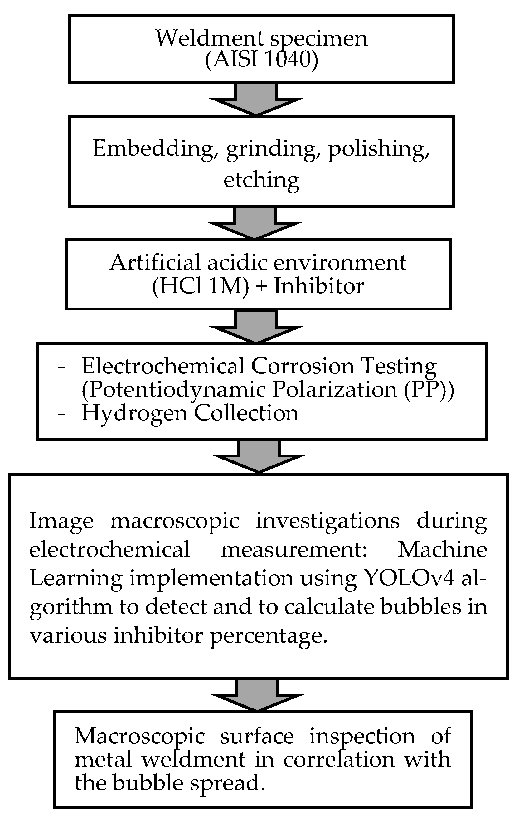
The process flowchart of the research framework is provided in Figure 1.
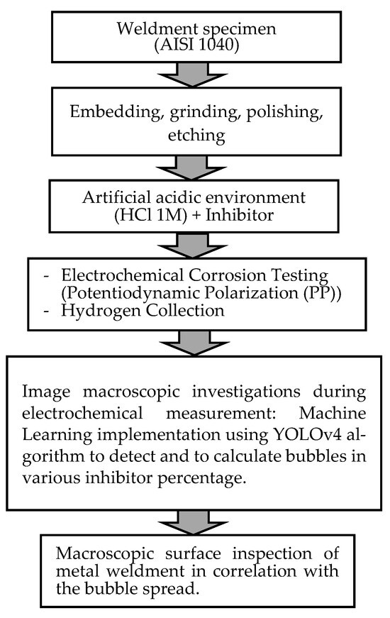
Figure 1.
Process flowchart of research framework.
2.1. Weldment Preparation
The weldment specimen was prepared using a Shielded Metal Arc Welding (SMAW) technique and E6013-type electrodes on AISI 1040 carbon steel plates (0.38 wt% C and 0.6 wt% Mn). The AWS A5.1 standard was employed [49], where the plate thickness is 8 mm. The SMAW technique was carried out due to its versatility and effectiveness in welding thicker steel plates, which is crucial for this project’s structural requirements. Its ability to penetrate and create strong, reliable welds on heavy materials, along with its adaptability to various environmental conditions, made it the optimal choice for ensuring the robustness and durability of the welded joints in this specific construction. The welding parameters are listed in Table 1.

Table 1.
SMAW process parameters.
2.2. Electrochemical Corrosion Testing
The corrosion testing methods for the specimens included hydrogen collection measurement, electrochemical testing, and hydrogen bubble detection. The specimens for the corrosion testing were divided into two types. The first type was cut from the weldment samples at the three zones of interest and ground with abrasive papers up to 2000 grit, and the second type used resin and was mounted in a container for electrochemical testing and recorded for video. The first type was applied to hydrogen collection and electrochemical testing and the second type targeted hydrogen bubble quantification.
Sodium molybdate (Na2MoO4) in powder form (22.3 wt% Na, 46.6 wt % Mo, and O 31.1 wt %) was dissolved into a 1 M HCL electrolyte solution. The solution will act as a corrosion test solution with varying concentrations of 0 g/L, 0.1 g/L, 0.2 g/L, 0.3 g/L, and 0.4 g/L.
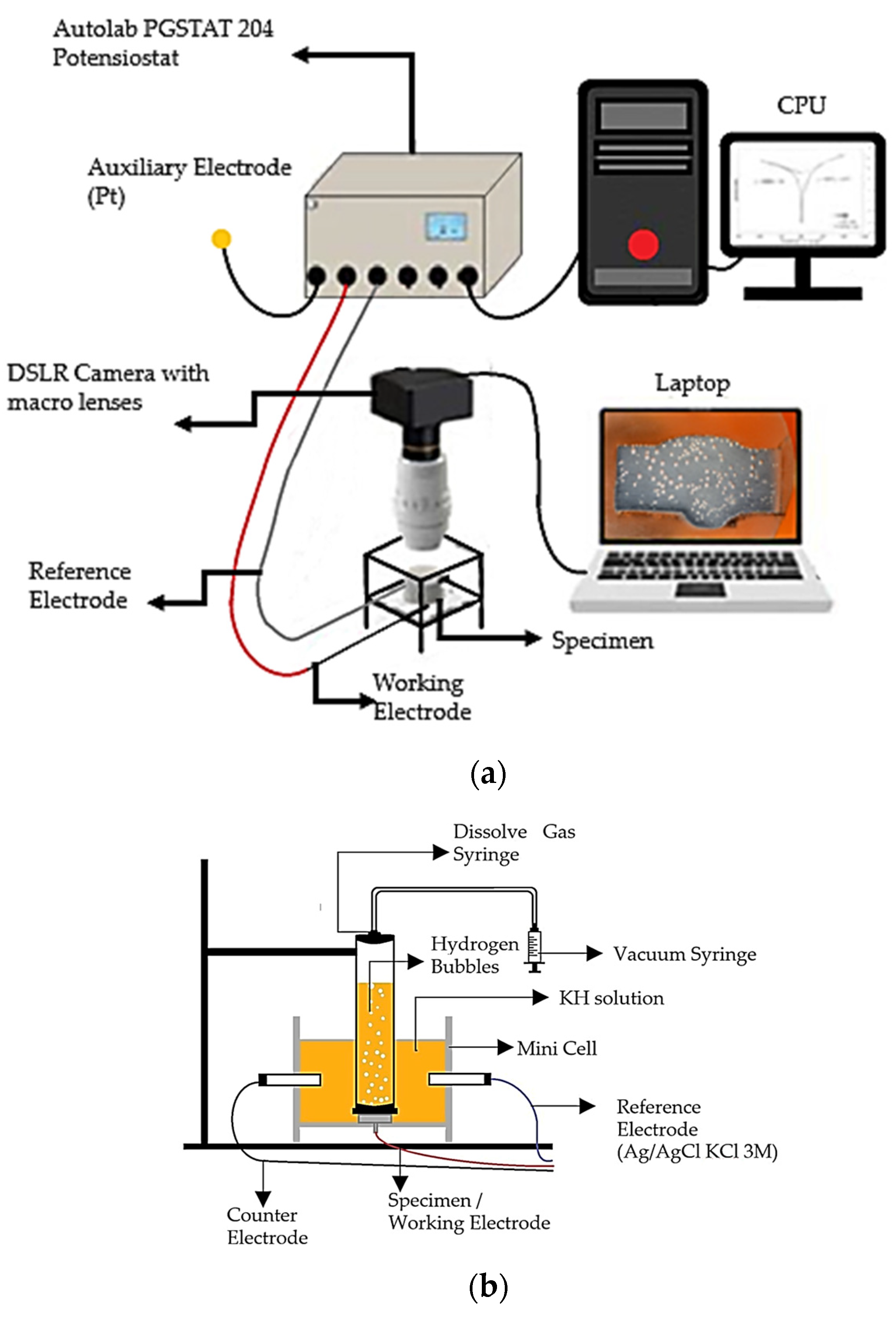
A range of corrosion testing solutions were prepared with various percentages of sodium molybdate, Na2MoO4 inhibitors, i.e., 0.1, 0.2, 0.3, and 0.4 g/L, into 1 M HCl. The electrochemical test methods were performed by potentiodynamic polarization with an Autolab potentiostat (PGSTAT 128N, Herisau, Switzerland). A three-electrode system was used for conducting the PP test, with the weldment specimen as the working electrode as shown in Figure 2a. The reference electrode was Ag/AgCl (3 M KCl), and the counter electrode was platinum. The PP test was measured at +/− 1 V from the corrosion potential (Ecorr) at a scan rate of 1 mV/s. Then, the Tafel plot extrapolation was analyzed by using the software tool associated with the potentiostat NOVA 1.11.

Figure 2.
Schematic illustration of (a) electrochemical data and video acquisition set-up and (b) H2 volume measurement set-up [6].
The inhibition efficiency IE (%) of the inhibitor was calculated by using the equation below:
where icorr(inh) and icorr are the corrosion current densities with and without the inhibitor, obtained by the extrapolation of the Tafel lines to the corrosion potential from the PP test.
Figure 2b shows the minicell was linked to the three-electrode cell within the solutions contained in the specimen container [6]. After closure, it was directed toward a 50 mL syringe designed for dissolved gas analysis (DGA) (Figure 2b), as well as to the solutions. This configuration was employed to quantify the volume of H2 gas generated during the PP test.
Three techniques—potentiodynamic polarization, hydrogen volume measurement, and deep learning—were employed using five specimens. Each test specimen underwent evaluation in distinct types of HCl solutions: HCl + SM 0 g/L, SM 0.1 g/L, HCl + SM 0.2 g/L, HCl + SM 0.3 g/L, and HCl + SM 0.4 g/L. Additionally, each specimen underwent five repetitions for the respective tests.
2.3. YOLOv4
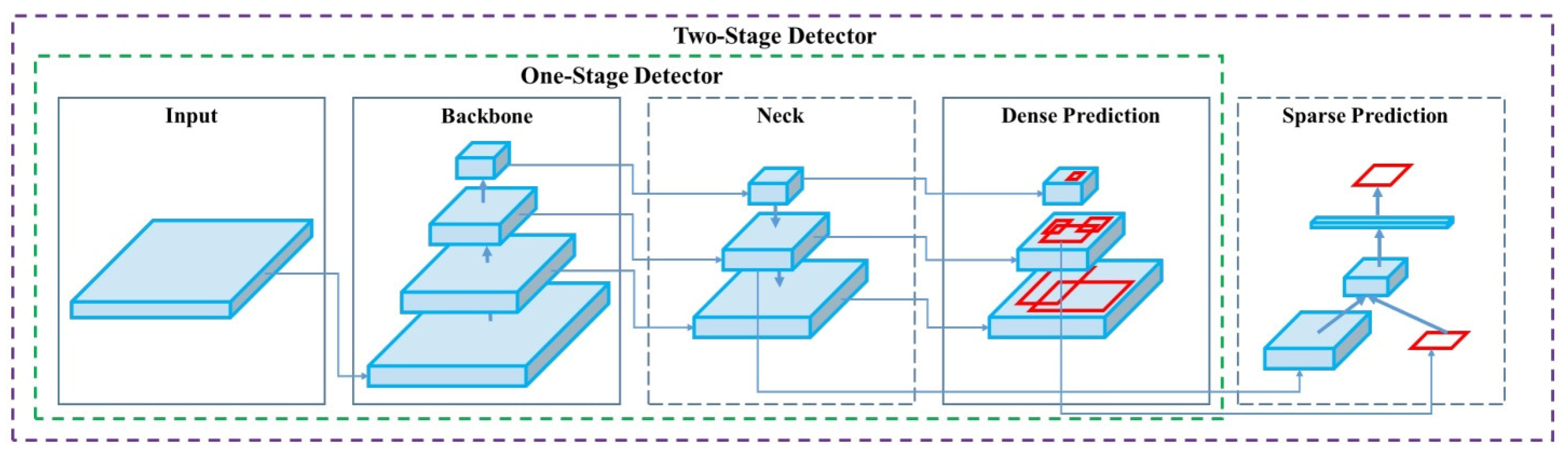
This study utilizes YOLOv4, an advanced version of the YOLO (You Only Look Once) object detection model, originally introduced by Redmon et al. [43]. YOLOv4, developed by Alexey Bochkovskiy, represents the fourth generation and significantly improves both the speed and accuracy compared to its predecessor, YOLOv3. YOLOv4 consists of three main components, the CSP-Darknet53 backbone, SPP Block, and PANet, and the detection head. The CSP-Darknet53 integrates CSP-DenseNet to enhance the operational speed, addressing the limitations of the previous versions. Various techniques are employed to optimize its performance, the structure of YOLOv4 can be shown in Figure 3. CutMix and Mosaic are the data augmentation methods. CutMix removes objects from training images and replaces them with objects from other images, while Mosaic combines four images into one, reducing the mini-batch size [50]. DropBlock acts as a regularization technique, preventing overfitting by excluding specific regions of the feature map during training. Class Label Smoothing ensures label normalization by allowing label values to range between 0 and 1, enhancing model robustness [51].
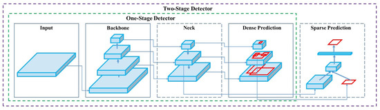
Figure 3.
The structure of YOLOv4 [40].
The input for this research consists of 3755 image datasets of bubbles. Yolomark was used for labeling and annotation. The output of YOLOv4 is a weights file that records the model’s ability to detect bubbles in a video or image.
Bag-of-Specials (BoSs) techniques in YOLOv4′s detector include the Mish activation function, SPP, SAM, PAN, and DioU-NMS [45]. Mish maintains a non-vanishing gradient, promoting smoother optimization, and serves as a regularizer by bounding negative outputs [52]. SPP ensures consistent output sizes regardless of varying feature map sizes, utilizing multi-filter pooling to preserve important contextual features [53]. SAM conveys spatial-wise information efficiently [54], and PANet transfers information between different levels, improving the localization accuracy [55]. DioU-NMS, the post-processing technique, uses Intersection over Union (IoU) for loss calculation, considering both the overlap and distance between predicted and actual bounding boxes. NMS is applied to remove overlapping bounding boxes, retaining only highly reliable ones [56].
These YOLOv4 components contribute to enhanced performance, efficient computation, accurate localization, and reliable post-processing, making it a powerful tool for object detection in various applications. This study utilizes this advanced model to detect bubbles on the surface of welding metal, demonstrating the effectiveness and versatility of YOLOv4 in real-world scenarios.
In this study, for the bubble detection method, the multi-object-based detection strategy was applied. The dataset was taken through digital camera acquisition and a macro lens. It consists of 3755 images of bubbles, which are divided into 80% for training and 20% for testing.
Figure 4a shows two different conditions for the same welding metal, before and after corrosion. Before corrosion, the metal surface looked relatively homogenous and there were no visible boundaries between the weld metal, heat-affected zone, and base metal. Figure 4b shows an example of a common polarization curve and the timestamp of the video acquisition. The video data were taken for 10 min using a digital camera (DSLR) and a macro lens with 3.2× magnification, which produced a size of 1280 × 720 pixels and 50 fps. Each image has a size ranging from 1 to 2 MB. The size of the image for the data training resulting from the acquisition process is 352 × 352 pixels, with sizes ranging from 100 to 300 KB. For labeling, annotation was accomplished by using YOLOmark [57], labeling in YOLOv4 by marking objects with box-shaped delimiters and adjusting the width and height of the object. The data label format in YOLOv4 has the extension .txt. A data analysis for bubble detection was performed using the images captured within a 6 to 10 min timeframe with a consideration to ensure good image clarity.
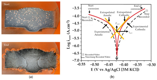
Figure 4.
(a) Example image of bubbles in metal weldment: start and end of corrosion process, and (b) video acquisition timestamp on common potentiodynamic polarization curve [6].
Model training and testing employed an AMD Ryzen 7 5800H with 16 GB RAM. The operating system was Windows 11 with a single NVIDIA GeForce RTX 3060 6 GB GPU RAM, which was considered sufficient for training and testing in this study. The setting model configuration of YOLOv4 is shown in Table 2.
Table 2.
Model configuration of YOLOv4.
3. Results and Discussion
3.1. Weldment Structures and Hardness
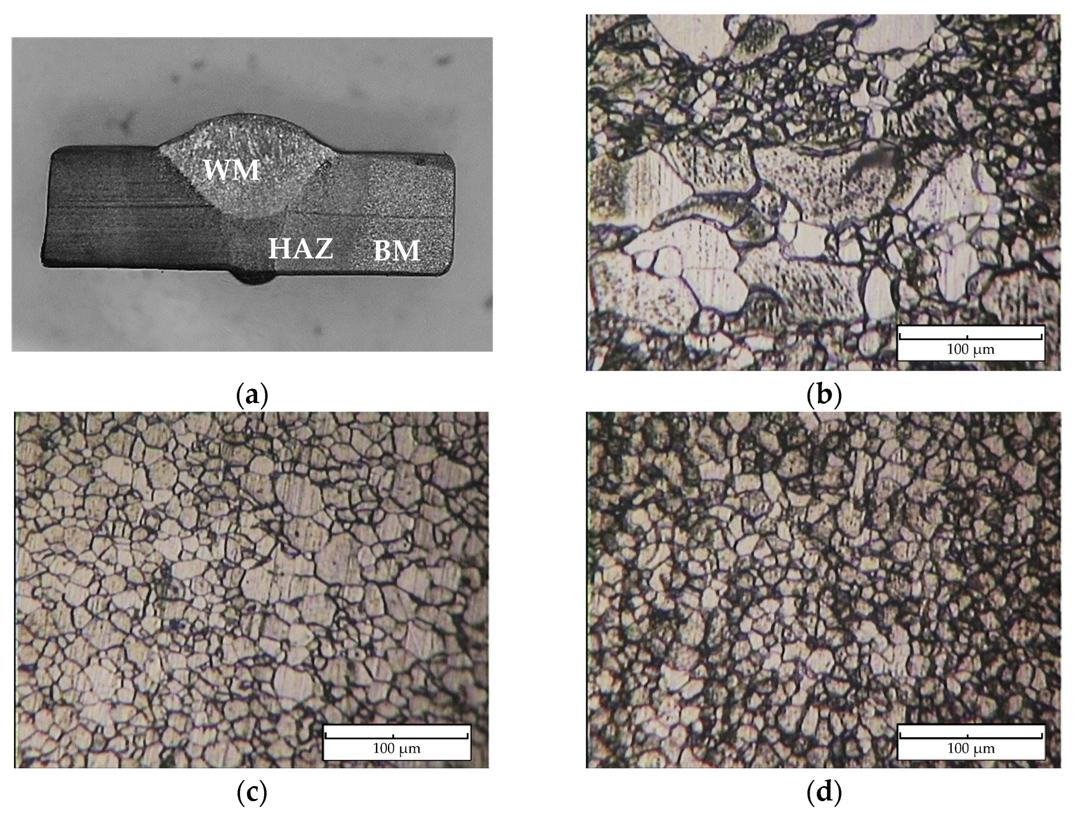
Figure 5 reveals the macro- and microstructure of the specimen’s welded joint. There are three zones of interest, namely, the weld metal (WM), heat-affected zone (HAZ), and base metal (BM), as illustrated in Figure 5a. The weld metal microstructure, as shown in Figure 5b, displays a microstructure characterized by grain boundaries of the acicular, polygonal form of ferrite and perlite, with an average grain size of 21.5 μm. The weld metal’s (Figure 5b) varied microstructure, with large and small grains, stems from the complex thermal cycles in Shielded Metal Arc Welding (SMAW). Rapid heating and cooling due to the welding arc’s high heat cause differing cooling rates across the weld. Slower cooling fosters larger grains in the center, while faster cooling near the edges forms smaller grains. This heterogeneous microstructure results from the SMAW’s localized high-heat input, influenced by the welding parameters and base metal composition. Furthermore, a microstructural inspection of the heat-affected zone, as shown in Figure 5c, is a mostly acicular ferrite structure and has small amounts of perlite with a grain size of 12.8 μm. The base metal zone contains ferrite and perlite phases with an approximation size of the grain of 10.3 μm as shown in Figure 5d. The WM zone acquires the lowest average hardness at 167.1 VHN and then is followed by the HAZ at 173.1 VHN and the BM zone at 192.0 VHN. A Vickers hardness profile of the specimen is presented in Figure 6.

Figure 5.
(a) Macrostructure of welded specimen, and microstructure of (b) weld metal (WM), (c) heat-affected zone (HAZ), and (d) base metal (BM).

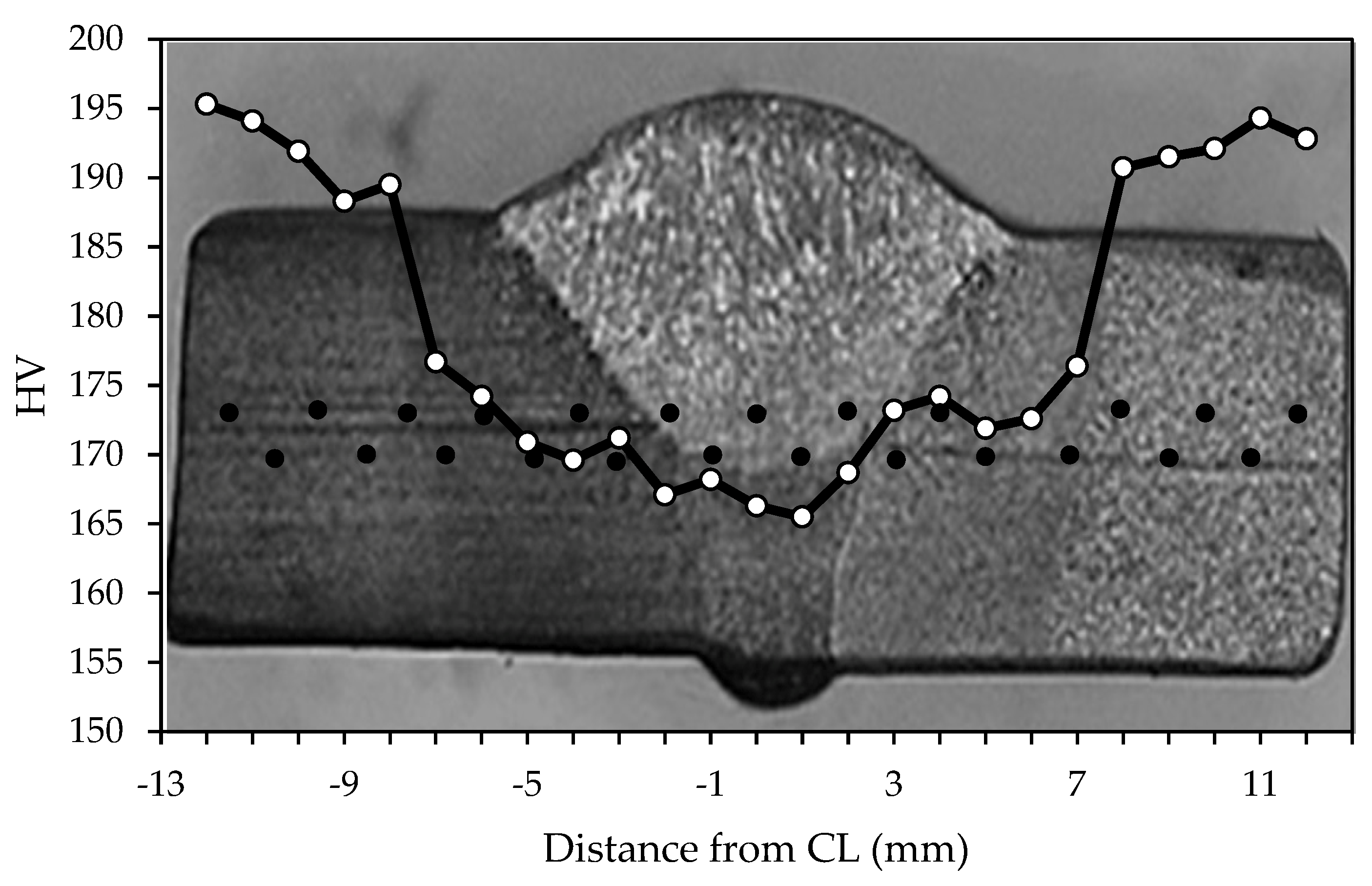
Figure 6.
Hardness profile of the specimen weldment. CL means center line of the weld, and black dot is data collection position.
3.2. Potentiodynamic Polarization
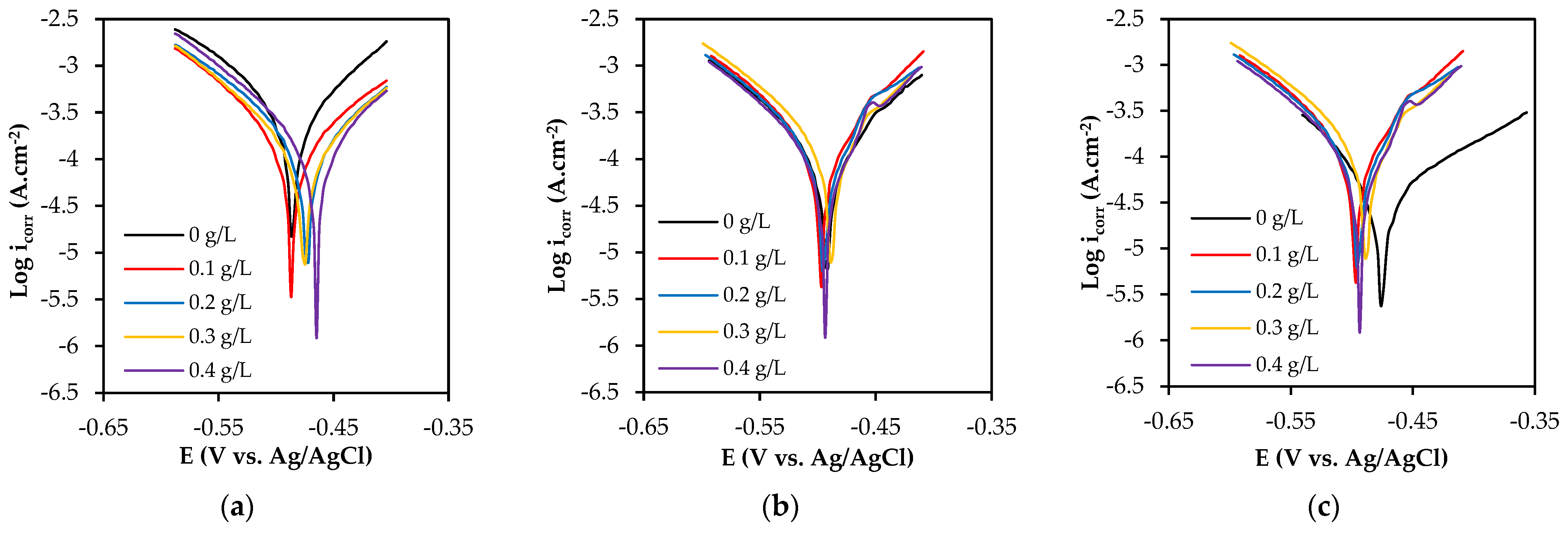
Figure 7 shows the potentiodynamic polarization curves of the specimens tested with different concentrations of SM. The vertical axis represents icorr (current density), which is a measure of the rate of corrosion of a metal or alloy in an electrolyte and expressed in units of amps per square meter (A/cm2). The horizontal axis represents the potential of the electrode in an electrolyte when the potential is varied at a selected rate by applying an electrical source and measured in volts (V) or millivolts (mV) relative to a reference electrode. The curve shift is not easily visible for the three zones as they overlap with each other. The corrosion parameters calculated based on Tafel extrapolation are given in Table 3. SM exhibited an inhibitory effect on the WM zone, as the current density decreased with an increasing concentration. At a concentration of 0.4 g/L, the WM zone showed the lowest corrosion rate of 7.21 mm/year with an inhibition efficiency of 59%. However, at the same concentration, the HAZ indicated an efficiency of 4.28%, with a corrosion rate of 6.84 mm/year. The BM zone had the highest inhibition efficiency of 37% at an extract concentration of 0.2 g/L, resulting in a corrosion rate of 2.74 mm/year.
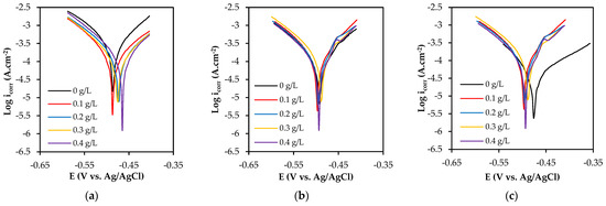
Figure 7.
Typical potentiodynamic polarization (PP) curves of (a) WM, (b) HAZ, and (c) BM for different concentrations of sodium molybdate.
Table 3.
Corrosion parameters calculated from PP curves.
3.3. Observation of Bubbles Detection and H2 Evolution
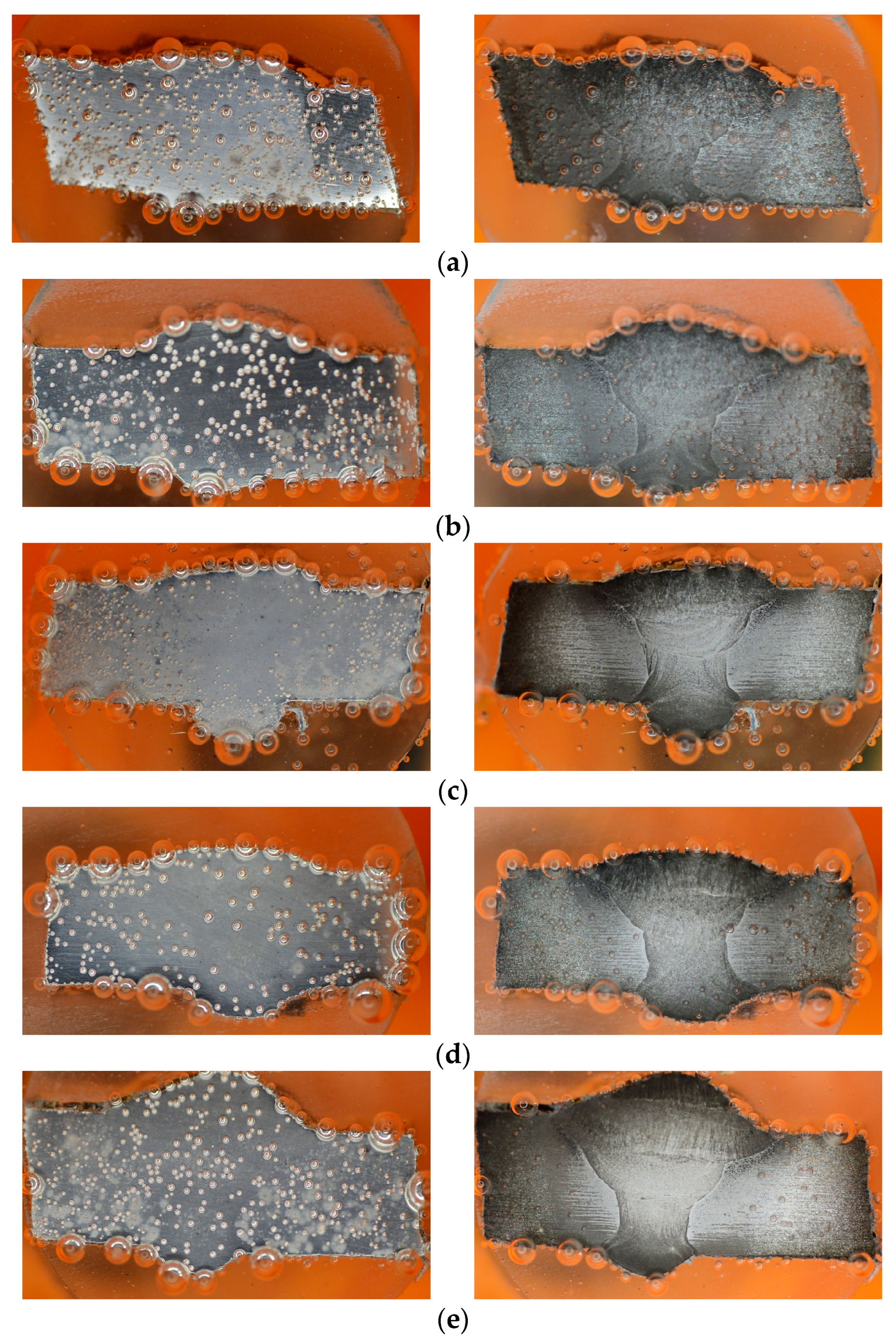
Throughout the duration of the PP test, there was an evolution in the characteristics of the H2 bubbles, based on the images taken at 6 and 10 min (Figure 8). In the blank solution, larger bubbles were observed, initially adhering to the surface before eventually bursting out. Bubbles continued to form intermittently on the specimen’s surface, indicating a partial cathodic reaction taking place to reduce the H⁺ from the H⁺-rich solution (1 M HCl) [38,58]. Conversely, the specimens placed in the inhibitor solution displayed smaller bubbles that diffused across the surface.
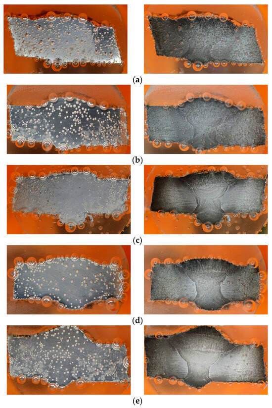
Figure 8.
Images captured during PP test, at 6th minute (left) and 10th minute (right): (a) 0 g/L, (b) 0.1 g/L, (c) 0.2 g/L, (d) 0.3 g/L, and (e) 0.4 g/L.
The training process of YOLOv4 in this study consists of several steps as below:
- Dataset Preparation: Gather 3755 images of the bubble dataset with annotated images and the corresponding bounding boxes around the objects of interest, along with the class labels.
- Configuration: Adjust the hyperparameters in the configuration files. Modify the settings, such as the batch size, learning rate, and input image size (Table 2).
- Training Execution: Execute the training process using the prepared dataset. The model learns to detect objects by minimizing detection errors through optimization.
- Loss Calculation: Compute the loss functions (localization, confidence, and classification) based on the differences between the predicted and true bounding boxes, objectness scores, and class predictions.
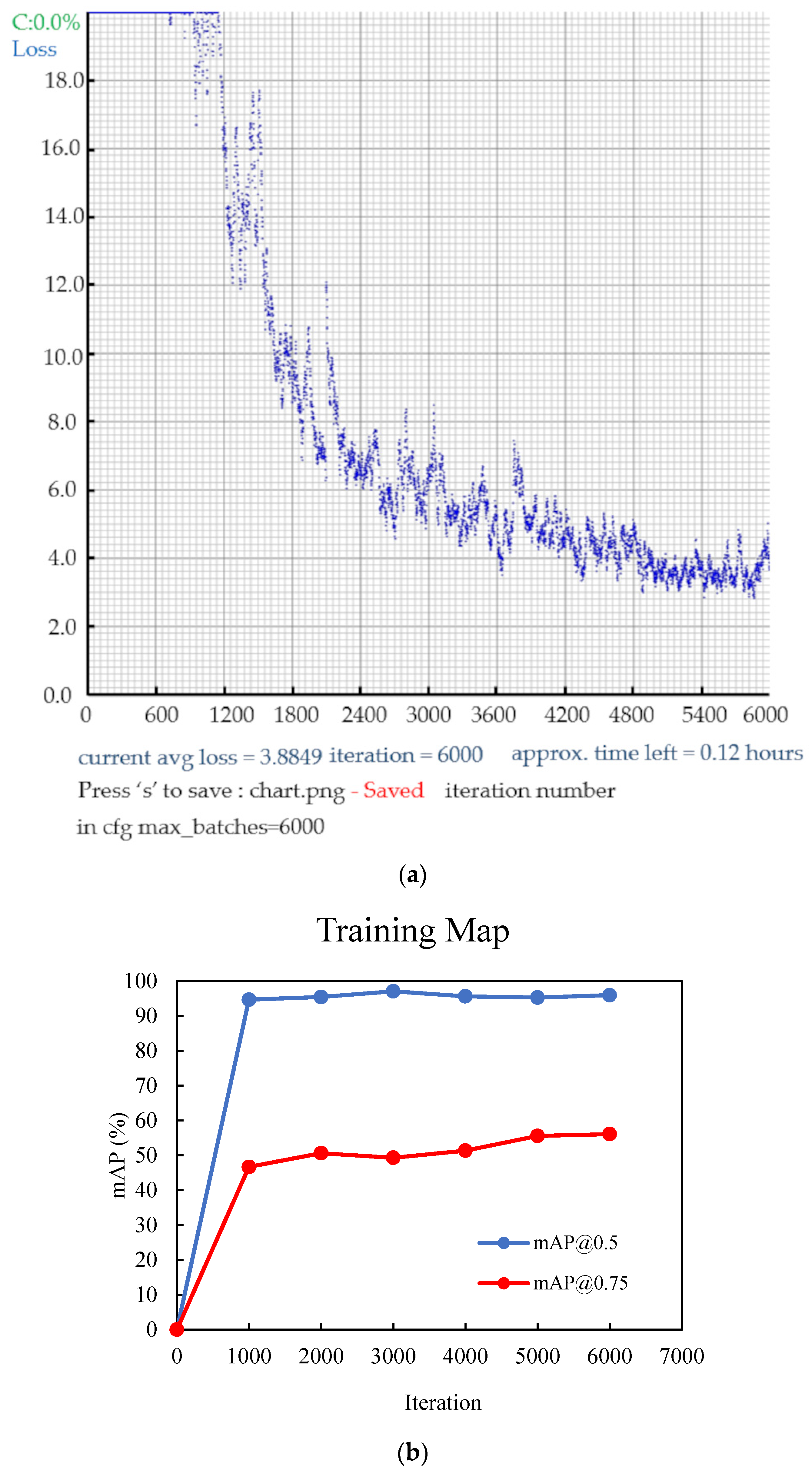
- Backpropagation and Optimization: Backpropagate the calculated loss to optimize the model’s parameters using optimization techniques, like stochastic gradient descent (SGD) or its variants (Figure 9a).
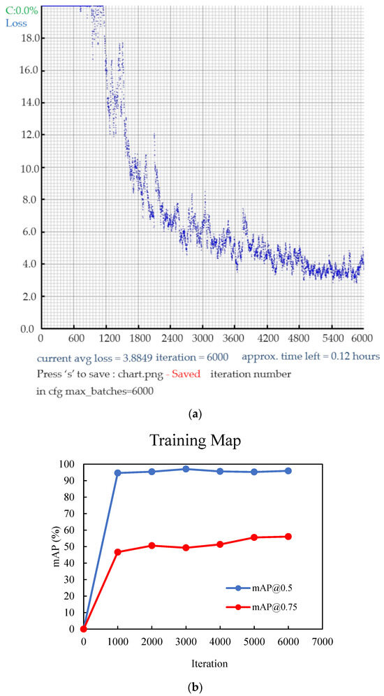 Figure 9. (a) Illustration of the loss progression, and (b) curves of the mAP (mean average precision) during the training of YOLOv4 with the dataset.
 - Model Evaluation: Periodically assess the model’s performance on a validation dataset using metrics, such as precision, recall, and mAP (mean average precision) (Figure 9b).
- Fine-tuning and Iteration: Fine-tune the model by adjusting the hyperparameters or training it on additional data if needed and iterating until the desired accuracy is achieved.
- Model Deployment: Deploy the trained model for inference on new data or integrate it into applications for real-time object detection tasks (Figure 10).
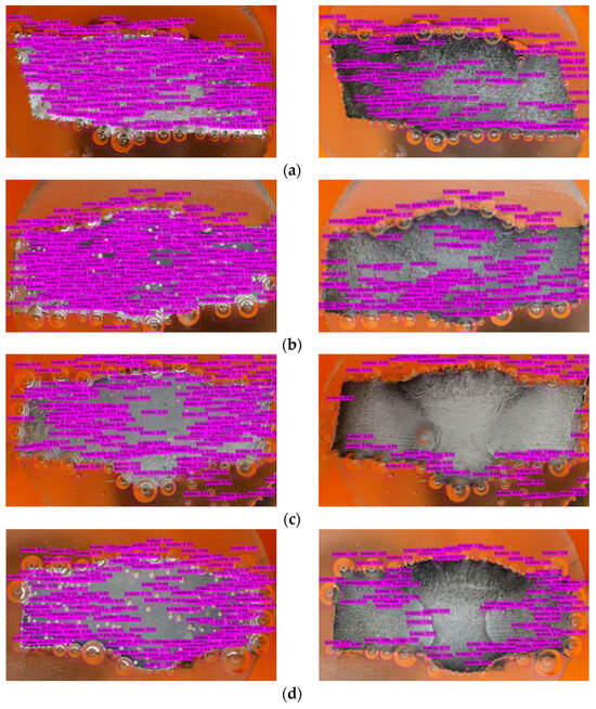
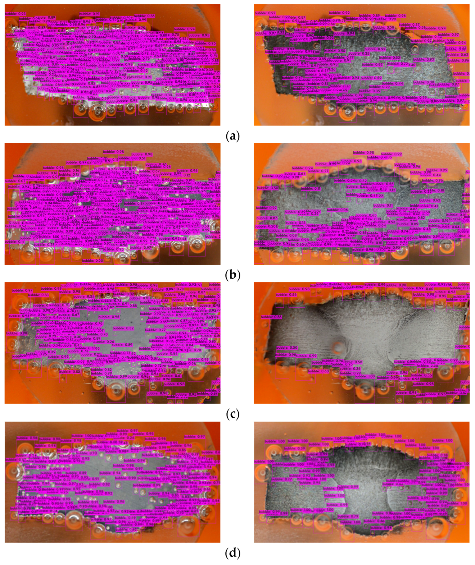
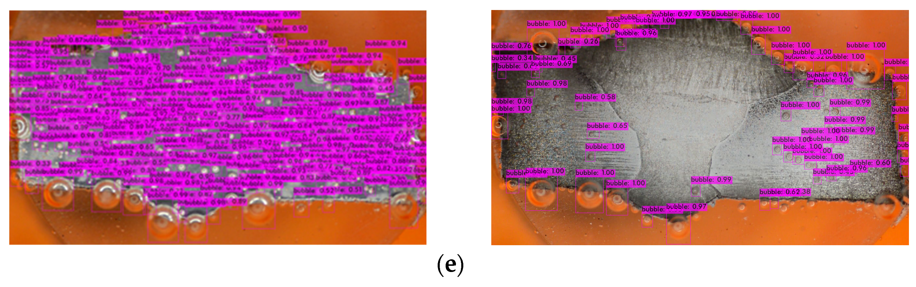
 Figure 10. Bubbles detection in different inhibitory conditions: (a) 0 g/L, (b) 0.1 g/L, (c) 0.2 g/L, (d) 0.3 g/L, and (e) 0.4 g/L.
In order to gain deeper insights from the outcomes, we analyze several calculation results of the detection models trained with the dataset. These results include the mAP50, mAP75, FPS, average IoU, precision, recall, and F1-Score. Precision serves as a metric to assess the accuracy of the model’s predictions by determining the proportion of actual truths correctly identified by the model. Recall measures the ratio of actual truths correctly identified by the model out of the total number of actual truths. The F1-Score is a comprehensive metric that evaluates the balance of the model’s data. It combines precision and recall by calculating their product and dividing it by their sum, multiplied by 2. The IoU, on the other hand, is an indicator that quantifies the extent of the overlap between the bounding box predicted by the object detection model and the actual object. This value is obtained by dividing the overlapped region of the two bounding boxes by the total area covered by the bounding boxes in the image.
In the context of mAP, the term “mAP” stands for mean average precision. AP represents the area under the precision–recall graph. Specifically, mAP is the average value obtained by summing the AP values for each class and dividing it by the total number of classes. A value is usually appended after the mAP to signify the threshold used to determine the reliability of the bounding box when calculating the mAP. The values were recorded at regular intervals, typically every 1000 iterations, during the training process. As depicted in Figure 9a,b, the training has been conducted effectively by reaching a point where the loss has significantly reduced, the accuracy has plateaued, and further improvements are minimal.
Table 4 presents a detailed overview of the test results based on the mAP of the dataset.
Table 4.
Detailed testing results.
The mAP in YOLOv4 serves as an indicator of the bounding box accuracy, which can vary when the model is exposed to new environments or scenarios involving bubbles. However, due to the supervised learning approach employed, the model may struggle to recognize unfamiliar objects [59]. Figure 10 shows that there are a few bubbles that the model fails to identify, and there is a noticeable distinction between the right and left sides of the metal surface. The darker appearance on the right side indicates greater corrosion (after the corrosion process) compared to the relatively less-corroded left side.
The number of bubbles detected in the PP test is given in Table 5. The SM exhibited distinct effects in the WM, HAZ, and BM zones. Subsequently, this count was further divided according to the specific welding areas, namely, the WM, HAZ, and BM. By dividing the number of bubbles detected by the respective area of each welding zone, the ratio between the bubble count and the area for each specific welding area at a given time is obtained.
Table 5.
The number of bubbles detected per unit area (mm2).
The measured volume of the H2 gas (Figure 2b) that evolved during the PP test (from 0 to 10 min) is given in Table 6. The SM demonstrated a different effect on the weld metal (WM) zone and heat-affected zone (HAZ)–base metal (BM) zone.
Table 6.
The measured volume of hydrogen gas that evolved during PP test (×10−4 mL/mm2.s).
Figure 11 shows the comparison between the hydrogen rate and corrosion rate of the specimens tested with different concentrations of SM. The graph shows a similar trend for the H2 evolution rate and corrosion rate.
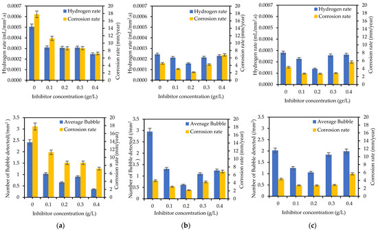
Figure 11.
Hydrogen evolution rate and number of bubbles detected compared with corrosion rate of (a) WM, (b) HAZ, and (c) BM for different concentrations of sodium molybdate.
3.4. SEM and FTIR Observation
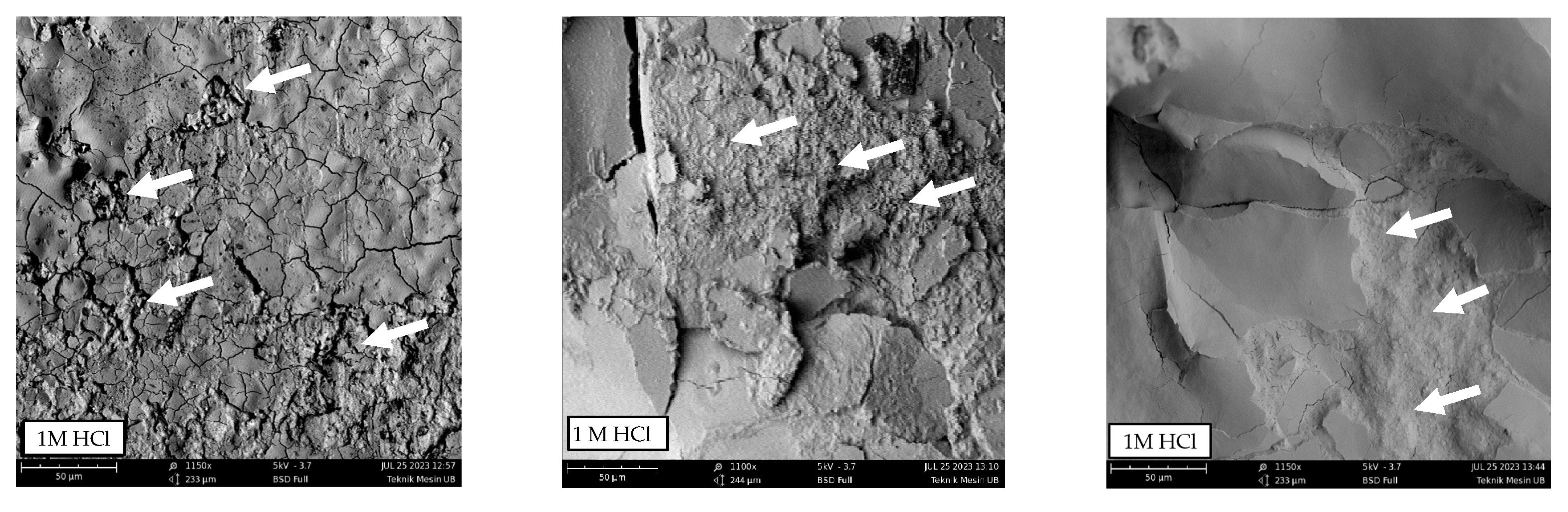
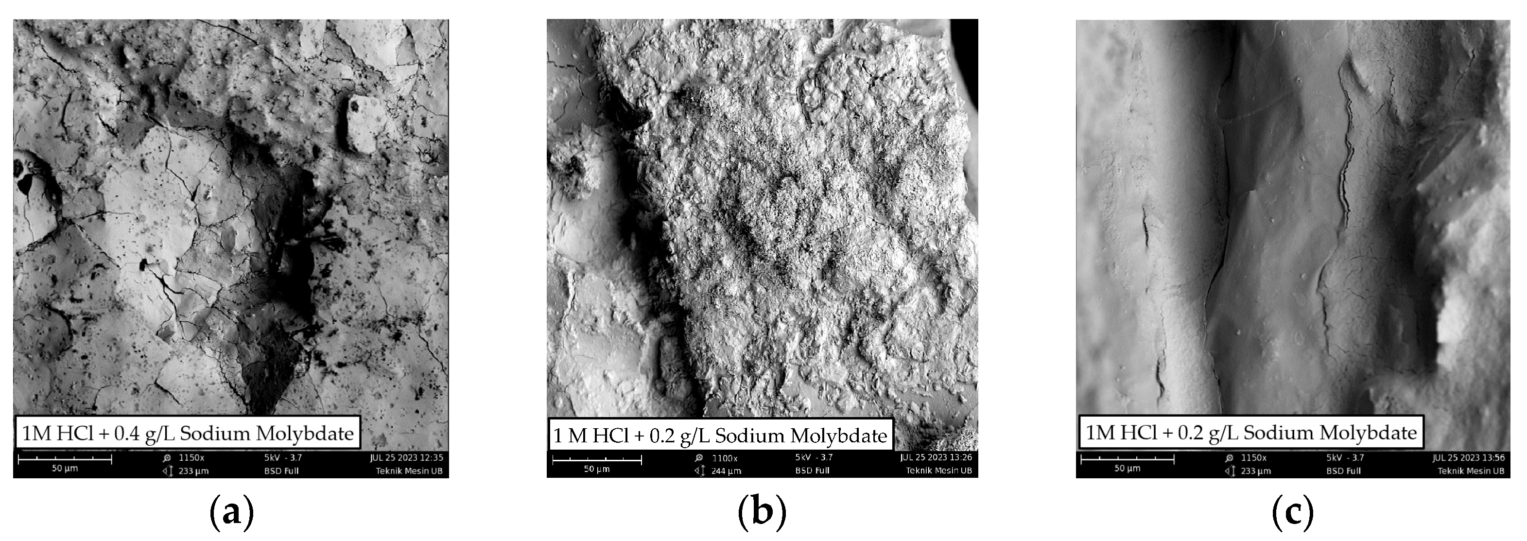
Based on Table 3, the maximum inhibition efficiency of the SM solution for each zone is WM 0.4 g/L, HAZ 0.2 g/L, and BM 0.2 g/L. An immersion test was carried out between the specimens with the SM solution and without the SM solution, which aims to obtain an overview of the surface morphology of each specimen. The surface morphology of the specimens after 5 days of immersion are shown in Figure 12. On the metal surface, several cracks and deposits occurred after being immersed in HCl and HCl + SM. However, the layer of sediment formed in HCl + SM is more even than when immersed in HCl (arrows indicate the areas with minimal sediment). This observation shows how the inhibitory effect of the SM solution restrains the corrosion process.

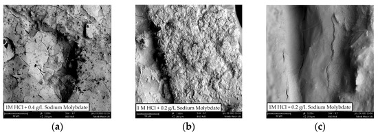
Figure 12.
SEM photograph of metal weldment after being immersed for 5 days in 1 M HCl and 1 M HCl + Sodium Molybdate: (a) WM, (b) HAZ, and (c) BM.
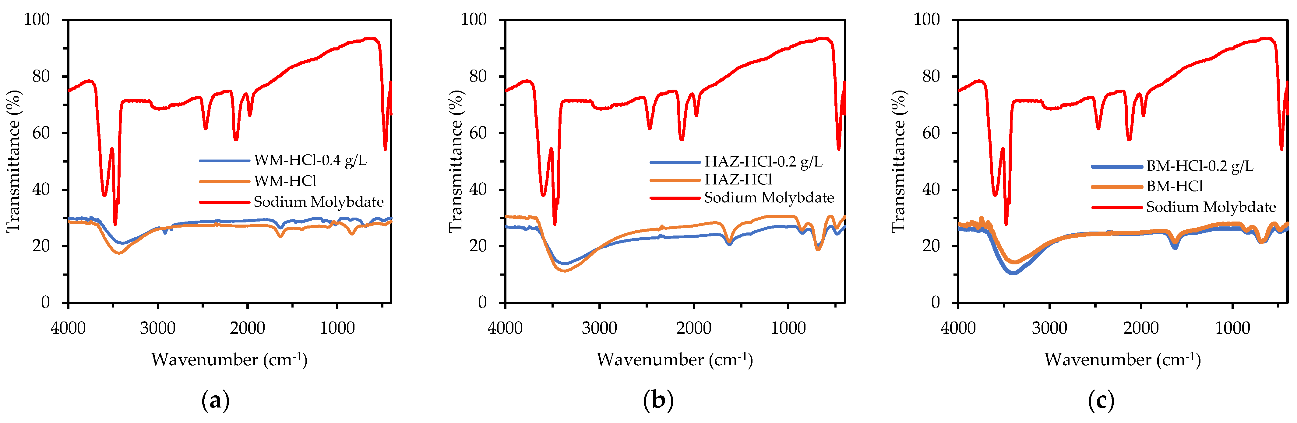
Figure 13 depicts the FTIR spectra of the SM [60] and all the specimens after 5 days of immersion in 1 M HCl and 1 M HCl + SM. Different bonds appeared in the spectra of the weldment specimens when compared to the original SM spectra. There was a peak of about 1630 cm−1 after immersion in HCl, showing a bending vibration of O-H, and weak absorption around 680 cm−1, indicating a link with Fe (hematite). The intensity of these two peaks decreased after immersion in HCl + SM, indicating the development of hematite groups (stable iron oxide, Fe2O3) rather than OH bonds (iron hydroxide).
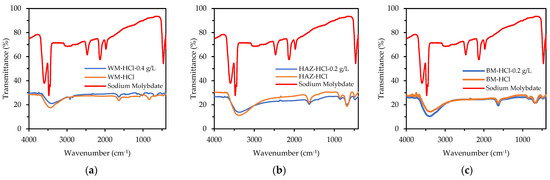
Figure 13.
FTIR spectra of (a) WM, (b) HAZ, and (c) BM zone after being immersed for 5 days in 1 M HCl and 1 M HCl + sodium molybdate (0.4 g/L for WM, and 0.2 g/L for HAZ and BM).
The examination through an EDS analysis demonstrated a rise in the oxygen content as shown in Table 7. This suggests the development of certain oxides that have enveloped the surface of the metal, potentially in the form of Fe(OH)2 [7].
Table 7.
Detection of elements on the specimen surface by using EDS.
The hardness test conducted on the three zones of the weldment indicates that the BM zone exhibits the highest level of hardness. This can be attributed to a microstructure characterized by a smaller grain size, which leads to a bigger volume of grain boundaries [17]. The microstructure of the HAZ consists of acicular ferrite and a fine–coarse grain structure. Meanwhile, the primary microstructure of the WM zone is predominantly determined by the grain boundary of ferrite (as depicted in Figure 5). This is associated with a low cooling rate and the process of ferrite formation facilitated by carbon diffusion. Such a microstructure is less effective in inhibiting corrosion compared to a structure with more grain boundaries. Fewer grain boundaries facilitate the diffusion of Cl− ions. The increased volume of the grain boundaries enhances the chemical activities involved in surface corrosion, thereby promoting the formation of a dense and highly stable passive film that provides superior protection [17]. The WM zone exhibits the highest corrosion in the HCl solution due to its larger grain size and lower hardness. It is well established that metals with a lower hardness possess lower corrosion resistance [61]. Furthermore, the presence of precipitates formed during the welding process contributes to the elevated corrosion rate observed in the WM zone [62]. These precipitates often contain non-metallic elements that have the potential to accelerate the corrosion kinetics [62].
During the duration of the PP test, there were observable changes in the properties of the H2 bubbles (Figure 8 and Figure 11). When analyzing the images taken at the Ecorr, it was noted that fewer bubbles were identified on the samples submerged in a solution containing 0.4 g/L of inhibitor, particularly in the WM area. In contrast, a distinct trend was observed in the HAZ and BM regions, where the lowest bubble counts were detected for the specimens immersed in a solution with 0.2 g/L of inhibitor. This variance could be attributed to variations in the microstructural characteristics of the HAZ and BM regions when compared to the WM zone. The coarser grain structure of the WM area does not facilitate the development of a tightly protective layer, resulting in a more active corrosion environment [17] and encouraging the formation of more bubbles.
In the samples without inhibitors, the bubbles tend to exhibit larger sizes compared to those found in the samples containing inhibitors (Figure 8). Furthermore, an analysis of the bubble detection through a deep learning model reveals that the quantity of bubbles is higher in the absence of inhibitors when contrasted with their presence (refer to Table 5). Persistent bubbles appeared intermittently on the surface of the specimen, indicating a partial cathodic reaction to reduce the presence of H+ ions in the H+-rich solution (1 M HCl) [35,56]. Following the polarization potential surpassing the corrosion potential Ecorr point, there was a gradual reduction in bubble formation, eventually leading to the point where no bubbles were visually observed at the last process of the PP test. This observation aligns with the corrosion process transitioning into the anodic reaction phase. The quantified amount of H2 gas produced during the PP test (as shown in Figure 11a–c) validates the results obtained from the deep learning-based bubble detection. The rate of H2 evolution exhibits a parallel pattern with the corrosion rate, consequently reflecting the trend in inhibitor effectiveness, as indicated in Table 3. A direct correlation can be observed: the fewer H2 bubbles detected, the lower the recorded volume of H2 gas, and the higher the inhibition efficiency (IE). Hence, conducting a quantitative assessment of H2 bubble properties and H2 gas volume should yield a strong correlation with IE.
3.5. Proposed Mechanism of Inhibition
The following description provides the ways through which SM inhibits corrosion. Anodic and cathodic reactions take place in acidic solution conditions (pH < 7) as follows:
The following equation explains how surface iron atoms can react with hydrogen ions forming corrosion:
Fe2+ is unstable and can form a relatively stable FeOOH film after reacting with O2. Moreover, the FeOOH changes into the stable iron oxidation Fe2O3/Fe3O4. Because the generated corrosion layer separates the solution from the steel surface, the corrosion rate gradually decreases as the corrosion production builds up [63].
The negatively charged chloride ions (Cl−) can interact with positively charged iron ions (Fe2+/Fe3+) in the solution. It can aggressively erode the corrosion product layer, enhance the capacity of oxygen species to penetrate, and eventually speed up the corrosion of iron:
When molybdate is added to a 1 M HCl solution, the chloride ions that were previously trapped between the host layers are exchanged for molybdate ions. In a 1 M HCl solution, the components of the passive film [FeMoO4 and Fe2(MoO4)3] are generated after the molybdate ions from the double-layered hydroxides are released into the solution and inhibit the corrosion in steel. The following reactions arise [64]:
The inhibition mechanism of the sodium molybdate solution in HCl to metal weldment relies on the interaction of molybdate ions with the metal surface through adsorption and passivation. Sodium molybdate, acting as a corrosion inhibitor, binds to the iron oxide/molybdate film formed on the metal weldment surface in acidic environments. This film acts as a barrier, hindering aggressive anions like Cl− from reaching the metal surface and preventing metal cations from leaching into the solution [65]. Furthermore, the adsorption of molybdate ions diminishes the corrosion potential and bolsters the corrosion resistance of metal [66]. Schematic of the inhibition mechanism of Sodium Molybdate can be seen in Figure 14. The effectiveness of the sodium molybdate solution in HCl as an inhibitor hinges on multiple factors, including the concentration, inhibitor type and ratio, and prevailing environmental conditions [66,67,68].
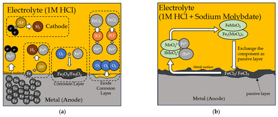
Figure 14.
The corrosion mechanism is shown schematically (a) during the corrosion process in 1 M HCl solution without sodium molybdate and (b) the process when molybdate inhibits the corrosion process of the metal.
4. Conclusions
This study shows how sodium molybdate is used to suppress corrosion, and steel weldments have a different corrosion behavior. This is validated not just through the outcomes of potentiodynamic polarization and hydrogen collection examinations but also via the detection of bubbles employing the YOLOv4 deep learning model.
- With varying efficacy for each weldment zone, sodium molybdate boosts the weldment’s corrosion resistance in 1 M HCl solution. The oxide layer’s stability is increased by the sodium molybdate’s mixed-type inhibition, which also increases the weldment’s corrosion resistance.
- The weld metal’s maximal inhibitory efficiency of the SM solution reached 59% with 0.4 g/L, the heat-affected zone at 52% with 0.2 g/L, and the base metal at 37% with 0.2 g/L of extract.
- The results of training the deep learning model using 3755 bubble images on the mAP50 reached 97.11%, showing that the minimum average bubble detected for the WM was 0.353 /mm2 at an SM concentration of 0.4 g/L, while the HAZ was 0.612 /mm2 at 0.2 g /L, and the BM was 1.055 /mm2 at 0.2 g/L.
- The results from the three conducted tests—potentiodynamic polarization, hydrogen collection examinations, and bubble detection examinations (using deep learning)—display a consistent pattern regarding corrosion behavior. This suggests the potential application of deep learning techniques to analyze corrosion behavior in different scenarios.
This investigation confirms the efficacy of sodium molybdate as a corrosion inhibitor for steel weldments in acidic environments. Achieving optimal corrosion protection involves utilizing different inhibitor doses for distinct weldment zones. Employing machine learning techniques to analyze bubble generation on the weld surface allows for the identification of corrosion behavior.
Author Contributions
Conceptualization, F.A.A.; Methodology, F.A.A. and F.G.; Formal Analysis, F.A.A., C.-C.C. and F.G.; Investigation, F.A.A.; Data Curation, F.A.A. and F.G.; Writing—Original Draft, F.A.A.; Writing—Review and Editing, F.A.A., C.-C.C. and F.G.; Visualization, F.A.A. All authors have read and agreed to the published version of the manuscript.
Funding
This research received no external funding.
Institutional Review Board Statement
Not applicable.
Informed Consent Statement
Not applicable.
Data Availability Statement
The data presented in this study are available on request from the corresponding author. The data are not publicly available due to privacy.
Conflicts of Interest
The authors declare no conflicts of interest.
References
- Nuthalapati, S.; Kee, K.E.; Pedapati, S.R.; Jumbri, K. A Review of Chloride Induced Stress Corrosion Cracking Chracterization in Austenitic Stainless Steels Using Acoustic Emission Technique. Nucl. Eng. Technol. 2023, in press. [CrossRef]
- Usman, B.J.; Umoren, S.A.; Gasem, Z.M. Inhibition of API 5L X60 Steel Corrosion in CO2-Saturated 3.5% NaCl Solution by Tannic Acid and Synergistic Effect of KI Additive. J. Mol. Liq. 2017, 237, 146–156. [Google Scholar] [CrossRef]
- Bahlakeh, G.; Ramezanzadeh, M.; Ramezanzadeh, B. Experimental and Theoretical Studies of the Synergistic Inhibition Effects between the Plant Leaves Extract (PLE) and Zinc Salt (ZS) in Corrosion Control of Carbon Steel in Chloride Solution. J. Mol. Liq. 2017, 248, 854–870. [Google Scholar] [CrossRef]
- Murugadoss, P.; Jeyaseelan, C. Utilization of Silicon from Lemongrass Ash Reinforcement with ADC 12 (Al-Si alloy) Aluminium on Mechanical and Tribological Properties. Silicon 2023, 15, 1413–1428. [Google Scholar] [CrossRef]
- Gapsari, F.; Soenoko, R.; Suprapto, A.; Suprapto, W. Bee Wax Propolis Extract as Eco-Friendly Corrosion Inhibitors for 304SS in Sulfuric Acid. Int. J. Corros. 2015, 2015, e567202. [Google Scholar] [CrossRef]
- Gapsari, F.; Darmadi, D.B.; Setyarini, P.H.; Wijaya, H.; Madurani, K.A.; Juliano, H.; Sulaiman, A.M.; Hidayatullah, S.; Tanji, A.; Hermawan, H. Analysis of Corrosion Inhibition of Kleinhovia Hospita Plant Extract Aided by Quantification of Hydrogen Evolution Using a GLCM/SVM Method. Int. J. Hydrogen Energy 2023, 48, 15392–15405. [Google Scholar] [CrossRef]
- Tristijanto, H.; Ilman, M.N.; Tri Iswanto, P. Corrosion Inhibition of Welded of X—52 Steel Pipelines by Sodium Molybdate in 3.5% NaCl Solution. Egypt. J. Pet. 2020, 29, 155–162. [Google Scholar] [CrossRef]
- Gapsari, F.; Darmadi, D.B.; Setyarini, P.H.; Izzuddin, H.; Madurani, K.A.; Tanji, A.; Hermawan, H. Nephelium lappaceum Extract as an Organic Inhibitor to Control the Corrosion of Carbon Steel Weldment in the Acidic Environment. Sustainibility 2021, 13, 12135. [Google Scholar] [CrossRef]
- Finšgar, M.; Jackson, J. Application of Corrosion Inhibitors for Steels in Acidic Media for the Oil and Gas Industry: A Review. Corros. Sci. 2014, 86, 17–41. [Google Scholar] [CrossRef]
- Zhang, Z.; Bai, Y.; Xu, L.; Han, Y.; Jing, H. CMT+P welding process of UNS S32750 super duplex stainless steel. Trans. Mater. Heat Treat. 2022, 43, 197–206. [Google Scholar] [CrossRef]
- Huang, Y.; Huang, J.; Zhang, J.; Yu, X.; Li, Q.; Wang, Z.; Fan, D. Microstructure and Corrosion Characterization of Weld Metal in Stainless Steel and Low Carbon Steel Joint under Different Heat Input. Mater. Today Commun. 2021, 29, 102948. [Google Scholar] [CrossRef]
- Wang, L.W.; Liu, Z.Y.; Cui, Z.Y.; Du, C.W.; Wang, X.H.; Li, X.G. In Situ Corrosion Characterization of Simulated Weld Heat Affected Zone on API X80 Pipeline Steel. Corros. Sci. 2014, 85, 401–410. [Google Scholar] [CrossRef]
- Miranda-Perez, A.F.; Rodriguez-Vargas, B.R.; Calliari, I.; Pezzato, L. Corrosion Resistance of GMAW Duplex Stainless Steels Welds. Materials 2023, 16, 1847. [Google Scholar] [CrossRef] [PubMed]
- Hou, Y.; Nakamori, Y.; Kadoi, K.; Inoue, H.; Baba, H. Initiation Mechanism of Pitting Corrosion in Weld Heat Affected Zone of Duplex Stainless Steel. Corros. Sci. 2022, 201, 110278. [Google Scholar] [CrossRef]
- Ma, Q.; Luo, C.; Liu, S.; Li, H.; Wang, P.; Liu, D.; Lei, Y. Investigation of Arc Stability, Microstructure Evolution and Corrosion Resistance in Underwater Wet FCAW of Duplex Stainless Steel. J. Mater. Res. Technol. 2021, 15, 5482–5495. [Google Scholar] [CrossRef]
- Zhang, Z.; Han, Y.; Lu, X.; Zhang, T.; Bai, Y.; Ma, Q. Effects of N2 Content in Shielding Gas on Microstructure and Toughness of Cold Metal Transfer and Pulse Hybrid Welded Joint for Duplex Stainless Steel. Mater. Sci. Eng. A 2023, 872, 144936. [Google Scholar] [CrossRef]
- Gollapudi, S. Grain Size Distribution Effects on the Corrosion Behavior of Materials. Corros. Sci. 2012, 62, 90–94. [Google Scholar] [CrossRef]
- Khalaj, G.; Khalaj, M. Investigating the corrosion of the Heat-Affected Zones (HAZs) of API-X70 pipeline steels in aerated carbonate solution by electrochemical methods. Int. J. Press. Vessel. Pip. 2016, 145, 1–12. [Google Scholar] [CrossRef]
- Moat, R.J.; Ooi, S.; Shirzadi, A.A.; Dai, H.; Mark, A.F.; Bhadeshia, H.K.D.H.; Withers, P.J. Residual stress control of multipass welds using low transformation temperature fillers. Mater. Sci. Technol. 2018, 34, 519–528. [Google Scholar] [CrossRef]
- Gach, S.; Schwedt, A.; Olschok, S.; Reisgen, U.; Mayer, J. Confirmation of tensile residual stress reduction in electron beam welding using low transformation temperature materials (LTT) as localized metallurgical injection e Part 1: Metallographic analysis. Mater. Test. 2017, 59, 148–154. [Google Scholar] [CrossRef]
- Chen, X.; Fang, Y.; Li, P.; Yu, Z.; Wu, X.; Li, D. Microstructure, residual stress and mechanical properties of a high strength steel weld using low transformation temperature welding wires. Mater. Des. 2015, 65, 1214–1221. [Google Scholar] [CrossRef]
- Gach, S.; Olschok, S.; Francis, J.A.; Reisgen, U. Confirmation of tensile residual stress reduction in electron beam welding using low transformation temperature materials (LTT) as localized metallurgical injections e Part 2: Residual stress measurement. Mater. Test. 2017, 59, 618–624. [Google Scholar] [CrossRef]
- Fang, J.X.; Li, S.B.; Dong, S.Y.; Wang, Y.J.; Huang, H.S.; Jiang, Y.L.; Liu, B. Effects of phase transition temperature and preheating on residual stress in multi-phase & multi-layer laser metal deposition. J. Alloys Compd. 2019, 792, 928–937. [Google Scholar] [CrossRef]
- Lee, C.H.; Chang, K.H. Prediction of residual stresses in high strength carbon steel pipe weld considering solid-state phase transformation effects. Comput. Struct. 2011, 89, 256–265. [Google Scholar] [CrossRef]
- Wang, X.; Hu, L.; Xu, Q.; Chen, D.; Sun, S. Influence of martensitic transformation on welding residual stress in plates and pipes. Sci. Technol. Weld. Join. 2017, 22, 505–511. [Google Scholar] [CrossRef]
- Ramjaun, T.I.; Stone, H.J.; Karlsson, L.; Gharghouri, M.A.; Dalaei, K.; Moat, R.J.; Bhadeshia, H.K.D.H. Surface residual stresses in multipass welds produced using low transformation temperature filler alloys. Sci. Technol. Weld. Join. 2014, 19, 623–630. [Google Scholar] [CrossRef]
- Fu, Z.H.; Yang, B.J.; Shan, M.L.; Li, T.; Zhu, Z.Y.; Ma, C.P.; Zhang, X.; Gou, G.Q.; Wang, Z.R.; Gao, W. Hydrogen embrittlement behavior of SUS301L-MT stainless steel laser-arc hybrid welded joint localized zones. Corros. Sci. 2020, 164, 108337. [Google Scholar] [CrossRef]
- Ren, X.C.; Zhou, Q.J.; Shan, G.B.; Chu, W.Y.; Li, J.X.; Su, Y.J.; Qiao, L.J. A Nucleation Mechanism of Hydrogen Blister in Metals and Alloys. Met. Mater. Trans. A 2008, 39, 87–97. [Google Scholar] [CrossRef]
- Shan, G.B.; Wang, Y.W.; Chu, W.Y.; Li, J.X.; Hui, X.D. Hydrogen damage and delayed fracture in bulk metallic glass. Corros. Sci. 2005, 47, 2731–2739. [Google Scholar] [CrossRef]
- Song, J.; Curtin, W. Atomic mechanism and prediction of hydrogen embrittlement in iron. Nature Mater. 2013, 12, 145–151. [Google Scholar] [CrossRef]
- Xing, X.; Yu, M.; Chen, W.; Zhang, H. Atomistic simulation of hydrogen-assisted ductile-to-brittle transition in α-iron. Comput. Mater. Sci. 2017, 127, 211–221. [Google Scholar] [CrossRef]
- Lu, B.T.; Luo, J.L.; Norton, P.R.; Ma, H.Y. Effects of dissolved hydrogen and elastic and plastic deformation on active dissolution of pipeline steel in anaerobic groundwater of near-neutral pH. Acta Mater 2009, 57, 41–49. [Google Scholar] [CrossRef]
- Li, M.C.; Cheng, Y.F. Mechanistic investigation of hydrogen-enhanced anodic dissolution of X-70 pipe steel and its implication on near-neutral pH SCC of pipelines. Electrochim. Acta 2007, 52, 8111–8117. [Google Scholar] [CrossRef]
- Atta, N.F.; Fekry, A.M.; Hassaneen, H.M. Corrosion inhibition, hydrogen evolution and antibacterial properties of newly synthesized organic inhibitors on 316L stainless steel alloy in acid medium. Int. J. Hydrogen Energy 2011, 36, 6462–6471. [Google Scholar] [CrossRef]
- Singh, A.; Ansari, K.R.; Quraishi, M.A.; Kaya, S.; Erkan, S. Chemically Modified Guar Gum and Ethyl Acrylate Composite as a New Corrosion Inhibitor for Reduction in Hydrogen Evolution and Tubular Steel Corrosion Protection in Acidic Environment. Int. J. Hydrogen Energy 2021, 46, 9452–9465. [Google Scholar] [CrossRef]
- Ameer, M.A.; Fekry, A.M. Inhibition effect of newly Synthesized Heterocyclic Organic Molecules on Corrosion of Steel in Alkaline Medium Containing Chloride. Int. J. Hydrogen Energy 2010, 35, 11387–11396. [Google Scholar] [CrossRef]
- King, A.D.; Birbilis, N.; Scully, J.R. Accurate Electrochemical Measurement of Magnesium Corrosion Rates; a Combined Impedance, Mass-Loss and Hydrogen Collection Study. Electrochim. Acta 2014, 121, 394–406. [Google Scholar] [CrossRef]
- Fekry, A.M.; Ameer, M.A. Electrochemical Investigation on the Corrosion and Hydrogen Evolution Rate of Mild Steel in Sulphuric Acid Solution. Int. J. Hydrogen Energy 2011, 36, 11207–11215. [Google Scholar] [CrossRef]
- El-Meligi, A.A.; Ismail, N. Hydrogen Evolution Reaction of Low Carbon Steel Electrode in Hydrochloric Acid as a Source for Hydrogen Production. Int. J. Hydrogen Energy 2009, 34, 91–97. [Google Scholar] [CrossRef]
- Azizi, O.; Jafarian, M.; Gobal, F.; Heli, H.; Mahjani, M.G. The Investigation of the Kinetics and Mechanism of Hydrogen Evolution Reaction on Tin. Int. J. Hydrogen Energy 2007, 32, 1755–1761. [Google Scholar] [CrossRef]
- Zhang, A.; Lipton, Z.C.; Li, M.; Smola, A.J. Dive into Deep Learning; Cambridge University Press: Cambridge, UK, 2023. [Google Scholar]
- Sarker, I.H. Deep Learning: A Comprehensive Overview on Techniques, Taxonomy, Applications and Research Directions. Sn. Comput. Sci. 2021, 2, 420. [Google Scholar] [CrossRef]
- Redmon, J.; Divvala, S.; Girshick, R.; Farhadi, A. You Only Look Once: Unified, Real-Time Object Detection. In Proceedings of the 2016 IEEE Conference on Computer Vision and Pattern Recognition (CVPR), Las Vegas, NV, USA, 27–30 June 2016; pp. 779–788. [Google Scholar] [CrossRef]
- Wang, C.Y.; Bochkovskiy, A.; Liao, H.Y.M. Scaled YOLOv4: Scaling Cross Stage Partial Network. In Proceedings of the IEEE/CVF Conference on Computer Vision and Pattern Recognition (CVPR), New Orleans, LA, USA, 19–20 June 2021; pp. 13029–13038. [Google Scholar]
- Bochkovskiy, A.; Wang, C.-Y.; Liao, H.Y.M. YOLOv4: Optimal Speed and Accuracy of Object Detection. arXiv 2020, arXiv:2004.10934. [Google Scholar] [CrossRef]
- Ser, C.T.; Žuvela, P.; Wong, M.W. Prediction of Corrosion Inhibition Efficiency of Pyridines and Quinolines on an Iron Surface Using Machine Learning-Powered Quantitative Structure-Property Relationships. Appl. Surf. Sci. 2020, 512, 145612. [Google Scholar] [CrossRef]
- Varvara, S.; Berghian-Grosan, C.; Bostan, R.; Ciceo, R.L.; Salarvand, Z.; Talebian, M.; Raeissi, K.; Izquierdo, J.; Souto, R.M. Experimental Characterization, Machine Learning Analysis and Computational Modelling of the High Effective Inhibition of Copper Corrosion by 5-(4-pyridyl)-1,3,4-oxadiazole-2-thiol in Saline Environment. Electrochim. Acta 2021, 398, 139282. [Google Scholar] [CrossRef]
- Aghaaminiha, M.; Mehrani, R.; Colahan, M.; Brown, B.; Singer, M.; Nesic, S.; Vargas, S.M.; Sharma, S. Machine Learning Modeling of Time-Dependent Corrosion Rates of Carbon Steel in Presence of Corrosion Inhibitors. Corros. Sci. 2021, 193, 109904. [Google Scholar] [CrossRef]
- AWS A5.1/A5.1M:2012; Specification for Carbon Steel Electrodes for Shielded Metal Arc Welding. American Welding Society: Doral, FL, USA, 2012.
- Yun, S.; Han, D.; Chun, S.; Oh, S.J.; Yoo, Y.; Choe, J. CutMix: Regularization Strategy to Train Strong Classifiers with Localizable Features. In Proceedings of the 2019 IEEE/CVF International Conference on Computer Vision (ICCV), Seoul, Republic of Korea, 27 October 2019; pp. 6022–6031. [Google Scholar]
- Ghiasi, G.; Lin, T.-Y.; Le, Q.V. DropBlock: A Regularization Method for Convolutional Networks. In Proceedings of the 32nd International Conference on Neural Information Processing Systems, Red Hook, NY, USA, 3 December 2018; Curran Associates Inc.: New York, NY, USA, 2018; pp. 10750–10760. [Google Scholar]
- Misra, D. Mish: A Self Regularized Non-Monotonic Activation Function. arXiv 2020, arXiv:1908.08681. [Google Scholar] [CrossRef]
- He, K.; Zhang, X.; Ren, S.; Sun, J. Spatial Pyramid Pooling in Deep Convolutional Networks for Visual Recognition. IEEE Trans. Pattern Anal. Mach. Intell. 2015, 37, 1904–1916. [Google Scholar] [CrossRef] [PubMed]
- Woo, S.; Park, J.; Lee, J.-Y.; Kweon, I.S. CBAM: Convolutional Block Attention Module. In Proceedings of the Computer Vision—ECCV 2018; Ferrari, V., Hebert, M., Sminchisescu, C., Weiss, Y., Eds.; Springer: Cham, Switzerland, 2018; pp. 3–19. [Google Scholar]
- Liu, S.; Lu, Q.; Haifang, Q.; Jianping, S.; Jiaya, J. Path Aggregation Network for Instance Segmentation. In Proceedings of the IEEE/CVF Conference on Computer Vision and Pattern Recognition, Salt Lake City, UT, USA, 18 June 2018. [Google Scholar] [CrossRef]
- Zheng, Z.; Ping, W.; Wei, L.; Jinze, L.; Rongguang, Y.; Dongwei, R. Distance-IoU Loss: Faster and Better Learning for Bounding Box Regression. In Proceedings of the AAAI Conference on Artificial Intelligence, Honolulu, HI, USA, 27 January–3 February 2019. [Google Scholar] [CrossRef]
- Alexey Yolo_Mark 2023. Available online: https://github.com/AlexeyAB/Yolo_mark (accessed on 7 February 2023).
- Zimmermann, T.; Hort, N.; Zhang, Y.; Müller, W.-D.; Schwitalla, A. The Video Microscopy-Linked Electrochemical Cell: An Innovative Method to Improve Electrochemical Investigations of Biodegradable Metals. Materials 2021, 14, 1601. [Google Scholar] [CrossRef]
- Ji, S.J.; Ling, Q.H.; Han, F. An improved algorithm for small object detection based on YOLO v4 and multi-scale contextual information. Comput. Electr. Eng. 2023, 105, 8490. [Google Scholar] [CrossRef]
- NIST Chemistry WebBook, SRD 69. Available online: https://webbook.nist.gov/cgi/inchi?ID=B6000473&Mask=80 (accessed on 3 July 2023).
- Zendejas Medina, L.; Tavares da Costa, M.V.; Paschalidou, E.M.; Lindwall, G.; Riekehr, L.; Korvela, M.; Fritze, S.; Kolozsvári, S.; Gamstedt, E.K.; Nyholm, L.; et al. Enhancing Corrosion Resistance, Hardness, and Crack Resistance in Magnetron Sputtered High Entropy CoCrFeMnNi Coatings by Adding Carbon. Mater. Des. 2021, 205, 109711. [Google Scholar] [CrossRef]
- Ashari, R.; Eslami, A.; Shamanian, M.; Asghari, S. Effect of Weld Heat Input on Corrosion of Dissimilar Welded Pipeline Steels under Simulated Coating Disbondment Protected by Cathodic Protection. J. Mater. Res. Technol. 2020, 9, 2136–2145. [Google Scholar] [CrossRef]
- Ma, Y.; Li, Y.; Wang, F. The Effect of β-FeOOH on the Corrosion Behavior of Low Carbon Steel Exposed in Tropic Marine Environment. Mater. Chem. Phys. 2008, 112, 844–852. [Google Scholar] [CrossRef]
- Yan, H.; Wang, J.; Zhang, Y.; Hu, W. Preparation and Inhibition Properties of Molybdate Intercalated ZnAlCe Layered Double Hydroxide. J. Alloys Compd. 2016, 678, 171–178. [Google Scholar] [CrossRef]
- Zatkalikova, V.; Markovicova, L.; Wrobel-Knysak, A. Electrochemical Characheristic of Austenitic Stainless Steel in Mixed Chloride—Molybdate Solutions. Communications 2017, 19, 74–78. [Google Scholar] [CrossRef]
- Rashid, K.H.; Khadom, A.A. Optimization of Inhibitive Action of Sodium Molybdate (IV) for Corrosion of Carbon Steel in Saline Water Using Response Surface Methodology. Korea J. Chem. Eng. 2019, 36, 1350–1359. [Google Scholar] [CrossRef]
- Xu, Z.; Chen, L.; Han, J.; Zhu, C. Properties of Sodium Molybdate-Based Compound Corrosion Inhibitor for Hot-Dip Galvanized Steel in Marine Environment. Corros. Rev. 2023, 41, 225–235. [Google Scholar] [CrossRef]
- Guo, W.; Zhao, X.; Wang, D.; Li, Y.; Zhou, L.; Li, Z.; Gao, Y. Corrosion Behavior of Mild Steel in Presence of 2-Chloromethylbenzimidazole and Sodium Molybdate in 1M HCl. Russ. J. Electrochem 2020, 57, 970–977. [Google Scholar] [CrossRef]


Disclaimer/Publisher’s Note: The statements, opinions and data contained in all publications are solely those of the individual author(s) and contributor(s) and not of MDPI and/or the editor(s). MDPI and/or the editor(s) disclaim responsibility for any injury to people or property resulting from any ideas, methods, instructions or products referred to in the content. |
© 2023 by the authors. Licensee MDPI, Basel, Switzerland. This article is an open access article distributed under the terms and conditions of the Creative Commons Attribution (CC BY) license (https://creativecommons.org/licenses/by/4.0/).