Article

Features of Changes in the Parameters of Acoustic Signals Characteristic of Various Metalworking Processes and Prospects for Their Use in Monitoring

by
Sergey N. Grigoriev
,
Mikhail P. Kozochkin
,
Artur N. Porvatov
,
Vladimir D. Gurin
and
Yury A. Melnik
*
Department of High-Efficiency Processing Technologies, Moscow State University of Technology “STANKIN”, Vadkovskiy per. 3A, 127055 Moscow, Russia
*
Author to whom correspondence should be addressed.
Appl. Sci. 2024, 14(1), 367; https://doi.org/10.3390/app14010367
Submission received: 23 November 2023 / Revised: 23 December 2023 / Accepted: 27 December 2023 / Published: 30 December 2023

Abstract

:
The need to create monitoring systems to equip the technological machinery of automated production determines the relevance of searching for parameters of acoustic signals that carry information about the course of treatment processes. The study of acoustic signals in various types of material processing allowed the identification of general features of changes in their spectral composition associated with variations in the power density of energy impact on processed material. The results of experimental work on various technological equipment, including blade processing and processing with concentrated energy flows, are presented in this work. It is shown that changes in the quality of processing in the form of increased tool wear, the concentration of erosion products during WEDM (wire electrical discharge machining), focal plane displacement during laser processing, etc., lead to a natural change in the ratio of acoustic signal amplitudes in the low frequency and high frequency ranges. This property can be used in monitoring systems for automatic equipment.

1. Introduction

There is a stable trend in the development of modern industrial production, which consists of the desire to minimize human presence in the area of implementation of production processes. For this purpose, the machinery is equipped with additional sensors and signal analysis systems designed not only to replace human organoleptic capabilities but also to perceive better information signals that are inaccessible to human capabilities. To automate production processes, it is not enough to supplement technological equipment with conveyors, manipulators, robots, and other similar devices that replace the manual labor of the operator. It is necessary to monitor the current state of all units, on the operation of which the reliability of the functioning of the equipment and the quality of the obtained products depend. If the process of such expensive equipment is accompanied by accidents, downtime, and the release of defective products, this will lead to a decrease in the economic effect of the automation of production processes.
Among all the problems that arise when creating automated equipment, monitoring the treatment process remains the most difficult. This is because it is almost impossible to place sensors in the processing area, and indirect monitoring methods are associated with the impacts of various random factors and a decrease in the information content of equipment signals when it is located remotely from the core of the technological process [1,2,3,4]. Many problems of monitoring the condition of the blade tool could be solved with systems for monitoring power parameters. However, for industrial applications, such systems should not degrade the dynamic characteristics of the machine and reduce its versatility. Piezoelectric converters made it possible to create dynamometric systems [5] that provide the necessary equipment rigidity and measurement quality, but their use was limited by laboratory conditions. Of all the attempts to measure the power parameters functionally related to the components of the cutting force, the control of the power consumed by the drives providing the relative movement of the tool and the workpiece has found actual industrial application. However, another problem arose here, which is that the drive power must meet the needs of both roughing and finishing. Under these conditions, small drills, cutters, taps and finishing tools are out of the observation area, since it is difficult to distinguish the power consumption for them from the idle power of a powerful engine. Namely, breakdowns of such a tool are the leading cause of equipment downtime and negative impacts on the processed product [6].
A lot of information about the condition of the tools could be obtained if there was a technique for measuring the temperature of the tool cutting edge. However, during cutting, the tool edge is usually covered with separated chips and coolant, and, therefore, is inaccessible for control using modern pyrometers [7,8]. Although the monitoring of temperature changes in electrical equipment, friction surfaces, and bearing units is widely presented in the scientific literature [9,10,11,12,13,14], the use of this technique for monitoring the cutting process can only be observed in experimental studies.
An assessment of the condition of tools using direct measurements or an analysis of their images is relevant only outside the cutting process [15,16,17], which does not allow the method to be widely used for monitoring the technological process itself in the “online” mode.
The analysis of vibroacoustic signals as a method of non-destructive testing has long won a firm place in the industry. It is widely used to control the quality of manufacturing of individual components and finished products, as well as to monitor their conditions during operation. Many studies are devoted to assessing the state of bearing units and gears based on the analysis of their noise and vibrations [18,19,20,21] and the state of various rotary mechanisms [22,23,24,25,26]. Wireless information transmission systems are increasingly being used to control the vibrations of rotating components [24].
Information on the use of acoustic emission signals (AE) for monitoring various technological processes is presented much more modestly in the literature. It can be assumed that the situation is determined by the more complex nature of the occurrence of AE signals and the difficulties of their analysis. At the same time, it was established that AE signals accompany not only technological processes of blade processing but are also observed during phase transformations accompanied by changes in the crystal lattice of the material [27,28,29,30,31], during crystallization and melting of the substance, and during the formation of particles of a new phase in supersaturated solutions [32,33,34,35]. Directly related to the cutting process are works on studying of AE signals during the plastic deformation of materials, accompanied by the development of defects in their structures [36,37,38].
Monitoring the condition of tools operating with relatively low power consumption is possible by monitoring the vibrations accompanying the cutting process. Vibrations can be controlled using accelerometers and microphones installed at a sufficient distance from the cutting area. Changes in the cutting ability of tools find a broad response when changing many parameters of AE signals accompanying cutting. The main disadvantage of diagnostic signals, including AE signals, is that their parameters can change not only due to changes in the state of the cutting tool but also when other cutting conditions change, which include processing modes. If such dependencies have high gradients, then it becomes necessary to train the diagnostic system, which causes specific difficulties, especially in a single production, or to search for parameters that are less dependent on processing modes [6]. To reduce the dependence of AE parameters on the variety of modes and the impacts of other factors, work was carried out where the condition of the diagnostic object was assessed using AE parameters taken in different frequency ranges [39,40,41,42,43,44]. Works in multiparametric diagnostics of the state of the cutting process using the analysis of AE signals in different frequency ranges also began to appear more often [6,45,46,47,48,49,50].
The danger of using AE signal parameters in different frequency ranges is that such parameters may be closely related. In this case, the use of multiparametric diagnostics will not provide additional information and will not justify the complication of the processing algorithm [6,46]. The purpose of this work is to study the physical causes that differentially affect the parameters of the AE signal in different frequency ranges and the possibilities of using several signal parameters to monitor various metalworking processes.

2. Instruments and Technological Equipment

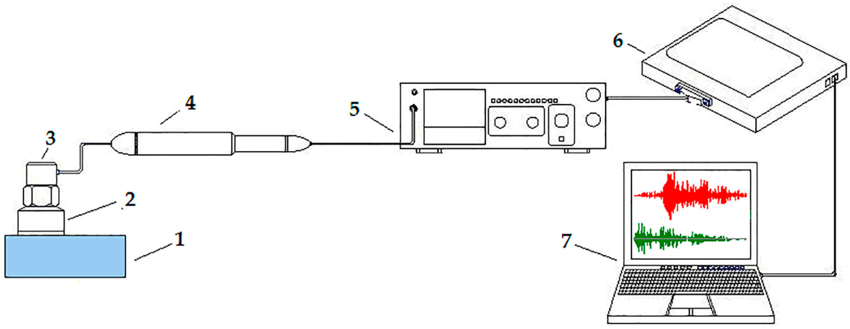
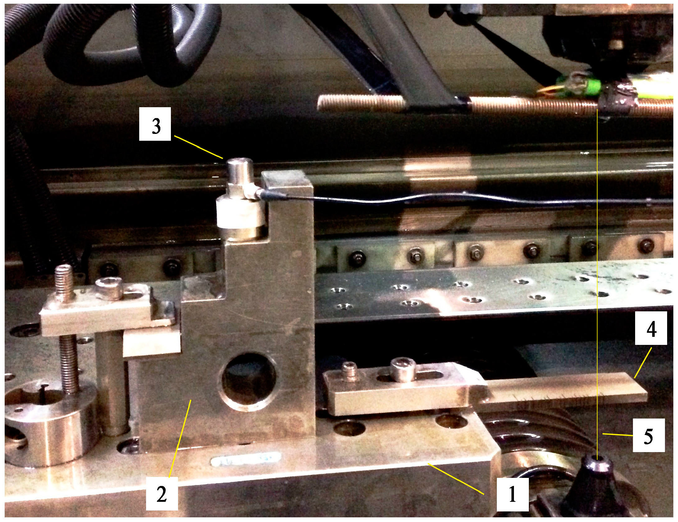
2.1. Instruments for Measuring Vibrations in Metalworking

This article is based on experimental material obtained from studies of AE signals accompanying technological processes on machine tools of various groups. The method of AE registration was almost the same in all experiments. Figure 1 shows a typical scheme for recording AE signals on processing equipment.
The position of the accelerometer was chosen so that there were no movable joints (bearings and guides) between it and the cutting area. The accelerometer was usually attached with a magnet or a threaded connection. Table 1 shows the characteristics of the accelerometers used.
Table 1 indicates the frequency range where the voltage sensitivity of accelerometers has a constant value. However, for comparative assessments of changes in vibroacoustic activity, a more comprehensive range was used, including the resonant frequency and higher. In practice, data were obtained for the frequency range up to 40 kHz.
The digitally saved records (Figure 1) were processed using time and frequency analysis methods. Spectral analysis was used to select the frequency ranges where the amplitudes of AE signals experienced more noticeable changes when the cutting tool condition or process conditions changed. In these ranges, narrow-band frequency filtering and smoothing of recordings were carried out by constructing RMS values of signal amplitudes with different averaging periods. This also helped to reduce the influence of noise on the AE signals, the presence of which is associated with the discreteness of physical processes of materials processing. The results of such processing of AE signals are presented in Section 3.

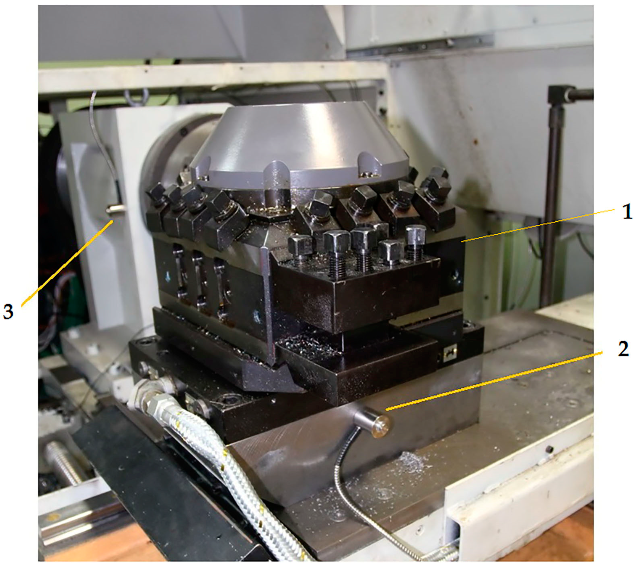
2.2. Technological Equipment under Study

Figure 2 shows an example of a multi-purpose CNC lathe CA700K10F2 (JSC “SASTA”, Russian Federation), where the accelerometers are fixed to the base of the turret and the spindle headstock body using a threaded stud.
Figure 2 depicts two accelerometers, the analysis of the signals of which showed that the signals recorded on the spindle headstock are significantly less informative about the cutting process compared to the accelerometer mounted on the base of the turret. However, the signals received from the surface of the spindle head contain more diagnostic information regarding the condition of the bearings of the front spindle support [26,51]. Figure 3 shows the locations of the vibration sensors on a flat-grinding machine. Since, in this case, the tool was rotating, the sensors were located on the side of the workpiece. The figure shows that in addition to the accelerometer, an acoustic emission sensor and a 3-component dynamometer by Kistler were used in the experiment. Two identical workpieces made of heat-resistant steel Inconel 718 were mounted on the machine using screws.
Figure 4 shows another example of installing an accelerometer on a magnet on the support of a universal lathe for experiments with turning and boring operations on workpieces made of 41CrS4 steel (DIN, EN standards). The accelerometer was located on the support sufficiently far from the processing area.
When conducting studies of AE signals on machines processing with concentrated energy flows, the installation of an accelerometer encountered specific difficulties. The more significant difficulties arose when monitoring AE during electron beam doping in a vacuum chamber. Inserting the accelerometer into the chamber was impossible due to powerful electromagnetic interference and challenges in introducing cables to the sensor through vacuum inlets. To obtain information about the VA signal when applying an electron pulse, it was necessary to use a wire waveguide [50]. Figure 5 shows the vacuum chamber of the “RITM-SP” installation [52] with an open hatch, where the irradiated workpiece with an attached waveguide in the form of a copper wire with a cross-section of 2.1 mm2 is visible. The exact figure shows a scheme for recording AE signals, where a receiving plate (position 3) is installed at the end of the waveguide on which the accelerometer is mounted.
When studying AE signals on WEDM machines, the problem was that the workpiece was immersed in the working fluid during processing. The laboratory equipment was not intended to work in a liquid environment; therefore, the accelerometers were installed on additional stands on the machine worktable. When immersed in the working fluid, the upper part of the stand, along with the accelerometer, remained in the air. Figure 6 shows the installation of the accelerometer in the processing area of the CUT30P WEDM machine (GF Agie Charmilles, Basel, Switzerland).

3. Results of Studies of AE Signals

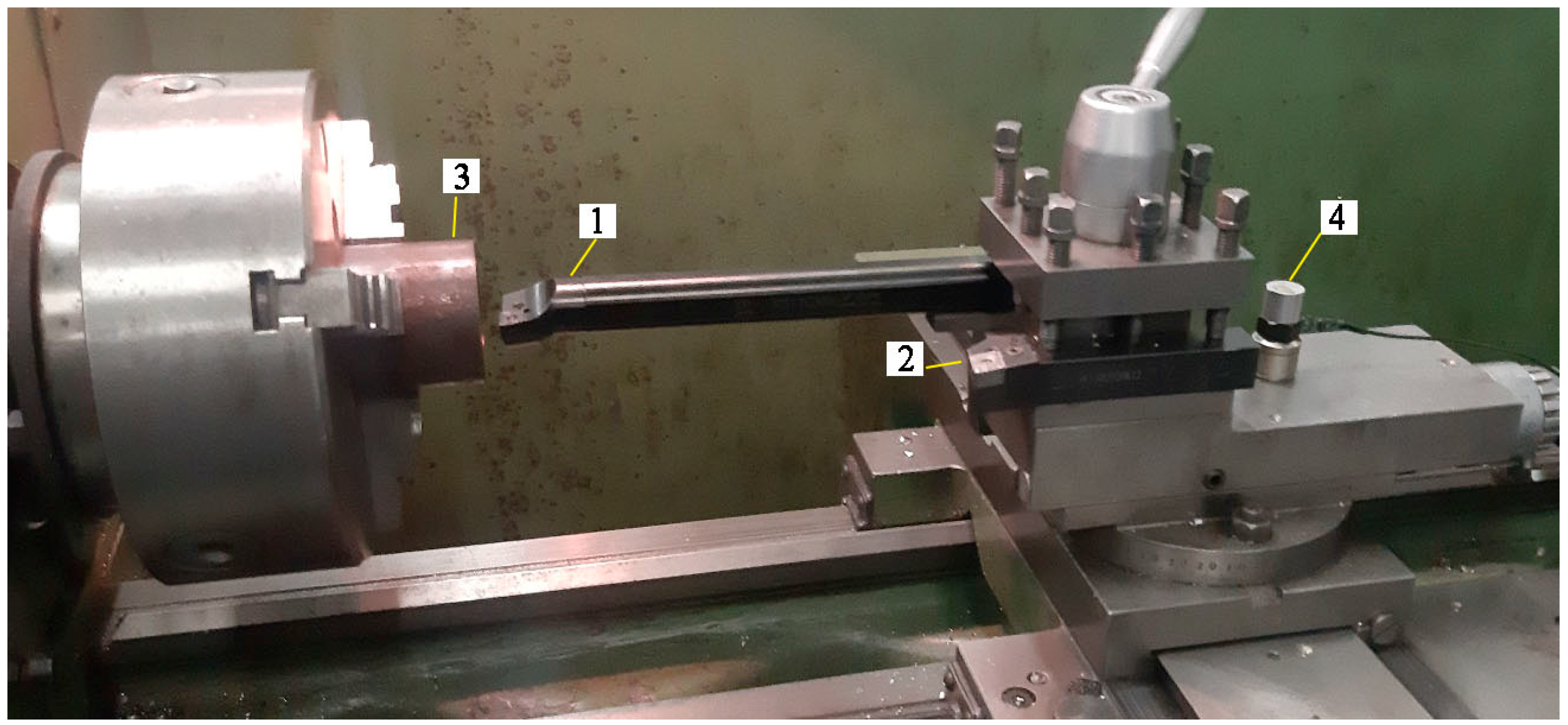
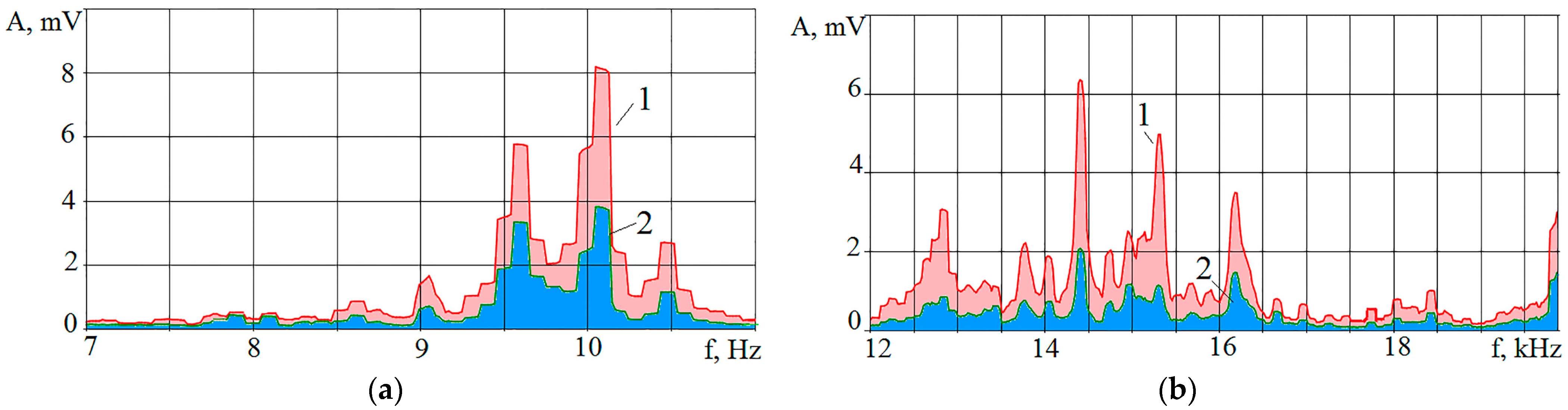
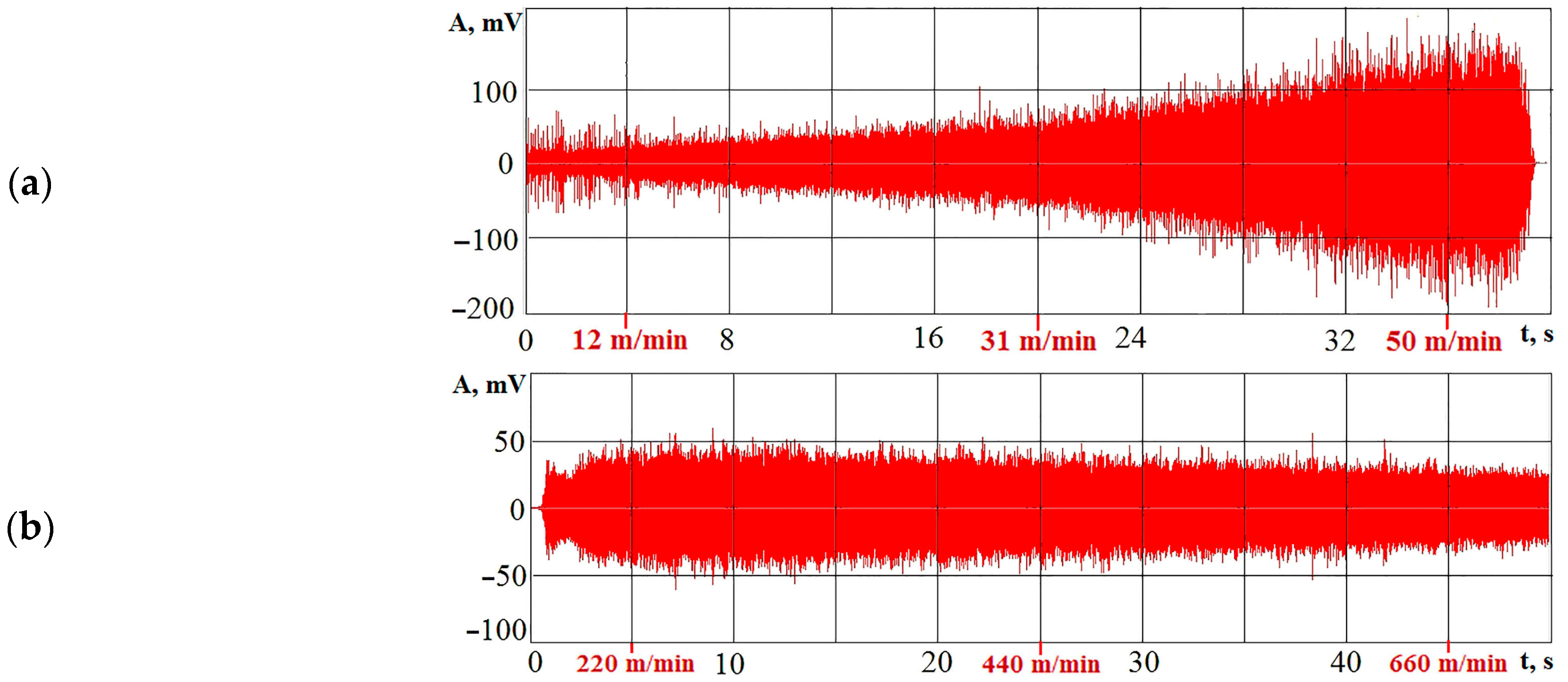
3.1. Results of Studies of AE Signals during Blade Processing

When monitoring blade machining, the most significant interest is in the response of AE signals to changes in the state of the tools. These include wear on cutting edges, chipping, and breakage. In [53], the deformation processes of chips and the surface layer were studied using experimental research and calculations. Figure 7 shows an example of calculating the field of strain rates during chip formation using the Deform program (DEFORM-2D V.8.1). It can be seen that the highest strain rates are located in the vicinity of the conditional shear plane, which is formed from the cutting edge and propagates towards the interface between the surfaces of the workpiece and the formed chip. Tool wear in calculations using the Deform program was simulated by changing the radius of the cutting edge (r).
Its increase leads to an expansion of the region covering areas with significant strain rates, and, hence, to a rise in energy costs for forming these regions. The figure also shows that some areas with different strain rate intensities remain in the surface layer, saturating it with an abundance of dislocation accumulations and microcracks. The exact figure shows the intensity of deformation of the surface layer (εint) along the depth of the layer (δ). The bottom line corresponds to a tool with a radius of 0.02 mm, and the top line corresponds to a tool with a radius of 0.12 mm. It simulates the wear limit. It follows from the graphs that with increasing tool wear, the deformation of the surface layer increases by more than two times. For deeper layers, the difference in the magnitude of deformations is leveled out. Figure 8 shows the results of experiments to determine the intensity of deformations during turning with cutting plates with different degrees of wear. The measurements were carried out using the technique of applying coordinate grids to the cross-sectional surface of the workpiece, the deformation of which was measured after removing the chips [53]. Experiments were carried out for five cutters with different wear. The view of the cutting edge from the back edge for cutters with minimal and maximum wear is shown in the photographs in Figure 8.
Comparing the graphs in Figure 7 and Figure 8, it can be noted that in a full-scale experiment, the deformation values decrease faster; at a depth of 0.2 mm, they are almost invisible. It should be noted that the ratio of the deformation of the surface layer for sharp and excessively worn cutters during full-scale tests was 7–8 times, which significantly exceeds the calculated ratio. This suggests that modeling wear as a cylindrical surface does not correspond to the actual wear shape.
Figure 9 shows the octave spectra of AE signals covering the range up to 11 kHz when turning 41CrS4 steel with the same modes of a sharp (1) and worn (2) tool (photos of the cutter edges are shown in Figure 8). On the graph, it can be noted that in the spectrum of the VA signal, when working with a worn tool, the amplitudes at high frequencies fell, and the amplitudes in the low frequency range increased. This distortion of the AE signal spectrum shape was proposed to be assessed by the amplitude ratio (Kf) in different frequency ranges [47,48,49,50,51,53]. The insert in Figure 9 shows the change in the Kf parameter during turning under the same conditions, but with cutters with different wear. It is essential that the wear was assessed by experimental studies of the surface layer after processing the part [53]. It was not the wear of the cutting edge itself that was plotted horizontally, but the deformation intensity indicator of the surface layer εint. To form the Kf parameter, the ratios of RMS amplitudes in the frequency ranges of 0.75–1.5 kHz and 4.4–15 kHz were used. The choice of frequency ranges for the formation of Kf depends on the natural frequencies of the elastic system of the machine and on the location of the accelerometer and should be based on preliminary experiments. There are no strict boundaries for the selected frequency ranges; they should include areas of natural frequencies with the most remarkable change in amplitudes with increasing wear. The Kf parameter depends less on processing modes if they do not vary too widely (Figure 10). Figure 10a shows the change in Kf with changes in tool wear and cutting speed in a wide range during face turning of NiCr20TiAl steel [54]. Figure 10b shows the difference in the RMS amplitude of the VA signal in the ranges of 0.5–3 kHz and 6–16 kHz and Kf when turning a stepped roller with different cutting depths.
It follows from Figure 9 and Figure 10 that the Kf parameter is quite informative to tool wear, but it significantly depends on the cutting speed. When the cutting speed varies over a wide range, to monitor the condition of the tool at different cutting speeds, it is necessary to have a set of permissible values Kf ≤ [Kf] for each speed range. Variations in cutting depth and tool feed affect Kf significantly less. The situation is simplified, since on modern machines, the cutting speed is maintained in the vicinity of a rational value set in advance. In practice, there should not be such ranges of cutting speed changes as in Figure 10a. Another method of eliminating the impact of a variable cutting speed on the Kf parameter used as a failure criterion may be the use not of Kf itself, but of its relation to the initial value in the absence of wear. Considering the linear form of the dependencies in Figure 10a, this ratio will have an almost constant value over a wide range of cutting speeds.
Another example of changing the Kf parameter is shown for a flat-grinding machine (Figure 3). Parts made of the heat-resistant alloy Inconel 718 were ground with a grinding wheel (electrocorundum) with a solid bond with grain F90 (grinding speed 1800 m/min, double stroke feed 10 μm, processing without lubrication). Figure 11 shows the recording of AE signals during 30 passes.
To assess the change in the Kf parameter, recordings in two frequency ranges, 2–8 and 23–33 kHz, were considered. Figure 12 shows RMS signal amplitudes and Kf for the first and 29th passes.
Figure 11 shows that with each pass of the grinding wheel, the RMS amplitude increases; in Figure 12, you can compare the RMS amplitude for the initial and last passes at different frequency ranges. If we compare the initial and last passes, we can note that by the last pass, the maximum value of the Kf parameter has almost doubled. At this point, burn marks appeared on the surface of the workpiece (Figure 12c).

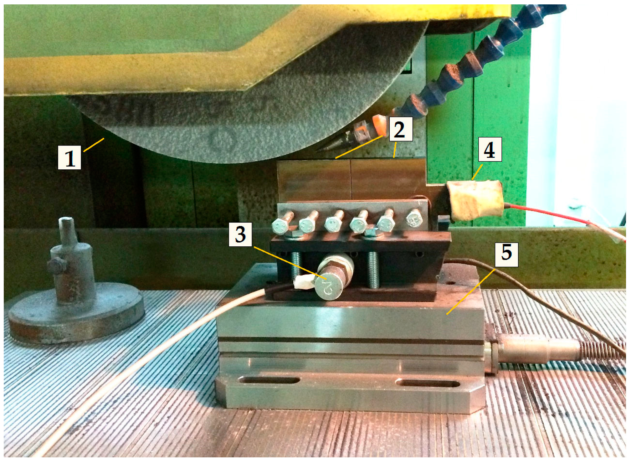
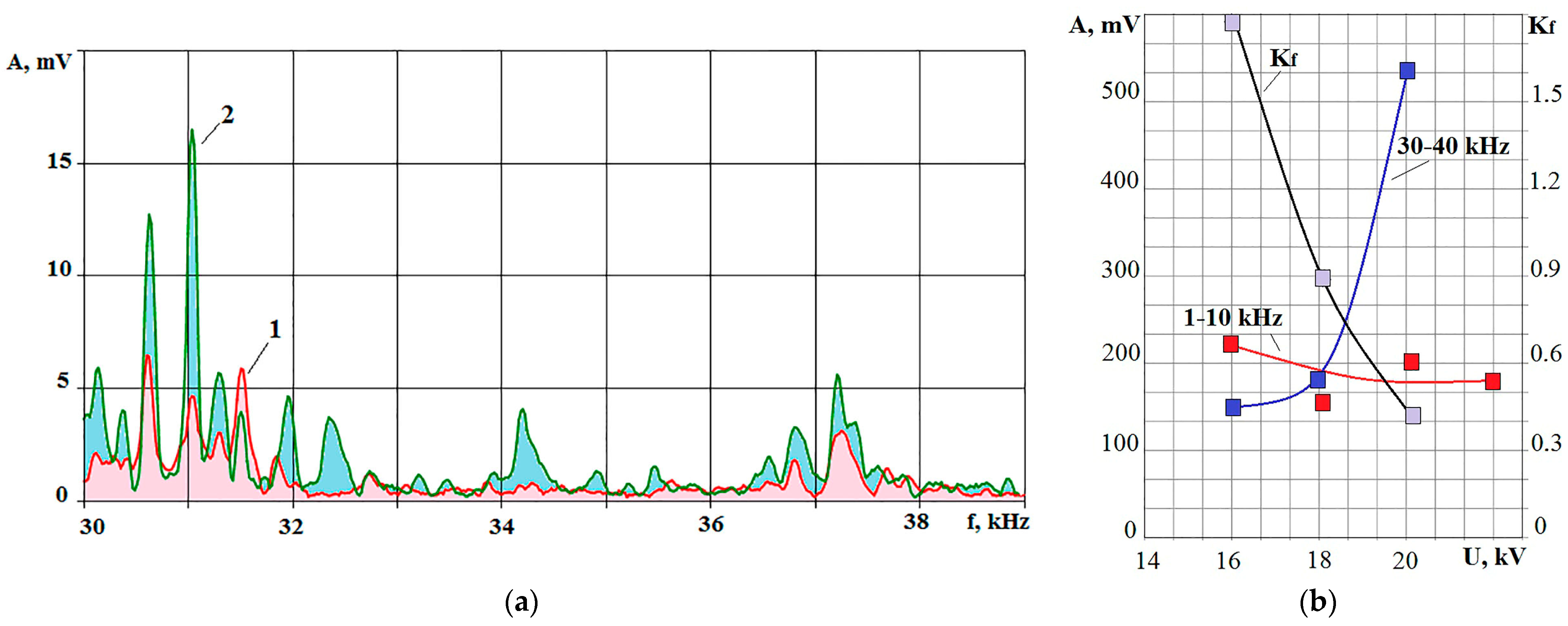
3.2. Results of Studies of AE Signals When Processed Using Concentrated Energy Flows

At first glance, it seems that blade processing and concentrated energy flow processing technologies do not have many common properties. However, similar properties can be found in the behavior of AE signal parameters in these types of processing. Figure 13 shows records of changes in AE signal parameters during the processing of the HG20 (W94K6) alloy on the CUT30P WEDM machine (Figure 6).
Figure 13a shows how the amplitude 1/3 octave spectrum is distorted from the moment the cutting begins until it approaches the moment the wire electrode breaks: the amplitudes at high frequencies decrease, and at low frequencies, they increase. In recordings of the AE signal (Figure 13b) in two frequency ranges, this trend continues. The amplitudes change unevenly, but the noted trend remains. Figure 13c shows how the RMS amplitudes of the AE signal components, the records of which are shown in Figure 13b, and the discrete values of Kf, which are averaged over short periods, change as the moment of electrode break approaches.
If we compare the data in Figure 13 with the blade machining results shown in Figure 9, Figure 10, Figure 11 and Figure 12, the trends in the behavior of the AE signal parameters will be similar in many respects. The central coincidence of the properties of AE signals is that the deterioration of the technological process conditions causes an increase in the Kf parameter, which is the ratio of RMS amplitudes in the low and high frequency ranges. For blade processing, the deterioration of conditions was expressed in increased wear of the cutting tool, and for WEDM processing, as an increase in the concentration of erosion products in the interelectrode gap.
Another method of processing materials with concentrated energy flows is the technology of electron beam doping in a vacuum chamber. Works [49,50,55] described the use of wire waveguides for recording AE signals (Figure 5) from the area of irradiation of workpiece surfaces with electron beams. Figure 14 shows the results of an experiment with irradiation of an M20 alloy [54] with pulses of increasing charging voltage of an electron gun. As the charging voltage increases, the power of the electronic pulse supplied to the processing area, the duration of which was 4 μs, increases. Figure 14a shows the amplitude spectra of the AE signals that accompanied the effects of these pulses on the M20 alloy [54] at charging voltages of 16 kV and 22 kV. The graphs in Figure 14b show the changes in the RMS values of the amplitudes of the AE signals at high and low frequencies during the time, including the moment of the peak value of the AE amplitude at high frequencies. The values of the charging voltage are marked horizontally, which, in this case, is proportional to the heat flow power density.
In the case of electron beam processing with different charging voltages, it is impossible to talk about the deterioration of processing conditions. We can say that the thermal power acting on the surface of the workpiece changed. With a decrease in the power of the heat flow and the preservation of the irradiated area, we can talk about a decrease in the power density qs (the ratio of the power of the heat flow to the area of exposure) and a reduction in the corresponding productivity of the irradiation process. If, conditionally, a drop in power density is taken as a deterioration of conditions (a decrease in productivity), then in the case of electron beam processing, the trend mentioned above of a reduction in Kf will continue with a deterioration in the conditions of the technological process.
A similar change in Kf occurs when the workpiece surface is exposed to laser pulses. If the dimensions of the laser focal spot are kept constant but the power of the radiation generator changes, then the power density of the heat flow will be proportional to the specified power. Figure 15 compares the amplitude spectra of AE signals when a workpiece made of stainless steel AISI 410 is exposed to laser pulses with a power of 60% and 40% of the maximum laser power.
In Figure 15, the amplitude of the AE signal over the entire frequency range at a power of 60% is greater compared to the radiation at a power of 40%. However, it is seen that when the power is reduced by 1.5 times, the decrease in the AE amplitude at high frequencies is significantly greater than the range of lower frequencies. Figure 16 shows the change in RMS amplitudes in the 8 and 16 kHz octave bands when a steel workpiece is exposed to a series of pulses with different power densities.
If, during electron beam processing, an increase in the pulse power density was accompanied by an increase in the amplitude of the AE signal at high frequencies and a barely noticeable decrease in the amplitude in the low frequency range (Figure 14b), then in Figure 15, an increase in amplitudes is visible in both frequency ranges. Since the rate of amplitude growth in the 16 kHz octave is significantly higher than the rate in the 8 kHz octave, the regularity of changes in the Kf parameter corresponds to the previous examples. With a decrease in process performance (quality reduction) due to a decrease in power density, the Kf parameter increases.

4. Results and Discussion

Works [49,53,56] consider the issue of the phase transformation of matter under the impact of laser pulses of different powers. A comparison of existing ideas about the effect of an increase in pulse power density on the transition of a substance to the stages of melting, evaporation, and ionization with the behavior of the parameters of AE signals allowed us to draw a particular conclusion. The meaning of this conclusion is that with an increase in the power density of the thermal effect on a substance, the RMS amplitudes of the AE signal increase in the high frequency range, which is faster than the increase in the RMS amplitudes in the low frequency range. This result is reflected in a drop in the Kf parameter with an increased heat flow power density. This conclusion was confirmed by the results of experiments with EDM processing and electron beam processing.
For example, Figure 13b shows records of changes in the components of the AE signal in the high and low frequency ranges during the WEDM processing of the HG20 alloy. The recording was carried out from the very beginning of cutting until the wire electrode broke. The reason for the break was that erosion products gradually accumulated in the gap between the electrodes, which absorbed part of the energy of the discharge pulses. As a result, the valuable power density decreased and the proportion of evaporated substance decreased. In this case, melted material accumulated on the electrodes, and the gap between the electrodes was reduced, causing a short circuit. Subsequent heating of the electrodes led to a loss of strength of the wire electrode and its breakage. Figure 13c shows how the Kf parameter changed by the time of the break. If the machine had an acoustic monitoring system, it would have been possible to prevent electrode breakage by promptly stopping its feed and carrying out relaxation to remove erosion products from the gap.
The situation with electron beam processing is very similar to what was observed when exposed to laser pulses with different power densities (Figure 14b). The difference lies in the heat flow carriers. An increase in the power density of the electron flow causes increased evaporation of the doping coating [53,54,55,56,57]. To prevent its complete evaporation, it is necessary to limit the discharge voltage of the electron gun. Thus, an increase in the discharge voltage corresponds to a rise in the power density of the heat flow and is accompanied by an increase in the proportion of evaporated material. Evaporation processes cause an increase in the energy of acoustic radiation at high frequencies, which determines the drop in the Kf parameter shown in Figure 14b. The ability to monitor the parameters of AE signals is beneficial when debugging new technological processes with unstudied properties of doping coating materials [49,50,57].
If the connection between the features of changes in the parameters of AE signals and changes in power density and, accordingly, the proportion of evaporated material during processing with concentrated energy flows is clear, then the connection between acoustic parameters and wear of a blade tool needs an explanation. In this case, there are no thermal pulses, the power density of which can be associated with changes in the parameters of the AE signals. From the theory of spectral analysis of pulse signals, it is known that the frequency of the upper limit of the decomposition of a pulse signal into a spectrum containing the bulk of the pulse energy is inversely proportional to the pulse duration [58]. The mechanisms of changing the time of pulses during cutting can be different. The main ones include the following:
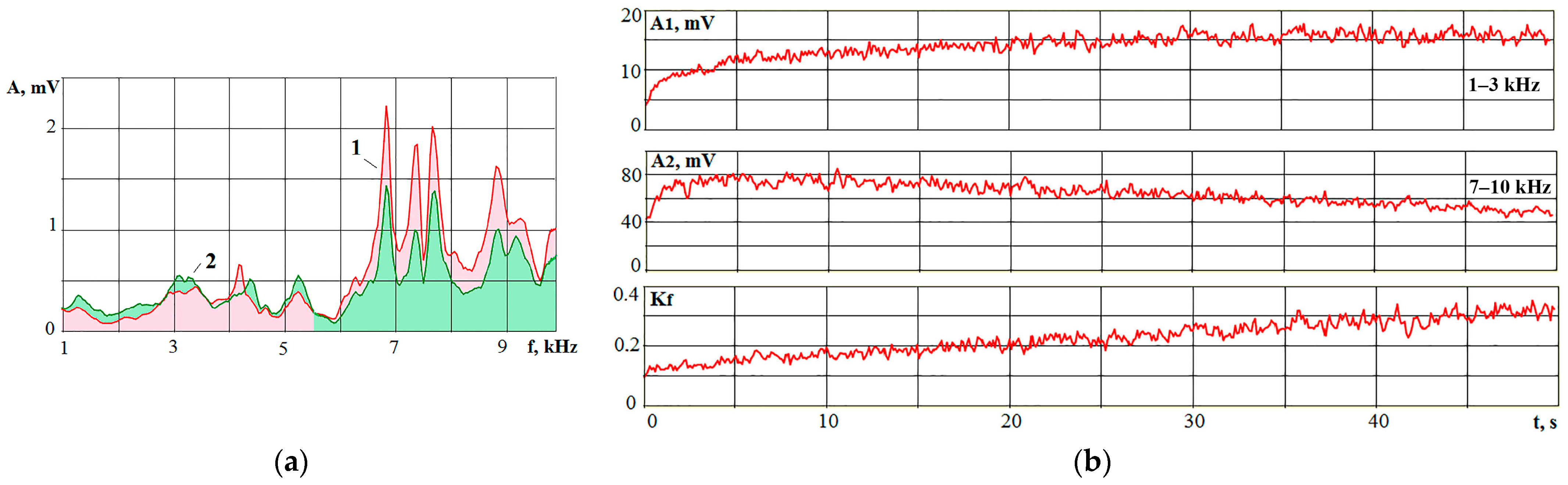
  • An increase in the load in the contact of the tool with the treated surface is accompanied by an increase in friction powers, causing the dissipation of vibrational energy, which is especially noticeable in the high frequency range.
  • An increase in frictional powers between the surfaces of the tool and the workpiece causes heating of the surfaces. This can lead to a decrease in the mechanical properties of processed material, which reduces the proportion of brittle fracture in favor of the viscous mechanism during chip formation. Brittle cracks are characterized by a high speed of crack movement and short pulses that create amplitude spectra propagating into the high frequency range. Viscous cracks have a significantly lower rate of development and form longer pulses, producing smaller amplitudes at high frequencies.
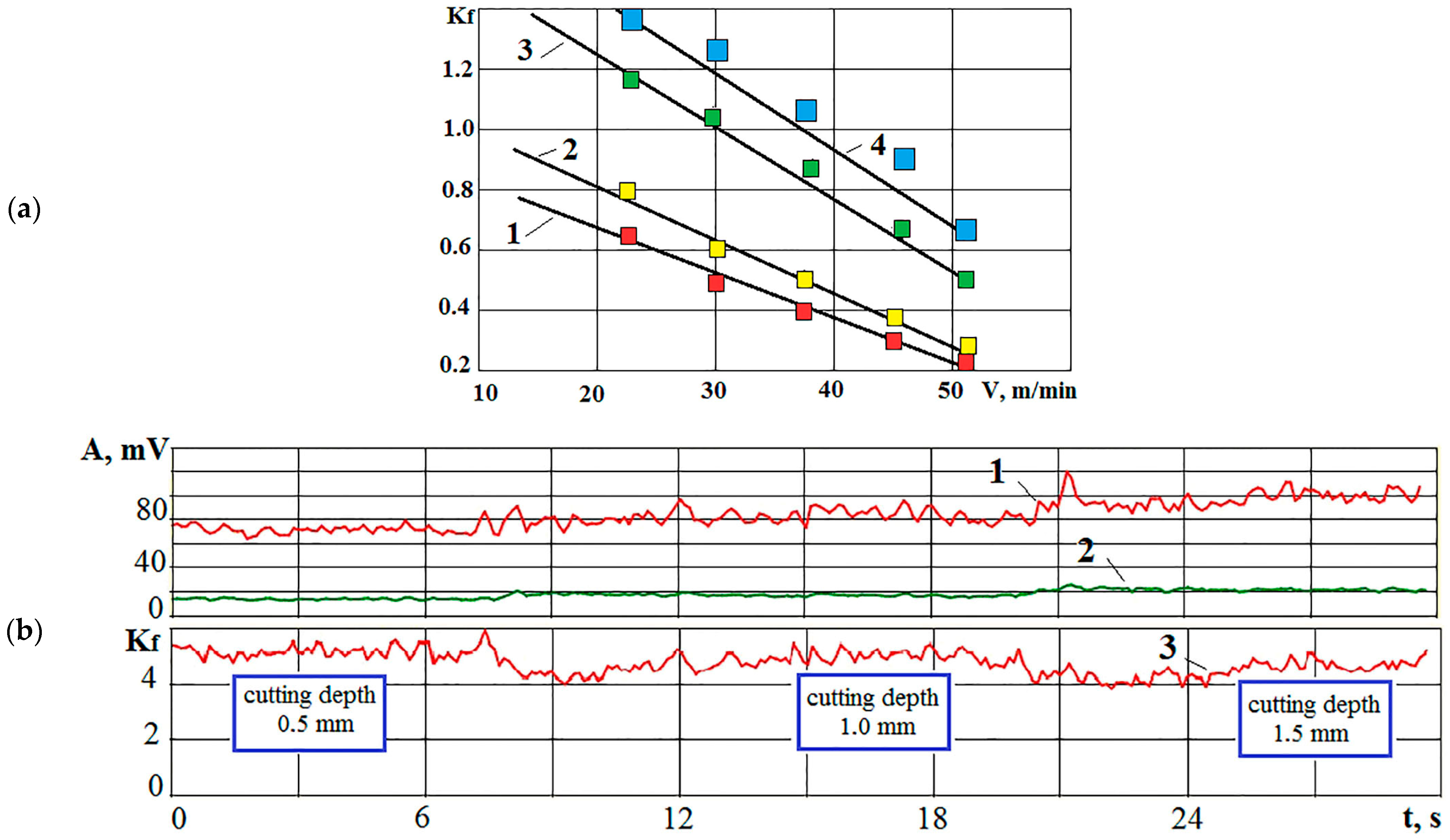
  • Changes in the rigidity of the elements of the elastic system, including the tool, the part, and mechanisms for their mounting. An increase in cutting powers during wear of the cutting edge can cause mobility in the joints of parts, leading to an increase in the duration of pulses accompanying the formation of chip elements.
To substantiate the first mechanism, Figure 17 shows how the amplitude of the AE signal changes in different octave bands when the grinding wheel on a flat-grinding machine (Figure 3) comes into contact with the workpiece. In Figure 17, the value δ shows a decrease in the initial amplitude A. Their ratio Δ as a percentage reflects the impact of frictional interaction on the AE signal. When the tool and the workpiece come into contact, the interaction of the grinding wheel grains is present, and friction does not have time to form yet. Still, at subsequent moments, normal loads and a corresponding friction power arise in the contact. This immediately affects the amplitude of the AE signal, but in different frequency ranges, and the result of a decrease in amplitude is different.
Figure 17 shows the percentage reduction in RMS of AE amplitudes for seven octaves. For the lower three octaves, there were no noticeable changes, and friction did not affect the AE signals in these frequency ranges. Further, the percentage decrease in amplitude increased from octave to octave. In the 32 kHz octave band, the amplitude dropped by 82%. The shown change in the composition of the acoustic signal indicates that in the state of close contact between the tool and the workpiece, the pulses of interaction between the grinding grains and the workpiece become longer. As the contact density increases, surface irregularities transform into a state close to all-round compression, which prevents the formation of brittle cracks, and the pulses become longer. In this case, the interaction energy is distributed over a more extended period, which reduces the power density.
The second mechanism is associated with a temperature change that increases with friction. An increase in temperature affects the mechanical properties of materials, such as hardness and elastic modulus. In metals, an accelerated decline in mechanical properties begins in the region of temperatures 0.5 from the melting temperature [59]. Changes in the parameters of the AE signals when the temperature of the tool and workpiece changes under the impact of friction powers can be traced when turning steel workpieces at different speeds. Figure 18 shows recordings of the high-frequency AE signal during face turning at constant speeds with an increasing cutting speed due to transverse feed towards the periphery. Figure 18a shows a recording of a VA signal in the frequency range of 7–10 kHz when turning NiCr20TiAl steel [54] at relatively low speeds. Figure 18b shows a similar record, but at increased cutting speeds of 41CrS4steel.
Figure 18a shows that with an increasing cutting speed, the signal amplitude increases almost linearly. Steel NiCr20TiAl [54] is a heat-resistant steel, in which, with a significant (up to 700°) increase in temperature, the mechanical properties change within 10–20%. Relatively low cutting speeds and heat-resistant properties made it possible to maintain an almost linear dependence of the amplitude on the relative rate in contact.
In Figure 18b, when turning conventional alloy steel at increasing speeds, the picture changes radically. We can talk about an increase in amplitude only at the initial moment. A further increase in cutting speed causes a decrease in the amplitude of the AE signal. For steel 41CrS4, with increasing temperature, the mechanical properties can decrease several times. As the cutting speed approached 600 m/min, red chips were observed. Figure 19 compares the spectra of the AE signal at the start of cutting at a speed of about 200 m/min (1) and at the end of the pass, when the cutting speed exceeds 660 m/min (2). In the frequency range up to 6 kHz, the amplitudes in the spectrum for high rates are slightly higher than the amplitudes of the spectrum for low rates. However, at high rates, the amplitudes for the frequency range above 6 kHz become significantly lower. In the entries in Figure 18b, the Kf coefficients varied, as shown in Figure 19b. The frequency range of 1–3 kHz was used as the low frequency range.
Thus, we can conclude that the increase in friction powers and increased heat generation accompanying the wear of cutting tools determine the drop in the amplitudes of acoustic signals at high frequencies. These processes help to reduce the proportion of brittle fracture in favor of viscous fracture, which is characterized by the spread of viscous cracks that form longer pulses. Long pulses correspond to lower power densities.
From the previously given list of mechanisms affecting the duration of pulses during chip formation, it remains to be considered the last factor that can cause changes in the parameters of the AE signals, similar to tool wear. We are talking about the rigidity of the technological system, including the tool, the workpiece with the device, and the machine itself. With the automated installation of workpieces and tools in the working position with the help of manipulators, random deviations from the intended mounting mode (misalignment and ingress of chips) may occur. These deviations affect the static and dynamic rigidity of the technological system, which affect the quality of processing even with a sharp tool. These situations can cause changes in the parameters of the AE signals, similar to the effects of tool wear. Figure 20 shows the spectra of the AE signal when turning 41CrS4 steel, where one of the mounting screws was clamped under the standards, and the mounting of the other screw was insufficient.
In Figure 20a, it can be seen that the AE amplitude for almost all frequencies up to 5 kHz increased when the cutter mounting was loosened compared to normal cutting. Above 15 kHz (Figure 20b), the AE amplitude for the case of loosened mounting, on the contrary, becomes lower than the amplitude with a normal clamp. RMS amplitudes in the frequency ranges of 0.5–3 kHz and 6–10 kHz were used to calculate Kf. With normal mounting, the Kf fluctuated around 0.8, and when the mounting was loosened, it approached 3. Thus, Kf grew more than three times. If we take the range of 15–25 kHz as high frequencies, the value of Kf with a loosened mount will increase by five times. Figure 20 shows photos of chips obtained with different qualities of mounting of the turning tool.
The photographs in Figure 21 show that loose mounting of the cutter leads to difficulties in the chip-forming process. There is tearing and breakouts on the chips, and the stability of their formation is disturbed. At the moment of formation of the chip element, it is essential that the power pulse must act for a short period of time on a minimum area so that the impact mode is realized in the form of a power pulse for a short period. Then, brittle cracks are formed, accompanied by AE with a large amplitude at a high frequency. Low mobility in the mounting stretches the impact pulse (reduces power density), creating chip elements using viscous cracks. The presence of loose joints can be challenging to identify by assessing the dynamic characteristics of an elastic system, since mobility in a joint can only manifest itself under a disturbing impact with an amplitude exceeding a specific threshold value. If there is a danger of insufficient mounting of elements of the elastic system, then it is better to identify it at the initial processing stage. This can be performed by comparing the average Kf values with the typical value for a given operation.
During the boring operation, AE signals were also recorded to compare the acoustic effects with those obtained during turning. Figure 22 shows the spectra of AE signals recorded when boring a hole in a workpiece made of steel 40 (Ø 40, depth 1 mm, feed 0.15 mm/rev). Figure 22a shows spectra for up to 5 kHz, and Figure 22b shows the range of 5–25 kHz. Number 1 indicates spectra, recordings and photos during boring with normal clamping of the boring tool, and number 2 indicates when one screw is loosened. Spectrum 2 in Figure 22a contains narrow amplitude peaks characteristic of the self-oscillating mode, which forms the low quality of the boring surface (photo 2 in Figure 22b). By analogy with Figure 20b, Figure 22b shows that at high frequencies, when the mount is loosened, the amplitudes drop sharply over the entire frequency range. The insert in Figure 21a shows examples of recordings of VA signals in the range of 0.6–1.6 kHz, where the negative impact of poor tool mounting can be seen.
Changes in the conditions for mounting the boring tool also significantly affected the Kf indicator, which changed by an order of magnitude, even when choosing different frequency ranges for which the effective amplitudes were determined (see Table 2).
To determine the Kf values in Table 2, two options were used as the high frequency range. The Kf values were different, but the ratio between Kf with normal and loose mounting was almost the same.

5. Conclusions

  • Studies of the relationship of AE parameters with the features of various technological processes have shown that these parameters can be used in the conditions of automated production as a supplement to the existing monitoring tools or separately.
  • As a result of studies of some technological processes, including blade processing and processing with concentrated energy flows, features of changes in the spectral composition of acoustic signals, a characteristic of many technological processes using different principles of energy impact on the material being processed, were established.
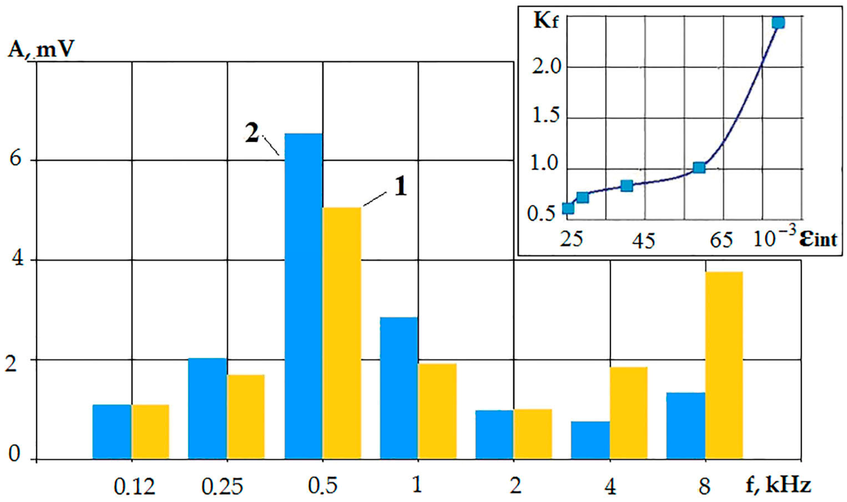
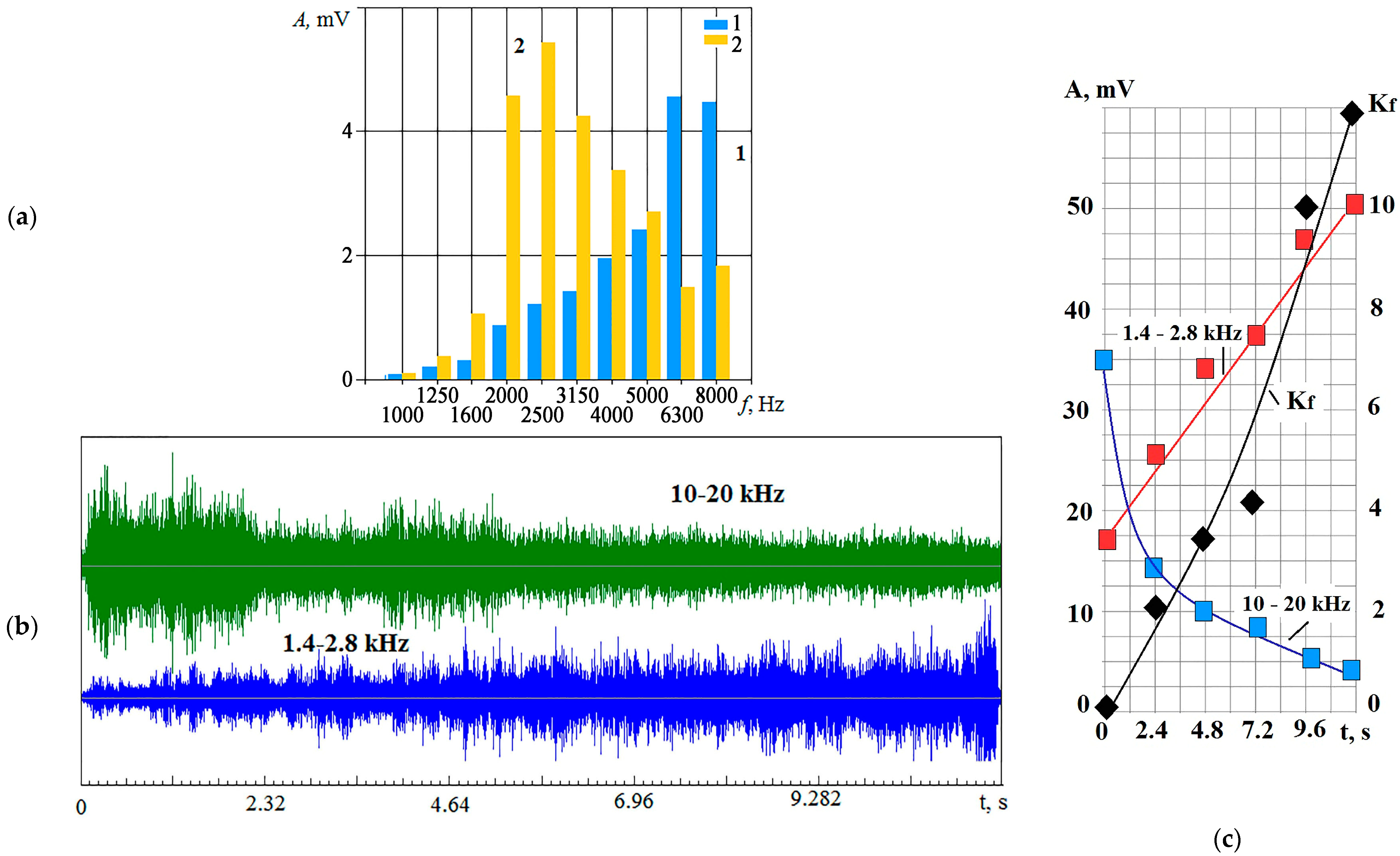
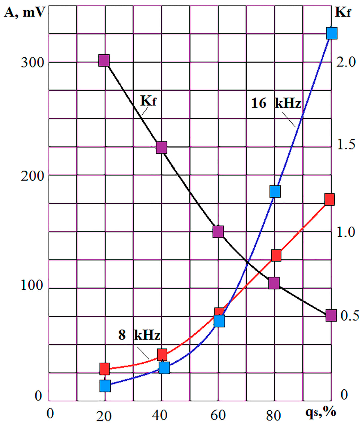
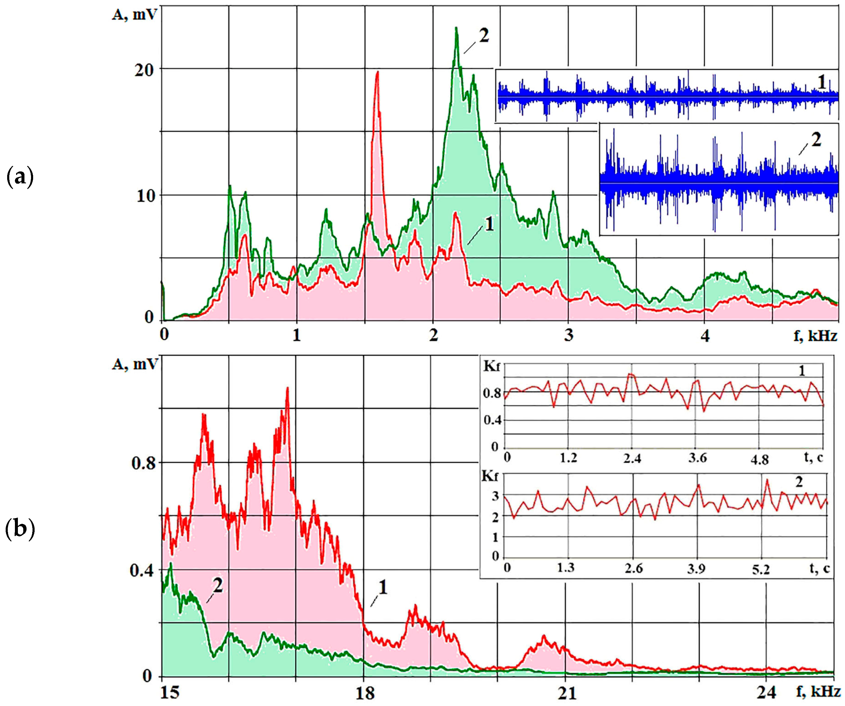
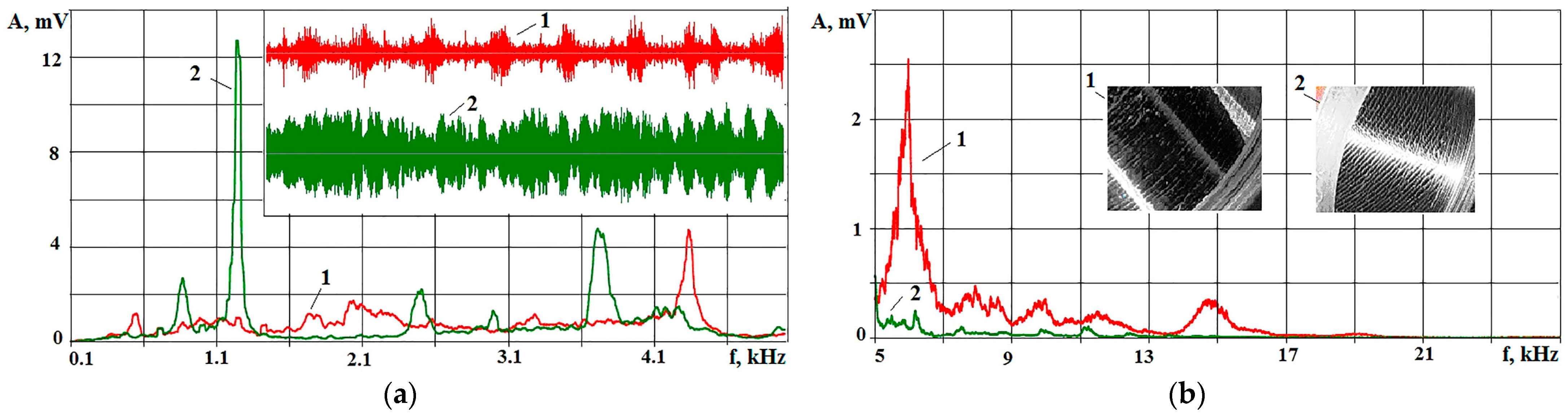
  • It was found that the main reason for the impact on changes in the characteristics of the acoustic signal is the change in the power density of the energy impact on the workpiece material. The power density, defined as the impact power per unit of surface, changes with a change in the power of the energy source, with an increase in the impact surface area, and with the extension of the time of the duration of the energy pulses accompanying the treatment. A decrease in power density entails a drop in the amplitude of the high-frequency component of acoustic signals compared to the low-frequency component.
  • For practical use of acoustic signal parameters, the ratio of RMS amplitudes of acoustic signals in the low and high frequency ranges can be controlled. An increase in this ratio indicates that the pulses of energy action on the material have become smaller in amplitude or have become more stretched over time. That is, changes in the technological process led to a drop in the power density of the impact on the material. In laser processing, this is associated with a shift in the focal plane. In WEDM, it is associated with an increase in the concentration of erosion products. In blade processing, it is associated with an increase in tool wear, an increase in the area of impact of the cutting edge and, accordingly, the transition to a viscous mechanism of crack formation when the chip elements are shifted.

Author Contributions

Conceptualization, S.N.G.; methodology, M.P.K.; software, A.N.P. and Y.A.M.; validation, Y.A.M.; formal analysis, V.D.G. and Y.A.M.; investigation, M.P.K. and A.N.P.; resources, A.N.P.; data curation, M.P.K. and V.D.G.; writing—original draft preparation, S.N.G.; writing—review and editing, M.P.K.; visualization, A.N.P. and Y.A.M.; supervision, S.N.G. and M.P.K.; project administration, M.P.K.; funding acquisition, S.N.G. All authors have read and agreed to the published version of the manuscript.

Funding

This work was supported financially by the Ministry of Science and Higher Education of the Russian Federation (project No. FSFS-2021-0003).

Institutional Review Board Statement

Not applicable.

Informed Consent Statement

Not applicable.

Data Availability Statement

The data presented in this study are available on request from the corresponding author.

Acknowledgments

The study was carried out on the equipment at the Center of Collective Use of MSUT “STANKIN”, supported by the Ministry of Higher Education of the Russian Federation (project No. 075-15-2021-695 from 26 July 2021, unique identifier RF 2296.61321X0013).

Conflicts of Interest

The authors declare no conflicts of interest.

References

  1. Tran, M.Q.; Liu, M.K. Chatter Identification in End Milling Process Based on Cutting Force Signal Processing. IOP Conf. Ser. Mater. Sci. Eng. 2019, 654, 012001. [Google Scholar] [CrossRef]
  2. Barakat, M.; Lefebvre, D.; Khalil, M.; Druaux, F.; Mustapha, O. Parameter selection algorithm with self-adaptive growing neutral network classifier for diagnosis issues. Int. J. Mach. Learn. Cybern. 2013, 4, 217–233. [Google Scholar] [CrossRef]
  3. Kurpiel, S.; Zagórski, K.; Cieślik, J.; Skrzypkowski, K.; Brostow, W. Evaluation of the Vibration Signal during Milling Vertical Thin-Walled Structures from Aerospace Materials. Sensors 2023, 23, 6398. [Google Scholar] [CrossRef] [PubMed]
  4. Stavropoulos, P.; Chantzis, D.; Doucas, C.; Papacharalampopoulos, A.; Chryssolouris, G. Monitoring and control of manufacturing processes: A review. Proc. CIRP 2013, 8, 421–425. [Google Scholar] [CrossRef]
  5. Test & Measurement Pressure—Measurement Equipment for Demanding T&M Applications. Available online: www.kistler.com (accessed on 20 November 2023).
  6. Chai, M.; Hou, X.; Zhang, Z.; Duan, Q. Identification and prediction of fatigue crack growth under different stress ratios using acoustic emission data. Int. J. Fatigue 2022, 160, 106860. [Google Scholar] [CrossRef]
  7. Komanduri, R.; Hou, Z.B. A review of the experimental techniques for the measurement of heat and temperatures generated in some manufacturing processes and tribology. Tribol. Int. 2001, 34, 653–682. [Google Scholar] [CrossRef]
  8. Bagavathiappan, S.; Lahiri, B.B.; Saravanan, T.; Philip, J.; Jayakumar, T. Infrared thermography for condition monitoring—A review. Infrared Phys. Technol. 2013, 60, 35–55. [Google Scholar] [CrossRef]
  9. Jadin, M.S.; Taib, S. Recent progress in diagnosing the reliability of electrical equipment by using infrared thermography. Infrared Phys. Technol. 2012, 55, 236–245. [Google Scholar] [CrossRef]
  10. Utami, N.Y.; Tamsir, Y.; Pharmatrisanti, A.; Gumilang, H.; Cahyono, B.; Siregar, R. Evaluation condition of transformer based on infrared thermography results. In Proceedings of the 2009 IEEE 9th International Conference on the Properties and Applications of Dielectric Materials, Harbin, China, 19–23 July 2009; pp. 1055–1058. [Google Scholar] [CrossRef]
  11. Huda, A.S.N.; Taib, S. Suitable features selection for monitoring thermal condition of electrical equipment using infrared thermography. Infrared Phys. Technol. 2013, 61, 184–191. [Google Scholar] [CrossRef]
  12. Reigosa, D.D.; Guerrero, J.M.; Diez, A.B.; Briz, F. Rotor Temperature Estimation in Doubly-Fed Induction Machines Using Rotating High-Frequency Signal Injection. IEEE Trans. Ind. Appl. 2017, 53, 3652–3662. [Google Scholar] [CrossRef]
  13. Zhiming, Z.; Ji, F.; Guan, Y.; Xu, J.; Yuan, X. Method and experiment of Temperature Collaborative Monitoring based on Characteristic Points for tilting pad bearings. Tribol. Int. 2017, 114, 77–83. [Google Scholar] [CrossRef]
  14. Visnadi, L.B.; De Castro, H.F. Influence of bearing clearance and oil temperature uncertainties on the stability threshold of cylindrical journal bearings. Mech. Mach. Theory 2019, 134, 57–73. [Google Scholar] [CrossRef]
  15. Dutta, S.; Pal, S.; Mukhopadhyay, S.; Sen, R. Application of digital image processing in tool condition monitoring: A review. CIRP J. Manuf. Sci. Technol. 2013, 6, 212–232. [Google Scholar] [CrossRef]
  16. Wong, Y.; Nee, A.; Li, X.; Reisdorj, C. Tool condition monitoring using laser scatter pattern. J. Mater. Process. Technol. 1997, 63, 205–210. [Google Scholar] [CrossRef]
  17. Castejon, M.; Alegre, E.; Barreiro, J. On-line tool wear monitoring using geometric descriptors from digital images. Int. J. Mach. Tools Manuf. 2007, 47, 1847–1853. [Google Scholar] [CrossRef]
  18. Peeters, C.; Antoni, J.; Helsen, J. Blind filters based on envelope spectrum sparsity indicators for bearing and gear vibration-based condition monitoring. Mech. Syst. Signal Process. 2020, 138, 106556. [Google Scholar] [CrossRef]
  19. Yu, G.; Lin, T.; Wang, Z.; Li, Y. Time-Reassigned Multisynchrosqueezing Transform for Bearing Fault Diagnosis of Rotating Machinery. IEEE Trans. Ind. Electron. 2021, 68, 1486–1496. [Google Scholar] [CrossRef]
  20. Saucedo-Dorantes, J.; Delgado-Prieto, M.; Osornio-Rios, R.; Romero-Troncoso, R. Spectral analysis of nonlinear vibration effects produced by worn gears and damaged bearing in electromechanical systems: A condition monitoring approach. In Nonlinear Structural Dynamics and Damping; Jauregui, J.C., Ed.; Springer: New York, NY, USA, 2019; pp. 293–320. [Google Scholar] [CrossRef]
  21. Li, C.; Sanchez, R.V.; Zurita, G.; Cerrada, M.; Cabrera, D.; Vásquez, R.E. Gearbox fault diagnosis based on deep random forest fusion of acoustic and vibratory signals. Mech. Syst. Signal Process. 2016, 76–77, 283–293. [Google Scholar] [CrossRef]
  22. Wang, L.; Shao, Y. Fault feature extraction of rotating machinery using a reweighted complete ensemble empirical mode decomposition with adaptive noise and demodulation analysis. Mech. Syst. Signal Process. 2020, 138, 106545. [Google Scholar] [CrossRef]
  23. Bai, C.; Ganeriwala, S.S.; Sawalhi, N. A rational basis for determining vibration signature of shaft/coupling misalignment in rotating machinery. In Rotating Machinery, Vibro-Acoustics & Laser Vibrometry; Di Maio, D., Ed.; Springer: New York, NY, USA, 2019; Volume 7, pp. 207–217. [Google Scholar] [CrossRef]
  24. Zhou, L.; Duan, F.; Mba, D. Wireless acoustic emission transmission system designed for fault detection of rotating machine. In Advanced Technologies for Sustainable Systems; Bahei-El-Din, Y., Hassan, M., Eds.; Springer: Cham, Switzerland, 2017; pp. 201–207. [Google Scholar] [CrossRef]
  25. Crivelli, D.; Hutt, S.; Clarke, A.; Borghesani, P.; Peng, Z.; Randall, R. Condition Monitoring of Rotating Machinery with Acoustic Emission: A British–Australian Collaboration. In Asset Intelligence through Integration and Interoperability and Contemporary Vibration Engineering Technologies. Lecture Notes in Mechanical Engineering; Mathew, J., Lim, C., Ma, L., Sands, D., Cholette, M., Borghesani, P., Eds.; Springer: Cham, Switzerland, 2019; pp. 119–128. [Google Scholar] [CrossRef]
  26. Kozochkin, M.P.; Porvatov, A.N. Mechanical measurements: Estimation of uncertainty in solving multiparameter diagnostic problems. Meas. Tech. 2015, 58, 173–178. [Google Scholar] [CrossRef]
  27. Liptai, R.G.; Dunegan, H.L.; Tatro, C.A. Acoustic Emission Generated During Phase Transformations in Metals and Alloys. Int. J. Nondestruct. Test. 1969, 1, 213–221. Available online: https://scholar.google.com/scholar_lookup?title=Acoustic+Emission+Generated+During+Phase+Transformations+in+Metals+and+Alloys&author=Liptai,+R.G.&author=Dunegan,+H.L.&author=Tatro,+C.A.&publication_year=1969&journal=Int.+J.+Nondestruct.+Test.&volume=1&pages=213%E2%80%93221 (accessed on 27 December 2023).
  28. Shea, M.M. Amplitude distribution of acoustic emission produced during martensitic transformation. Mater. Sci. Eng. 1984, 64, L1–L6. [Google Scholar] [CrossRef]
  29. Speich, G.R.; Fisher, R.M. Acoustic Emission During Martensite Formation. In Acoustic Emission; ASTM. STP505; ASTM International: West Conshohocken, PA, USA, 1972; pp. 140–151. [Google Scholar] [CrossRef]
  30. Ono, K.; Schlothauer, T.S.; Koppenaal, T.J. Acoustic emission from ferrous martensites. J. Acoust. Soc. Am. 1974, 55, 367. [Google Scholar] [CrossRef]
  31. Speich, L.R.; Schwoeble, A.J. Acoustic emission during phase transformation in steel. In Monitoring Structural Integrity by Acoustic Emission; ASTM. STP571; ASTM International: West Conshohocken, PA, USA, 1975; pp. 40–58. [Google Scholar] [CrossRef]
  32. Bernard, J.; Boinet, M.; Chatenet, M.; Dalard, F. Contribution of the Acoustic Emission Technique to Study Aluminum Behavior in Aqueous Alkaline Solution. Electrochem. Solid-State Lett. 2005, 8, E53–E55. [Google Scholar] [CrossRef]
  33. Kuznetsov, D.M.; Smirnov, A.N.; Syroeshkin, A.V. New Ideas and Hypotheses: Acoustic emission on phase transformations in aqueous medium. Russ. J. Gen. Chem. 2008, 78, 2273–2281. [Google Scholar] [CrossRef]
  34. Builo, S.I.; Kuznetsov, D.M. Acoustic-emission testing and diagnostics of the kinetics of physicochemical processes in liquid media. Russ. J. Nondestruct. Test. 2010, 46, 684–689. [Google Scholar] [CrossRef]
  35. Kuznetsov, D.M.; Builo, S.I.; Ibragimova, J.A. Correlation evaluation of the acoustic emission’s method the tool of exo salvation kinetic’s research. Chem. Technol. 2011, 6, 112–114. Available online: https://www.tsijournals.com/articles/correlation-evaluation-of-the-acoustic-emissions-method-the-tool-of-exo-solvation-kinetiks-research.pdf (accessed on 20 November 2023).
  36. Bashkov, O.V.; Bashkova, T.I.; Popkova, A.A.; Hu, M. Study of the kinetics of fatigue fracture of titanium alloys by acoustic emission. Mod. Mater. Technol. 2013, 1, 020–025. Available online: https://scholar.google.com/scholar_lookup?title=Study+of+the+kinetics+of+fatigue+fracture+of+titanium+alloys+by+acoustic+emission&author=Bashkov,+O.V.&author=Bashkova,+T.I.&author=Popkova,+A.A.&author=Hu,+M.&publication_year=2013&journal=Mod.+Mater.+Technol.&volume=1&pages=020%E2%80%93025 (accessed on 27 December 2023).
  37. Koranne, A.J.; Kachare, J.A.; Jadhav, S.A. Fatigue crack analysis using acoustic emission. Int. Res. J. Eng. Technol. 2017, 4, 1177–1180. Available online: https://www.irjet.net/archives/V4/i1/IRJET-V4I1211.pdf (accessed on 20 November 2023).
  38. Aggelis, D.G.; Kordatos, E.Z.; Matikas, T.E. Monitoring of metal fatigue damage using acoustic emission and thermography. J. Acoust. Emiss. 2011, 29, 113–122. Available online: https://scholar.google.com/scholar_lookup?title=Monitoring+of+metal+fatigue+damage+using+acoustic+emission+and+thermography&author=Aggelis,+D.G.&author=Kordatos,+E.Z.&author=Matikas,+T.E.&publication_year=2011&journal=J.+Acoust.+Emiss.&volume=29&pages=113%E2%80%93122 (accessed on 27 December 2023).
  39. Othman, M.S.; Nuawi, M.Z.; Mohamed, R. Experimental comparison of vibration and acoustic emission signal analysis using kurtosis-based methods for induction motor bearing condition monitoring [Eksperymentalne porównanie drgań i analizy sygnałów emisji akustycznej do monitorowania stanu łożysk]. Prz. Elektrotech. 2016, 92, 208–212. [Google Scholar] [CrossRef]
  40. Vereschaka, A.; Tabakov, V.; Grigoriev, S.; Sitnikov, N.; Oganyan, G.; Andreev, N.; Milovich, F. Investigation of wear dynamics for cutting tools with multilayer composite nanostructured coatings in turning constructional steel. Wear 2019, 420–421, 17–37. [Google Scholar] [CrossRef]
  41. Holguín-Londoño, M.; Cardona-Morales, O.; Sierra-Alonso, E.F.; Mejia-Henao, J.D.; Orozco-Gutiérrez, Á.; Castellanos-Dominguez, G. Machine Fault Detection Based on Filter Bank Similarity Features Using Acoustic and Vibration Analysis. Math. Probl. Eng. 2016, 2016, 7906834. [Google Scholar] [CrossRef]
  42. Jena, D.; Panigrahi, S. Automatic gear and bearing fault localization using vibration and acoustic signals. Appl. Acoust. 2015, 98, 20–33. [Google Scholar] [CrossRef]
  43. Delgado-Arredondo, P.A.; Morinigo-Sotelo, D.; Osornio-Rios, R.A.; Avina-Cervantes, J.G.; Rostro-Gonzalez, H.; de Jesus Romero-Troncoso, R. Methodology for fault detection in induction motors via sound and vibration signals. Mech. Syst. Signal Proc. 2017, 83, 568–589. [Google Scholar] [CrossRef]
  44. Stief, A.; Ottewill, J.R.; Orkisz, M.; Baranowski, J. Two stage data fusion of acoustic, electric and vibration signals for diagnosing faults in induction motors. Elektron. Elektrotech. 2017, 23, 19–24. [Google Scholar] [CrossRef]
  45. Frigieri, E.P.; Brito, T.G.; Ynoguti, C.A.; Paiva, A.P.; Ferreira, J.R.; Balestrassi, P.P. Pattern recognition in audible sound energy emissions of AISI 52100 hardened steel turning: A MFCC-based approach. Int. J. Adv. Manuf. Technol. 2017, 88, 1383–1392. [Google Scholar] [CrossRef]
  46. Grigoriev, S.N.; Kozochkin, M.P.; Porvatov, A.N.; Volosova, M.A.; Okunkova, A.A. Electrical discharge machining of ceramic nanocomposites: Sublimation phenomena and adaptive control. Heliyon 2019, 5, e02629. [Google Scholar] [CrossRef]
  47. Kozochkin, M.P. Study of Frictional Contact during Grinding and Development of Phenomenological Model. J. Frict. Wear 2017, 38, 333–337. [Google Scholar] [CrossRef]
  48. Grigoriev, S.N.; Martinov, G.M. Research and development of a cross-platform CNC kernel for multi-axis machine tool. Proc. CIRP 2014, 14, 517–522. [Google Scholar] [CrossRef]
  49. Lee, W.K.; Ratnam, M.M.; Ahmad, Z.A. Detection of chipping in ceramic cutting inserts from workpiece profile during turning using fast Fourier transform (FFT) and continuous wavelet transform (CWT). Precis. Eng. 2017, 47, 406–423. [Google Scholar] [CrossRef]
  50. Grigoriev, S.N.; Martinov, G.M. The Control Platform for Decomposition and Synthesis of Specialized CNC Systems. Proc. CIRP 2016, 41, 858–863. [Google Scholar] [CrossRef]
  51. Grigoriev, S.; Martinov, G. Scalable Open Cross-Platform Kernel of PCNC System for Multi-Axis Machine Tool. Proc. CIRP 2012, 1, 238–243. [Google Scholar] [CrossRef]
  52. Markov, A.B.; Mikov, A.V.; Ozur, G.E.; Padej, A.G. Installation RHYTHM-SP for formation of surface alloys. Instrum. Exp. Tech. 2011, 6, 122–126. Available online: https://scholar.google.com/scholar_lookup?title=Installation+RHYTHM-SP+for+formation+of+surface+alloys&author=Markov,+A.B.&author=Mikov,+A.V.&author=Ozur,+G.E.&author=Padej,+A.G.&publication_year=2011&journal=Instrum.+Exp.+Tech.&volume=6&pages=122%E2%80%93126 (accessed on 27 December 2023).
  53. Grigoriev, S.N.; Kozochkin, M.P.; Porvatov, A.N.; Fedorov, S.V.; Malakhinsky, A.P.; Melnik, Y.A. Investigation of the Information Possibilities of the Parameters of Vibroacoustic Signals Accompanying the Processing of Materials by Concentrated Energy Flows. Sensors 2023, 23, 750. [Google Scholar] [CrossRef]
  54. ISO 513:2012; Classification and Application of Hard Cutting Materials for Metal Removal with Defined Cutting Edges—Designation of the Main Groups and Groups of Application. International Organization for Standardization: Geneva, Switzerland, 2012. Available online: https://www.iso.org/standard/59932.html (accessed on 27 December 2023).
  55. Grigoriev, S.N.; Martinov, G.M. An ARM-based Multi-channel CNC Solution for Multi-tasking Turning and Milling Machines. Proc. CIRP 2016, 46, 525–528. [Google Scholar] [CrossRef]
  56. Grigoriev, S.N.; Kozochkin, M.P.; Porvatov, A.N.; Malakhinsky, A.P.; Melnik, Y.A. Investigation of Situational Correlations of Wire Electrical Discharge Machining of Superhard Materials with Acoustic Emission Characteristics. Metals 2023, 13, 775. [Google Scholar] [CrossRef]
  57. Nguyen, D.; Yin, S.; Tang, Q.; Son, P.X.; Duc, L.A. Online monitoring of surface roughness and grinding wheel wear when grinding Ti-6Al-4V titanium alloy using ANFIS-GPR hybrid algorithm and Taguchi analysis. Precis. Eng. 2019, 55, 275–292. [Google Scholar] [CrossRef]
  58. Rauscher, C. Fundamentals of Spectrum Analysis, 5th ed.; Rohde & Schwarz: Munich, Germany, 2011; Available online: https://www.rohde-schwarz.com/products/test-and-measurement/analyzers/signal-spectrum-analyzers/educational-note-fundamentals-of-spectrum-analysis-register_252824.html (accessed on 20 November 2023).
  59. Tabor, D. The Hardness of Metals; Oxford University Press: New York, NY, USA, 1951; 175p, Available online: https://global.oup.com/academic/product/the-hardness-of-metals-9780198507765?cc=ru&lang=en& (accessed on 20 November 2023).
Figure 1. Diagram of equipment for recording the VA signals generated by technological processes: 1—elastic system of technological equipment, 2—magnet for mounting the accelerometer, 3—accelerometers, 4—preamplifiers, 5—amplifiers model VShV003 (OOO Izmeritel, Taganrog, Russia), 6—an ADC E440 (L-card, St. Petersburg, Russia), 7—signal-recording device.
Applsci 14 00367 g001
Figure 2. Locations of accelerometers on a CNC lathe: 1—turret; 2—accelerometer on the turret base; 3—accelerometer on the spindle headstock body.
Applsci 14 00367 g002
Figure 3. Experimental stand based on a flat-grinding machine with vibration sensors: 1—grinding wheel with electrocorundum grains with a solid bundle; 2—two workpieces; 3—KD-35 accelerometer; 4—acoustic emission sensor; 5—Kistler dynamometer table.
Applsci 14 00367 g003
Figure 4. Installation of an accelerometer on a universal lathe for experiments with turning and boring operations: 1—boring cutter; 2—straight-turning cutter; 3—workpiece; 4—accelerometer mounted on a magnet.
Applsci 14 00367 g004
Figure 5. Installation for surface doping “RITM-SP” (a) and the scheme of the channel for recording vibroacoustic signals (b): 1—vacuum chamber; 2—vacuum input; 3—workpiece; 4—wire waveguide; 5—receiving plate; 6—accelerometer KD-35 with magnet; 7—preamplifier RM-3; 8—amplifier VShV-003 (Izmeritel Ltd., Taganrog, Russia); 9—external ADC module model E440 (L-CARD Ltd., Moscow, Russia); 10—recording computer.
Applsci 14 00367 g005
Figure 6. Installation of the accelerometer in the processing area of the WEDM machine CUT 30P: 1—worktable; 2—special stand; 3—accelerometer on a magnet; 4—workpiece; 5—wire electrode.
Applsci 14 00367 g006
Figure 7. Change in the intensity of deformation along the depth of the surface layer at different radii of rounding of the cutting edge, obtained using the Deform program (in the color insert—the field of strain rates during chip formation).
Applsci 14 00367 g007
Figure 8. Experimental data on changes in the intensity of deformations along the depth of the surface layer for replaceable plates with different wear along the back edge: 1—h = 0 mm; 2—h = 0.4 mm; 3—h = 0.68 mm; 4—h = 1.1 mm; 5—the cutting edge is destroyed.
Applsci 14 00367 g008
Figure 9. Octave spectra of the VA signal during turning: 1—no wear; 2—maximum wear. In the insert, the change in Kf depends on the intensity of deformation of the surface layer with different wear levels of five cutters.
Applsci 14 00367 g009
Figure 10. Changes in the Kf parameter depending on the cutting speed and the number of processed parts (a): 1—first workpiece; 2—4th workpiece; 3—27th workpiece; 4—processing with a highly worn cutter. Changes in VA signal parameters when turning with different depths (b): 1—RMS amplitude of 0.5–3 kHz; 2—RMS amplitude of 6–16 kHz; 3—Kf parameter.
Applsci 14 00367 g010
Figure 11. Recording of the AE signal in the frequency range of 2–8 kHz for 30 passes.
Applsci 14 00367 g011
Figure 12. Examples of recording RMS amplitudes of AE signals in the ranges of 2–8 kHz and 23–33 kHz and the Kf parameter during grinding on the first pass (a) and the 29th pass (b); view of the surface with traces of burns after treatment (c).
Applsci 14 00367 g012
Figure 13. Examples of changes in the parameters of AE signals during WEWDM processing of the HG20 alloy on the CUT30P machine from the beginning of cutting to the break of the wire electrode: (a)—1/3 octave spectra of the start of processing (1, blue) and before the break of the wire electrode (2, yellow); (b)—recordings of the AE signal in the high and low frequency ranges throughout the entire processing; (c)—change in RMS amplitudes of the AE signal in different frequency ranges and the Kf parameter from the beginning of processing until the electrode breakage.
Applsci 14 00367 g013
Figure 14. The dependence of the AE signal parameters on the charging voltage (power density) of the electron gun during irradiation of the M20 alloy [54]: (a) the spectra of the AE signal in the range of 30–40 kHz at the moment of applying an electron pulse with a charging voltage of 16 kV (1) and 22 kV (2); (b) the change in RMS amplitudes of the AE signal in different frequency ranges and the Kf parameter with increasing charging voltage (power density).
Applsci 14 00367 g014
Figure 15. Comparison of the spectra of AE signals when the workpiece is exposed to laser pulses with a power of 60% (1) and 40% (2): (a) frequency range of 7–11 kHz; (b) frequency range of 12–22 kHz.
Applsci 14 00367 g015
Figure 16. Change in the RMS of the amplitudes of the AE signal in the octave bands of 8 and 16 kHz and the Kf parameter when exposed to laser pulses with different power densities qs on a steel workpiece.
Applsci 14 00367 g016
Figure 17. The proportion of decrease in RMS amplitude (Δ) in octave frequency bands when the grinding wheel and the workpiece come into contact.
Applsci 14 00367 g017
Figure 18. Examples of recording AE signals in the range of 7–10 kHz during the face turning of steel NiCr20TiAl (a) and 41CrS4 (b) at variable speeds.
Applsci 14 00367 g018
Figure 19. Changes in the parameters of AE signals when cutting 41CrS4 steel with increasing cutting speed: (a) spectra of the AE signal at a cutting rate of 200 m/min (1) and at a rate of 660 m/min (2); (b) changes in RMS amplitudes in the low (A1) and high (A2) frequency ranges and the Kf parameter during face turning.
Applsci 14 00367 g019
Figure 20. AE spectra when turning with a normal cutter mounting (1) and loosening the tool mounting (2): (a) the lower frequency range of AE and (b) the upper frequency range. The inserts in (a) show examples of recording AE in the high frequency range, and figure (b) shows the change in the parameter Kf over time for conditions 1 and 2.
Applsci 14 00367 g020
Figure 21. Comparison of the shape of chips obtained under conditions of normal cutter mounting (a) and with loose mounting (b).
Applsci 14 00367 g021
Figure 22. Comparison of AE spectra in the range of low (a) and high (b) frequencies when boring with the same modes: 1—normal tool mounting; 2—loose mounting.
Applsci 14 00367 g022
Table 1. Characteristics of accelerometers.
Accelerometer AP2037-100
KNVoltage sensitivity10mV/ms−2
fLinear frequency range (+/−2 dB)0.5–20,000Hz
fRInstallation resonance frequency in the axial direction (>)50kHz
ΔTransverse direction factor (≤)5%
Accelerometer KD-35
KNVoltage sensitivity5mV/m/s2
fLinear frequency range (+/−2 dB)0.4–12,000Hz
fRInstallation resonance frequency in the axial direction (>)25kHz
ΔTransverse direction factor (≤)5%
Table 2. Kf values depend on tool mounting conditions.
Mounting ConditionsLow Frequencies, kHzHigh Frequencies, kHzKf
Normal mounting0.4–35–80.8
0.4–310–203
Loose mounting0.4–35–89
0.4–310–2035
Disclaimer/Publisher’s Note: The statements, opinions and data contained in all publications are solely those of the individual author(s) and contributor(s) and not of MDPI and/or the editor(s). MDPI and/or the editor(s) disclaim responsibility for any injury to people or property resulting from any ideas, methods, instructions or products referred to in the content.

