Analysis of Cost Functions for Reinforcement Learning of Reaching Tasks in Humanoid Robots

Abstract

In this paper, we present a study on transferring human motions to a humanoid robot for stable and precise task execution. We employ a whole-body motion imitation system that considers the stability of the robot to generate a stable reproduction of the demonstrated motion. However, the initially acquired motions are usually suboptimal. To successfully perform the desired tasks, the transferred motions require refinement through reinforcement learning to accommodate the differences between the human demonstrator and the humanoid robot as well as task constraints. Our experimental evaluation investigates the impact of different cost function terms on the overall task performance. The findings indicate that the selection of an optimal combination of weights included in the cost function is of great importance for learning precise reaching motions that preserve both the robot’s postural balance and the human-like shape of the demonstrated motions. We verified our methodology in a simulated environment and through tests on a real humanoid robot, TALOS.

1. Introduction

Humanoid robots are characterized by their human-like appearance and abilities. They hold the potential to become general-purpose companions in our daily lives, capable of performing a wide array of tasks that can enhance our quality of life [1]. However, the integration of such robots into human environments necessitates simple and effective programming methods, which is currently a challenge due to the expert knowledge required with standard robot programming approaches. Moreover, safely programming new behaviors within the physical constraints of the robots represents a significant hurdle in humanoid robotics. Consequently, there is a need to develop methods to transfer human skill knowledge to these robots without expert assistance. Given these challenges, current research increasingly leverages the ability of humanoid robots to acquire new behaviors through learning. Various learning algorithms have been successfully utilized for this purpose [2].

Learning from Demonstration (LfD) is a pivotal approach in facilitating robot programming. LfD gains prominence particularly in scenarios where the desired motions cannot be easily scripted using traditional robot programming techniques or determined by solving an optimization problem, which is usually due to the absence of precise models. However, in many applications, the desired motions can be effectively specified by human demonstrators [3,4,5]. This approach empowers non-experts to program robots according to their needs. The first objective in LfD for humanoid robots is to generate robot motions that accurately reproduce the demonstrated motions while preserving the robot’s stability, a process hampered by the correspondence problem arising from the differing kinematic and dynamic characteristics of humans and humanoid robots [6,7,8,9,10,11]. To facilitate the successful performance of the desired tasks, it is necessary to adapt the initially generated motions by also considering task constraints besides the robot’s physical constraints [12]. Machine learning algorithms can assist in generalizing and extrapolating these motions, especially when accurate models are unavailable [13,14].

Many studies exploit the synergy of LfD and Reinforcement Learning (RL) to adapt the demonstrated motions to specific task requirements. This way the strengths of both methodologies are utilized to facilitate successful task execution and generate human-like movements. By narrowing the exploration to the neighborhood of the initial policy derived from LfD, exploration is confined to the search space within the humanoid robot’s motor space, averting potentially harmful or unpredictable behaviors, such as falls. This strategy accelerates the optimal control policy identification process via RL, benefiting from the prior knowledge obtained by LfD while retaining the essence of the initial motion patterns. Thus, these learning strategies effectively complement each other, enhancing the overall learning efficacy.

The application of RL in humanoid robots remains a challenge due to the high complexity and dimensionality of state and action spaces. Traditional algorithms that aim to learn state–action–reward functions across the entire state space are unfeasible in such environments. Consequently, many RL strategies focus on learning a parameterized policy through complete trajectory rollouts. A notable solution that follows this approach is the PI² algorithm (Policy Improvement with Path Integrals). It is a stochastic policy search algorithm that effectively scales to high-dimensional states [15]. Stulp et al. [16] successfully applied the PI² algorithm to teach a 34-DOF humanoid robot full-body motor skills, thus demonstrating the algorithm’s efficiency and robustness in high-dimensional spaces [17,18]. PI² was further extended by Stulp et al. [19] to automatically determine the magnitude of the exploration noise by Covariance Matrix Adaptation (CMA). The modified PI²-CMA algorithm has been proven to be scalable to high dimensions while also being easy to implement because it has no open tuning parameters. A variation of PI²-CMA has been proposed by Fu et al. [20] where additional heuristics are used to guide the CMA process, which leads to faster convergence. Another stochastic RL method is the PoWER algorithm developed by Kober and Peters [21]. This algorithm shares the update strategy with PI² and has also been reported to be applicable to the learning of high dimensional humanoid robot motions.

Note that more classical gradient-based reinforcement learning approaches such as the Natural Actor Critic algorithm [22], Vanilla Policy Gradient methods [23], Finite Difference Gradients [24], etc., are not suitable for humanoid robots. This is because these algorithms depend on the estimation of the gradient, which is known to be a complex and computationally expensive operation that greatly influences the speed of RL. On the other hand, trajectory optimization methods such as the Cross-Entropy Method (CEM) [25] or Covariance Matrix Adaptation Evolution Strategy (CMA-ES) [26] have been proven to be applicable to continuous control tasks, sometimes outperforming RL algorithms in terms of efficiency.

In this work, we analyze an approach that combines learning from demonstration with reinforcement learning to adapt and enhance reaching-to-point tasks. The demonstrated trajectories serve as initial, usually suboptimal policy for the subsequent reinforcement learning phase. We employed the PI²-CMA policy search algorithm to optimize the demonstrated reaching-to-point trajectory while ensuring the stability of the robot.

The manuscript is organized as follows. In Section 2, we first describe the details of the motion imitation framework, starting with the kinematic mapping in Section 2.1. This is followed by the explanation of the stability controller for generating stable humanoid robot motions in Section 2.2. Section 3 continues with the description of the adaptation process, which is based on a RL algorithm that exploits a specially designed objective function. In Section 4, we analyze how the parameters of the cost function affect the learned humanoid robot motions, while in Section 5 we observe the task performance of the learned motions on the real robot. Finally, we conclude the work with Section 6, where we present the ideas for future work.

2. Stable Motion Imitation Framework

In this section, we describe the proposed framework for stable motion imitation. The developed approach employs a mapping method to generate a stable reproduction of the demonstrated motion, considering both the kinematics and dynamics of the robot. The kinematic mapping involves calculating and adjusting the robot’s joints with respect to the joint and velocity limits. The dynamic mapping employs the linear inverted pendulum model as an approximation of the humanoid robot’s dynamics to ensure that the generated humanoid robot motion is stable. We employed a two-task inverse kinematics solver for this purpose.

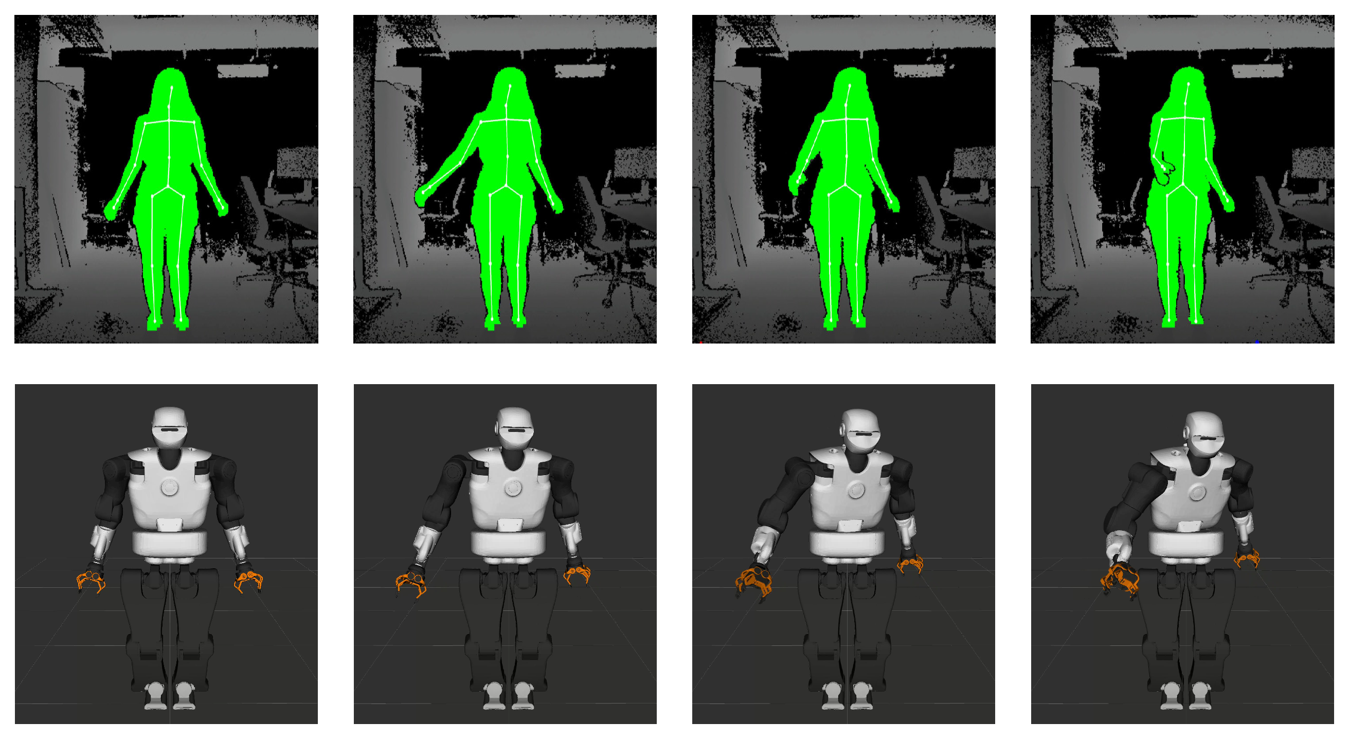
2.1. Kinematic Motion Mapping

We use 3D vision and a human body tracker to capture human movements in real time. The first step in the proposed approach is to map the observed human motion onto the humanoid robot’s kinematic structure. The processing of the captured data involves resolving issues such as the correspondence problem and managing noisy sensory data. The captured movements may exceed the robot’s joint limits, potentially harming the robot if the motion is transferred unaltered.

Our mapping method comprises two key components. Firstly, the joint angle motion of a target humanoid robot is derived from the measurements computed by the body tracker. Secondly, the resulting joint angle trajectories are passed through a safety check function that prevent the execution of motions that violate the robot’s joint angle limits. In addition, motions that exceed the velocity limits are slowed down. This ensures that the transferred motion is safe for the execution by the humanoid robot.

Human body trackers generate a stream of positions and orientations of the observed body segments of a human demonstrator. These measurements should be mapped to humanoid robot joint angles. This is achieved by computing the relative orientation of two consecutive body segments with respect to each other. For example, consider the calculation of the joint angles for the humanoid robot shoulder at each measurement time. We start by computing the relative orientation between the body’s trunk and the upper arm segment. The corresponding robot joint angles are then calculated using the combination of Euler angles that matches the kinematics of the target humanoid robot’s shoulder. Once the joint angles are calculated, we apply a linear Kalman filter to smooth the computed joint angle trajectories.

The safety check function first moderates the speed of movement by limiting the velocities that exceed a predefined threshold. This way we prevent fast movements that can be dangerous for the robot. In addition, once any given joint angle approaches the corresponding joint angle limit, we gradually decrease the velocity of joint motion, if necessary coming to a full stop when the desired joint angle is very close to the joint limit.

Please refer to [12,14] for more details about our implementation of kinematic motion mapping.

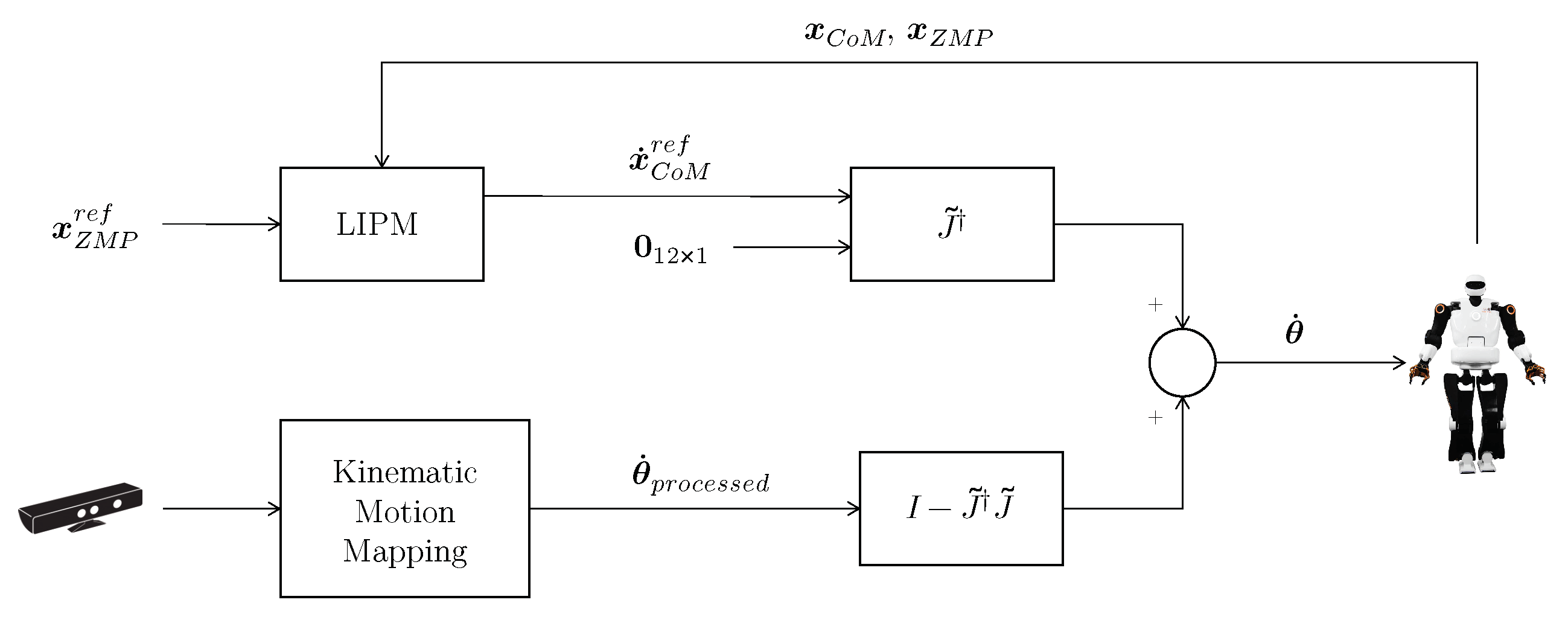
2.2. Stability Control and Motion Mapping

Since we are interested in safe and stable motion imitation, solely mapping the kinematic motion of the human demonstrator to the humanoid robot is insufficient. The directly transferred joint angle trajectories may lead to falls as the robot’s stability is not considered during the motion transfer. To address this issue, we incorporated a stability control mechanism based on the linear inverted pendulum dynamics. This approach accounts for the robot’s mass distribution to ensure the stability of the robot while executing the transferred motions.

The issue of preserving the stability of a humanoid robot is one of the fundamental challenges of humanoid robotics. The most popular stability concept, the zero moment point (ZMP), was introduced by Vukobratović [27] and has been foundational in developing various stability control methods ever since. The ZMP represents an important physical characteristic of a humanoid robot, denoting the point on the ground where the sum of all the moments of the active forces equals zero. The stability criterion derived from the ZMP states that the robot is balanced if its ZMP falls within the convex hull defined by the soles of its feet.

The humanoid robot’s motion space is highly complex and multi-dimensional, making its dynamics nonlinear. To address this complexity, researchers often approximate the robot’s dynamics using point mass models. The linear inverted pendulum model (LIPM) dynamics are widely used, assuming that the entire robot mass is concentrated at its center of mass (CoM) [28,29,30]. Although simplified, this model has proven valuable for stabilization and gait control in humanoid robots [31,32,33,34,35]. By employing the LIPM, the idea is to exploit the dynamic relationship between the robot’s CoM and the ZMP to generate whole-body motion while ensuring that ZMP stays within the support polygon [33]. Considering the dynamics of the LIPM where the whole mass is concentrated at ${\mathit{x}}_{CoM}$, the following relation between the CoM and ZMP can be obtained

$${\ddot{x}}_{CoM}=\omega (x_{CoM}-x_{ZMP}),$$

(1)

$${\ddot{y}}_{CoM}=\omega (y_{CoM}-y_{ZMP}).$$

(2)

Assuming the constant height of the point mass $z_c$, we can compute $\omega =\sqrt{g/z_c}$, the natural frequency of the linear inverted pendulum, where g is the gravity constant. Here, the z axis is assumed to be parallel to the direction of gravity. Alternatively, instead of assuming constant height for the center of mass, the z component of the CoM dynamics can be controlled by defining the natural frequency as ${\displaystyle \omega =\sqrt{\frac{{\ddot{z}}_{CoM}+g}{z_{CoM}-z_{ZMP}}}}$. In essence, this approach closely resembles the dynamics of the linear inverted pendulum, allowing for effective ZMP control by controlling the center of mass motion.

Based on the relationship between the center of mass and the ZMP given by Equations (1) and (2), Sugihara et al. [33] showed that using any control method for the inverted pendulum control, a reference ZMP can be maintained within the support polygon by controlling the CoM. By employing a simple P-controller, the reference ZMP velocity can be calculated so that the measured ZMP is being pushed toward the center of the support polygon, ${\mathit{x}}_{CSP}=[x_{CSP},y_{CSP}]$, as

$$\begin{array}{ccc}\hfill {\dot{x}}_{ZMP}^{ref}& =& \gamma (x_{CSP}-x_{ZMP}),\hfill \end{array}$$

(3)

$$\begin{array}{ccc}\hfill {\dot{y}}_{ZMP}^{ref}& =& \gamma (y_{CSP}-y_{ZMP}),\hfill \end{array}$$

(4)

where $\gamma$ is a positive gain. Equations (3) and (4) are integrated to obtain the new reference ZMP. Then, using the equations of motion (1) and (2), referential dynamics for the horizontal part of the center of mass can be calculated using the referential ZMP as

$$\begin{array}{ccc}\hfill {\ddot{x}}_{CoM}^{ref}& =& \omega (x_{CoM}-x_{ZMP}^{ref}),\hfill \end{array}$$

(5)

$$\begin{array}{ccc}\hfill {\ddot{y}}_{CoM}^{ref}& =& \omega (y_{CoM}-y_{ZMP}^{ref}).\hfill \end{array}$$

(6)

The desired dynamics of the center of mass can be attained by integrating the Equations (5) and (6). The relationship between the motion of the center of mass and the robot’s joint angles is given by the Jacobian of the center of mass ${\mathit{J}}_{CoM}$, which relates the joint velocities to the velocity of the center of mass as

$${\dot{\mathit{x}}}_{CoM}={\mathit{J}}_{CoM}\dot{\theta }.$$

(7)

The Jacobian of the center of mass ${\mathit{J}}_{CoM}\in {\mathbb{R}}^{3\times n}$, with n being the number of degrees of freedom, is defined as follows:

$${\mathit{J}}_{CoM}=\frac{\partial {\mathit{x}}_{CoM}}{\partial \theta }.$$

(8)

Using (7), a stable whole body motion of a humanoid robot can be generated by following the desired stabilized trajectory of the center of mass.

Considering that the humanoid robot has no fixed base frame, it becomes crucial to take into account the floating point dynamics and apply additional constraints to keep the robot stable. Sugihara et al. [33] discussed how to apply constraints both in joint and in Cartesian space. We are interested in generating whole-body motion while ensuring contact with the ground on both feet of the robot. Thus, it makes sense to constrain the poses of both feet to remain stationary and maintain contact with the ground. These constraints are expressed as follows:

$$\mathbf{0}=\left[\begin{array}{c}{\dot{\mathit{x}}}_{LF}\\ {\omega }_{LF}\end{array}\right]={\mathit{J}}_{LF}\dot{\theta },$$

(9)

$$\mathbf{0}=\left[\begin{array}{c}{\dot{\mathit{x}}}_{RF}\\ {\omega }_{RF}\end{array}\right]={\mathit{J}}_{RF}\dot{\theta },$$

(10)

where ${\dot{\mathit{x}}}_{LF}$ and ${\omega }_{LF}$ are the linear and angular velocity of the left foot, while ${\dot{\mathit{x}}}_{RF}$ and ${\omega }_{RF}$ denote the linear and angular velocity of the right foot. ${\mathit{J}}_{LF}$ and ${\mathit{J}}_{RF}\in {\mathbb{R}}^{6\times n}$, expressed in the fixed world coordinate system, are the left and right foot Jacobians, respectively. They establish the relationship between the joint velocities and the linear and angular velocities of the feet.

Finally, by combining the stable desired trajectory of the robot’s center of mass and the constant pose of the robot’s feet, we can generate joint velocities of stable motion using the following relationship:

$$\left[\begin{array}{c}{\dot{\mathit{x}}}_{CoM}\\ \mathbf{0}\\ \mathbf{0}\end{array}\right]=\tilde{\mathit{J}}\dot{\theta },\tilde{\mathit{J}}=\left[\begin{array}{c}{\mathit{J}}_{CoM}\\ {\mathit{J}}_{LF}\\ {\mathit{J}}_{RF}\end{array}\right].$$

(11)

Using Equation (11) and the desired velocity of the center of mass calculated by integrating Equations (5) and (6), we compute the joint velocities that preserve the stability of the robot

$$\dot{\theta }={\tilde{\mathit{J}}}^{†}\left[\begin{array}{c}{\dot{\mathit{x}}}_{CoM}\\ \mathbf{0}\\ \mathbf{0}\end{array}\right],$$

(12)

where ${\tilde{\mathit{J}}}^{†}$ is the Moore–Penrose pseudoinverse of $\tilde{\mathit{J}}$. Furthermore, the redundancy of the humanoid robot allows for an implementation of multi-task inverse kinematics alongside the stability control. Thus, we can implement stable motion imitation by solving two tasks, of which the primary task is stability control and the secondary task is motion imitation executed in the null space of the primary task. This results in the following control strategy:

$$\dot{\theta }={\tilde{\mathit{J}}}^{†}\left[\begin{array}{c}{\dot{\mathit{x}}}_{CoM}\\ \mathbf{0}\\ \mathbf{0}\end{array}\right]+\mathit{N}{\dot{\theta }}_{\mathrm{processed}},$$

(13)

where $\mathit{N}=(\mathit{I}-{\tilde{\mathit{J}}}^{†}\tilde{\mathit{J}})$ is the null space projection matrix of $\tilde{\mathit{J}}$ and ${\dot{\theta }}_{\mathrm{processed}}$ are the joint velocities acquired from the demonstrated motion and processed with the safety modules. Figure 1 shows the process of obtaining a stable reproduction of human demonstrations.

Utilizing Equation (13), we can generate stable joint trajectories demonstrated by a human. We use each generated stable motion trajectory to initialize the reinforcement learning process, which adapts the motion to meet specific task requirements. Figure 2 shows a sequence of snapshots showing the demonstrated reaching motion to a point in space, along with the corresponding reproduced motion by the robot, altered to preserve the robot’s stability.

3. Motion Adaptation by Reinforcement Learning

The process of stable motion imitation effectively addresses both the kinematics and dynamics of the robot. However, this results in a modified reproduction of the initially demonstrated trajectory. The extracted joint angle motion thus results in a suboptimal control policy for tasks requiring high precision, such as reaching. Thus, the transferred motion needs to be adapted to fulfill the task requirements. This can be achieved by RL algorithms, where the imitated human motion serves as an initial control policy. The aim of the RL is to enhance this initial policy, taking into consideration the specific task requirements and physical constraints of the robot.

As mentioned before, when applying RL to complex robotic systems like humanoid robots, the problem known as the “curse of dimensionality” poses a significant challenge. Despite RL algorithms’ ability to create new control policies, the curse of dimensionality is still an ongoing research concern and often prevents fast and reliable learning. As was shown in [16], the PI² algorithm is able to handle the complexity of a humanoid robot while also providing fast convergence. This approach stands out when measuring the algorithm performance and speed of convergence when compared to gradient-based RL algorithms such as REINFORCE [23] and Natural-Actor-Critic [22].

The Policy Improvement with Path integrals is a probabilistic reinforcement learning algorithm derived from the principles of stochastic optimal control and path integrals. The algorithm uses probability-weighted averaging to perform a parameter update instead of using an estimate of the gradient, as is the case with many RL algorithms. PI² requires minimal tuning of the parameters with the exploration noise being the only tunable parameter. However, the modification used in this work involves a method that is able to automatically determine the exploration magnitude, as proposed by Stulp et al. [19]. The modified method, called PI²-CMA incorporates a covariance matrix adaptation based on [25,26], which enables automatic adaptation of the exploration matrix [36]. Consequently, the robot should be able to determine the trade-off between exploration and exploitation autonomously.

The PI²-CMA learns a parameterized policy. Using a parameterized policy, the curse of dimensionality is avoided and the algorithm optimizes a relatively small number of parameters representing the parameterized task trajectories. In this study, we utilize Dynamical Movement Primitives (DMPs) [37,38], a widely used method for representing robot trajectories. The DMP encoding is utilized to parameterize the reproduced human demonstrations resulting from the stable motion imitation system, generating an initial trajectory that is subsequently improved by the RL process. The trajectory parameterization is a crucial step when learning a task trajectory. The DMP parameterization offers several advantages: it represents the motion with a small number of parameters, reduces the impact of noise present in demonstrations, and generates smooth motion trajectories. The DMP formulation is based on a stable dynamical system and, therefore, ensures stable dynamics of the encoded trajectories. Another advantage is that the learned trajectory can be easily adapted to different goals without modifying its underlying shape. Additionally, this representation proves resilient to external disturbances, further enhancing the robustness of the learned motion trajectories.

3.1. Cost Function

The performance of PI² algorithm depends on the selected cost function. One of the crucial challenges in reinforcement learning is the design of the cost function with respect to which the robot motion is optimized. The cost object function typically defines the goal and shapes the robot behavior with respect to the requirements of the task. We designed a cost function that addresses the requirements of the reaching behavior

$$C\left(\mathsf{\tau }\right)=w_{stab}{C}_{stab}\left(\mathsf{\tau }\right)+w_{pos}{C}_{pos}\left(\mathsf{\tau }\right)+w_{ori}{C}_{ori}\left(\mathsf{\tau }\right)+w_{traj}{C}_{traj}\left(\mathsf{\tau }\right)+w_{acc}{C}_{acc}\left(\mathsf{\tau }\right).$$

(14)

The overall cost function is a weighted sum of objective functions that, respectively, address the stability of the robot ($C_{stab}$), accuracy of reaching motion in terms of final position and orientation ($C_{pos},C_{ori}$), the similarity to the initial demonstration ($C_{traj}$), and the smoothness of the reaching motion ($C_{acc}$). Our focus is on independently assessing the effect of the cost function weights, and as such, we assign a distinct weight to each individual cost term. Having explicit weights for each term allows us to conduct separate analysis of their respective contributions. It is worth noting that while the absolute scaling of the cost function weights does not affect the optimal solution, maintaining their relative scaling is crucial. The cost function terms in Equation (14) are defined as follows:

$$\begin{array}{ccc}\hfill C_{stab}\left(\mathsf{\tau }\right)& =& \frac{1}{N+1}\sum _{i=0}^N{f}_{stab}\left({\mathit{x}}_{ZMP}\left(t_i\right)\right),\hfill \end{array}$$

(15)

$$\begin{array}{ccc}\hfill C_{pos}\left(\mathsf{\tau }\right)& =& \left|\right|{\mathit{x}}_{ee}\left(T\right)-\mathit{g}\left)\right||,\hfill \end{array}$$

(16)

$$\begin{array}{ccc}\hfill C_{ori}\left(\mathsf{\tau }\right)& =& 2\left|\right|log(\mathit{q}\left(T\right)\ast {\tilde{\mathit{q}}}_g)\left|\right|,\hfill \end{array}$$

(17)

$$\begin{array}{ccc}\hfill C_{traj}\left(\mathsf{\tau }\right)& =& \frac{1}{N+1}\mathrm{DTW}(\mathsf{\tau },{\mathsf{\tau }}_{demonstrated}),\hfill \end{array}$$

(18)

$$\begin{array}{ccc}\hfill C_{acc}\left(\mathsf{\tau }\right)& =& \frac{1}{N+1}\sum _{i=0}^N\left|\right|\ddot{\mathsf{\tau }}\left(t_i\right){\left|\right|}^2,\hfill \end{array}$$

(19)

where

$$f_{stab}\left(\mathit{x}\right)=\left\{\begin{array}{cc}{\left({\displaystyle \frac{{\mathrm{dist}}_{SP}\left({\mathit{x}}_{CSP}\right)}{{\mathrm{dist}}_{SP}\left(\mathit{x}\right)}-1}\right)}^2,\hfill & \mathrm{for}\mathit{x}\in \mathrm{Support}\mathrm{Polygon}\hfill \\ \hfill & \mathrm{and}{\mathrm{dist}}_{SP}\left(\mathit{x}\right)\ge \epsilon >0,\hfill \\ {\left({\displaystyle \frac{{\mathrm{dist}}_{SP}\left({\mathit{x}}_{CSP}\right)}{ϵ}-1}\right)}^2,\hfill & \mathrm{otherwise}.\hfill \end{array}\right.$$

(20)

Here, ${\mathrm{dist}}_{SP}$ denotes the function that computes the Euclidean distance of the point $\mathit{x}$ from the border of the support polygon and ${\mathit{x}}_{CSP}$ is the constant center of the support polygon, i.e., the point within the support polygon that is the furthest away from the boundary. Note that

$$0\le {\left(\frac{{\mathrm{dist}}_{SP}\left({\mathit{x}}_{CSP}\right)}{{\mathrm{dist}}_{SP}\left(\mathit{x}\right)}-1\right)}^2<\infty ,\forall \mathit{x}\in \mathrm{Support}\mathrm{Polygon}.$$

(21)

The cost function (21) is equal to zero if $\mathit{x}$ coincides with the center of the support polygon and tends towards infinity as the ZMP approaches the border of the suppport polygon. However, we defined $f_{stab}\left(\mathit{x}\right)$ so that the cost function is bounded when $\mathit{x}$ approaches the $\epsilon$-boundary of the support polygon or when the measured $\mathit{x}$ is outside of the support polygon. We further assume that the feet are stationary and fixed to the ground.

The goal position cost function (16) calculates the Euclidean distance between the robot’s end-effector position and the desired position at the end of the reaching motion. Here, T is the final time step of the current rollout. The goal orientation cost function (17) uses the logarithmic map to calculate the distance metric on ${\mathrm{S}}^3$ between the two orientations represented by the quaternions of the desired orientation and the orientation of the end-effector at the end of the trajectory [39]. The trajectory similarity cost (18) is calculated as the dynamic time warping distance between the performed trajectory and the initially demonstrated trajectory. Additionally, we added a smoothing term (19) that minimizes the joint accelerations arising during the execution of each rollout.

The designed cost function yields a single value about the performance of the executed trajectory, eliminating the temporal averaging step implemented in PI²-CMA. Consequently, the exploration of the parameter vector remains constant during the rollout execution. Therefore, as explained in [40], the problem can be defined also as a black-box optimization problem. In [40], the authors propose a simplification of the PI² algorithm that transforms it to a black-box optimization method, referred to as PI^BB. The PI^BB algorithm lacks the covariance matrix adaptation process. In our case, however, the exploration is still varied and adapted throughout the learning using the covariance matrix adaptation method. We implement this learning process using the DmpBbo library [41].

4. Analysis of Influence of Different Cost Function Terms on the Learnt Motions

In this section, we present an experimental analysis of the effects of different cost function terms on the final reaching motion obtained by reinforcement learning. Our analysis includes a sensitivity study exploring the overall task performance under different weight configurations. The evaluation begins with a foundational cost function comprising reaching accuracy terms and systematically introduces additional cost function terms to observe their respective impacts. The learning approach described in Section 2 and Section 3 is shown in Figure 3.

4.1. Experimental Setting

In our experiments, we focused on the learning of reaching movements on a humanoid robot TALOS [42], initially obtained from a human demonstration, as explained in Section 2.1. The initial demonstration represents a reaching motion for the right end-effector, i.e., the robot’s right wrist, as shown in Figure 2. The final reaching position was within the robot’s upper body reachable workspace, as shown in Figure 4. Therefore, out of TALOS’ 32 degrees of freedom, the learning process was conducted on 18, i.e., those associated with the upper body joints. The lower body joints were fixed, maintaining their initial values. For the representation of joint trajectories, we employed the DMP methodology as outlined in [38]. Each joint trajectory is encoded with a DMP, which contains 20 parameters (weights) to shape the demonstrated trajectory. These parameters are initially computed from our stabilized user demonstration. To fully specify a DMP, we need an additional parameter specifying the final desired joint configuration. As a result, the parameter vector for the reinforcement learning procedure introduced in Section 3 comprises 360 values of weights (for 18 degrees of freedom), alongside additional 18 values specifying the final joint configuration (goal) on the trajectory. This brings the total number of parameters for the RL algorithm to determine to 378.

The motion refinement process was conducted in the Gazebo simulation environment of TALOS. The initial stable motion was optimized by the PI²-CMA method using a cost function (14). All learning sessions were performed with 150 updates, using 30 reaching motion rollouts per update. For the exploration strategy, we chose higher initial exploration values for the robot’s arm joints and lower values for the head and torso joints. However, the PI²-CMA algorithm should be able to automatically determine the optimal covariance matrix within the learning process. By experimenting with different combinations of weights in cost function (14), we analyzed the effect of different cost terms on the final (optimal) reaching trajectory.

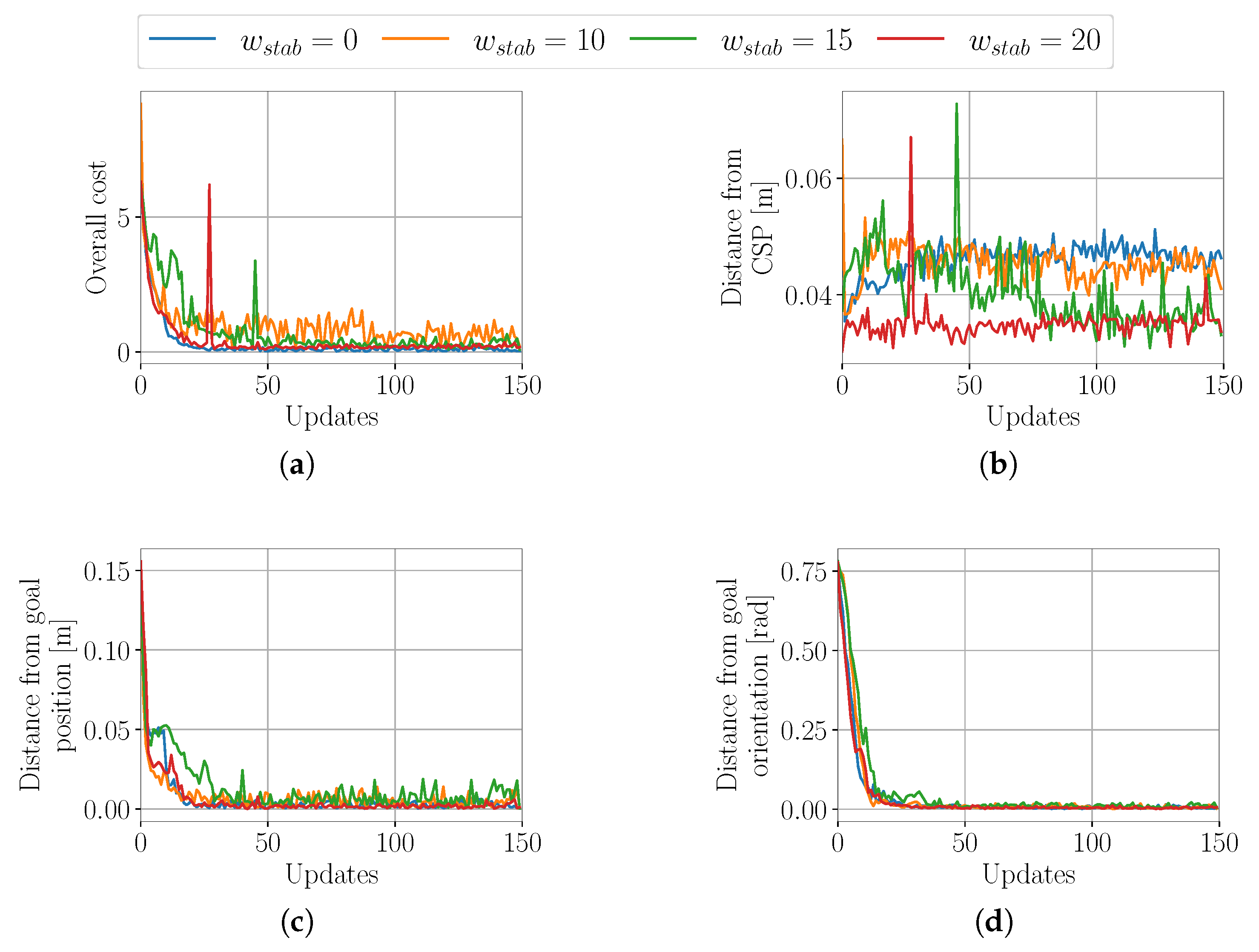
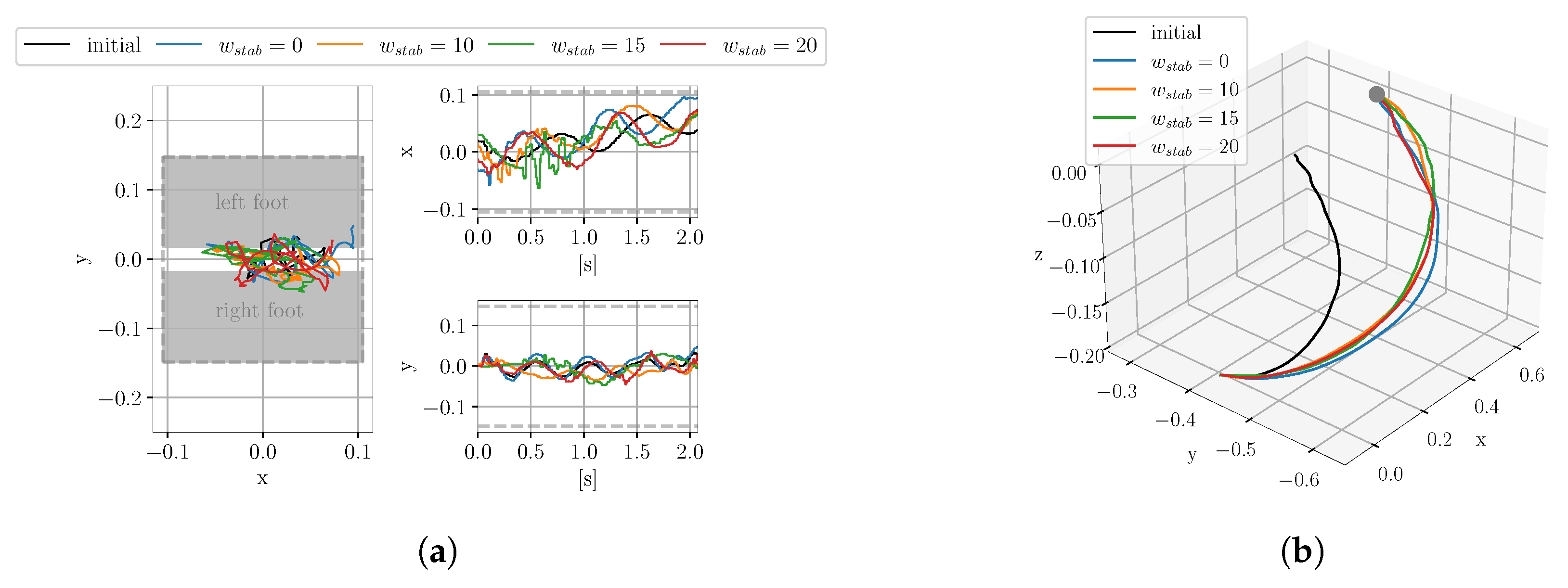
4.1.1. Evaluation of the Influence of the Stability Cost

We started our analysis by setting only the weights of the cost terms addressing the stability and reaching accuracy in cost function (14) to non-zero values. The weights of the trajectory similarity term as well as the smoothing term were thus set to zero. The weights associated with position and orientation cost terms were set to $w_{pos}=20$ and $w_{ori}=4$, respectively. As discussed in Section 3.1, it is essential to maintain the proper relative scaling between these weights. In this context, the choice of $w_{pos}=20$ and $w_{ori}=4$ is made based on a 5:1 ratio between the position and orientation costs observed during the initial demonstration. This ensures that both position and orientation have a similar influence on the overall cost function, contributing to balanced convergence between these two terms. To evaluate the effect of different stability weights, we performed the RL process with 4 different $w_{stab}$, i.e., $w_{stab}=0,10,15,20,$ aiming to provide a comparable scaling as the final position and orientation weights. Although learning always starts with an initially stable motion (acquired by the motion mapping approach described in Section 2.2), the robot could become unstable due to the exploration process. The aim of RL is to maintain and possibly improve the stability of the robot as well as other task requirements.

The results coming from RL sessions with four different stability weights are displayed in Figure 5. The learning curves in Figure 5a show convergence after approximately 30 updates in all 4 cases. Good reaching accuracy was achieved by all four weights, as plotted in Figure 5c,d. The main difference is visible in the stability term. Figure 5b depicts the average distance of the measured center of pressure to the center of the support polygon throughout the learning process. As expected, the higher stability weight contributes to the improved stability of the robot.

Good task performance is evident also from the trajectory of the ZMP and the 3D spatial path of the end-effector, respectively, as shown in Figure 6a,b. The robot maintains the ZMP within the support polygon for each configuration of weights. As expected, the learning session with the highest stability weight shows the most stable motion of the ZMP. Figure 6b provides insight into the evolution of the end-effector trajectory. Despite the lack of the trajectory similarity term in the cost function, the end-effector learns to accurately reach the desired pose while preserving the initially demonstrated trajectory shape.

Table 1. Statistical analysis of reaching accuracy and stability of the robot when using different stability cost weights to optimize the reaching motion. The weights of the other cost terms were set as follows: $w_{pos}=20,w_{ori}=4,w_{traj}=0.0,w_{acc}=0.0$.

	Position [m]		Orientation [rad]		Distance from CSP [m]
	Avg	Min	Avg	Min	Avg	Min
$w_{stab}=0$	0.0031	0.0003	0.0059	0.0015	0.0469	0.0440
$w_{stab}=10$	0.0069	0.0011	0.0152	0.0039	0.0494	0.0426
$w_{stab}=15$	0.0079	0.0003	0.0103	0.0015	0.0364	0.0308
$w_{stab}=20$	0.0020	0.0003	0.0047	0.0008	0.0352	0.0302

provides the statistical analysis of reaching accuracy and stability of the robot when using different stability cost weights to optimize the reaching motion. The table presents the average and minimal errors for position and orientation observed in the last 50 updates as well as the average and the minimal distance between the measured center of pressure and the center of the support polygon in the last 50 updates. All weight configurations demonstrate a reaching accuracy with low positional and orientational errors. As the highest stability weight $w_{stab}=20$ only negligibly influences the accuracy of reaching, we used this value in the rest of our analysis.

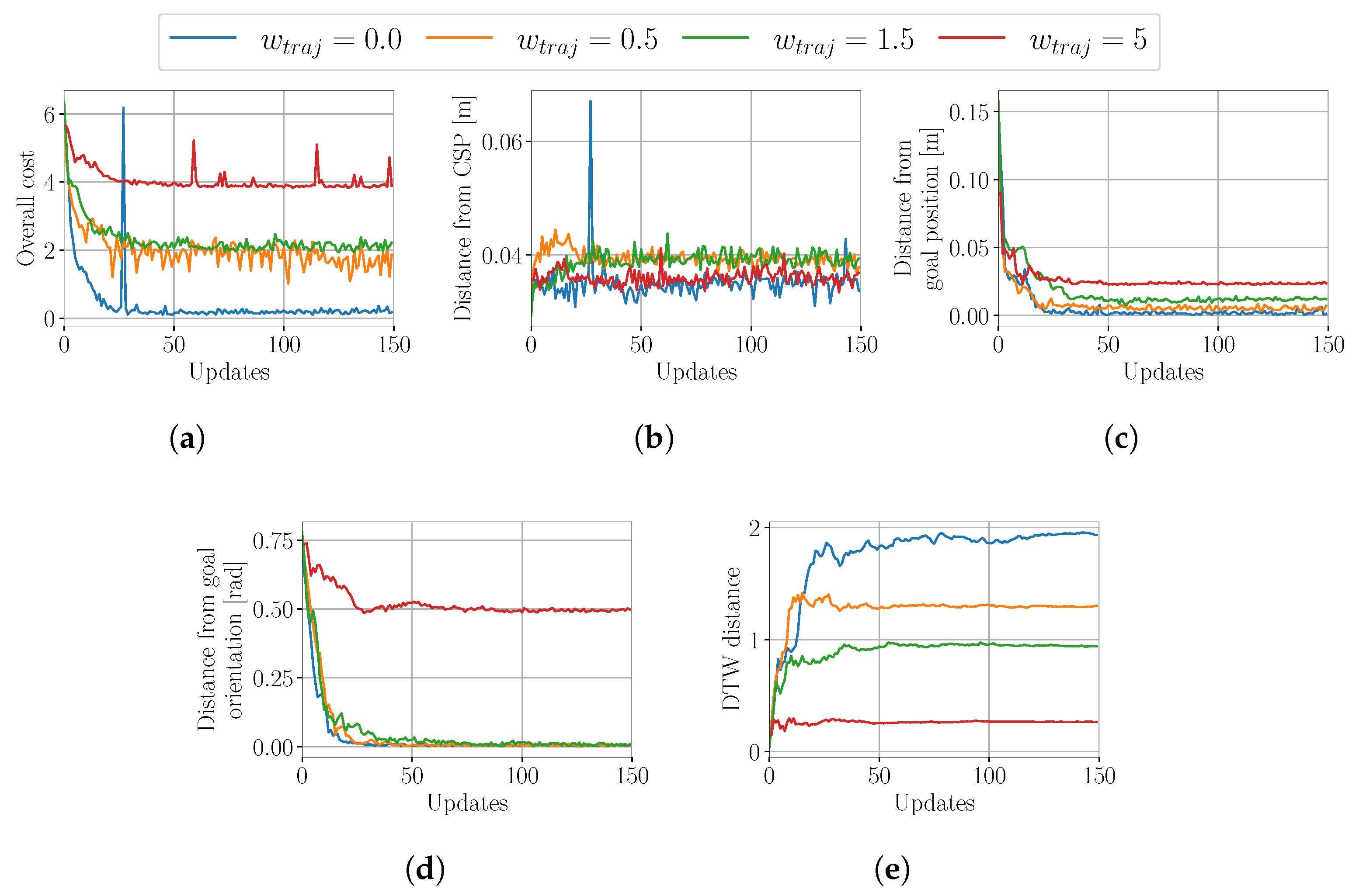
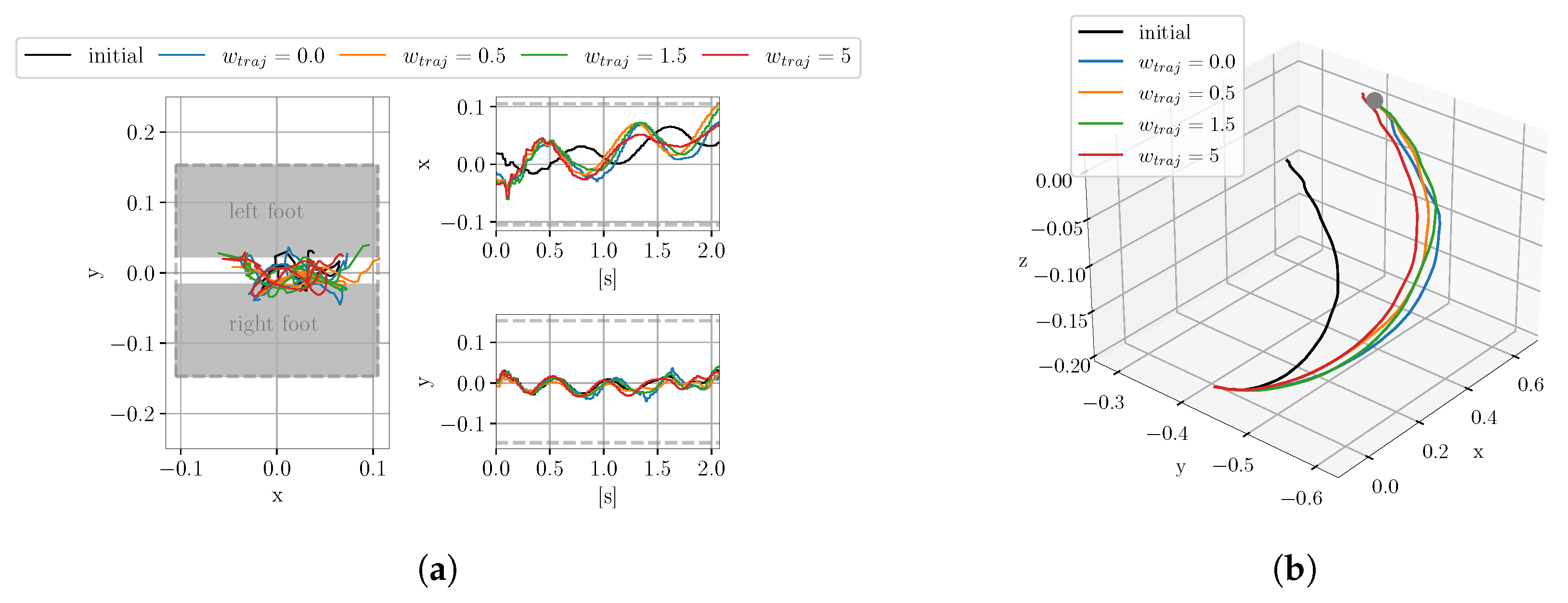
4.1.2. Evaluation of the Influence of the Trajectory Similarity Cost

Next, we analyzed the impact of the trajectory similarity term. As justified in Section 4.1.1, the weight for the stability was chosen to be $w_{stab}=20$. The weights associated with the accuracy of reaching position and orientation cost were kept at $w_{pos}=20$ and $w_{ori}=4$, respectively, while the weight of the smoothing term was set to 0. We analyzed the learning processes by varying the trajectory similarity cost weight, where we selected $w_{traj}=0.0,0.5,1.5,5$, aiming to provide similar or higher scaling than the other cost terms. Learning curves for the different weight configurations are shown in Figure 7a. As expected, the highest trajectory similarity weight yields the smallest deviation from the initial trajectory. However, this comes at the expense of the compromised reaching accuracy as the weight increases. We observe a consistent pattern of the reduced reaching accuracy as the trajectory similarity weight increases.

The performance of different trajectory similarity weights in terms of stability are visualized through the ZMP trajectories in Figure 8a. It turns out that the trajectory similarity term did not significantly influence the stability of the robot. Finally, in Figure 8b we observe that the spatial course of all of the computed reaching motions is similar to the spatial course of the initial reaching trajectory. Due to the generalization properties inherent in the DMP representation, even the trajectory computed with $w_{traj}=0$ approximates the overall spatial course of the resulting reaching motion well.

Table 2. Statistical analysis of the reaching accuracy and trajectory similarity when using different trajectory similarity cost weights to optimize the reaching motion. The weights of the other cost terms were set as follows: $w_{pos}=20,w_{ori}=4,w_{stab}=20,w_{acc}=0.0$.

	Position [m]		Orientation [rad]		DTW Distance
	Avg	Min	Avg	Min	Avg	Min
$w_{traj}=0.0$	0.0020	0.0003	0.0047	0.0008	1.9202	1.8585
$w_{traj}=0.5$	0.0053	0.0035	0.0055	0.0003	1.2956	1.2847
$w_{traj}=1.5$	0.0120	0.0102	0.0086	0.0005	0.9465	0.9375
$w_{traj}=5$	0.0234	0.0227	0.4946	0.4868	0.2672	0.2653

provides numerical values for the accuracy of reaching and for trajectory similarity. The table presents the average and minimal errors for position and orientation observed in the last 50 updates. Furthermore, the average and minimal DTW distance between the initial reaching motion and the computed reaching motions in the last 50 updates are also provided. The results presented in Table 2 confirm the negative impact of the trajectory similarity term on the reaching accuracy. While the optimal trajectory from the learning session with the highest weight ($w_{traj}=5$) is the closest to the initially demonstrated trajectory, the reaching accuracy is compromised and the robot fails to reach the desired pose. Given that the results in Figure 8a and Table 2 demonstrate that the trajectory similarity weight only negligibly improves the trajectory shape and that the initial trajectory shape is well preserved even when $w_{traj}=0$, we conclude that the best choice for the weight of the trajectory cost term is $w_{traj}=0$.

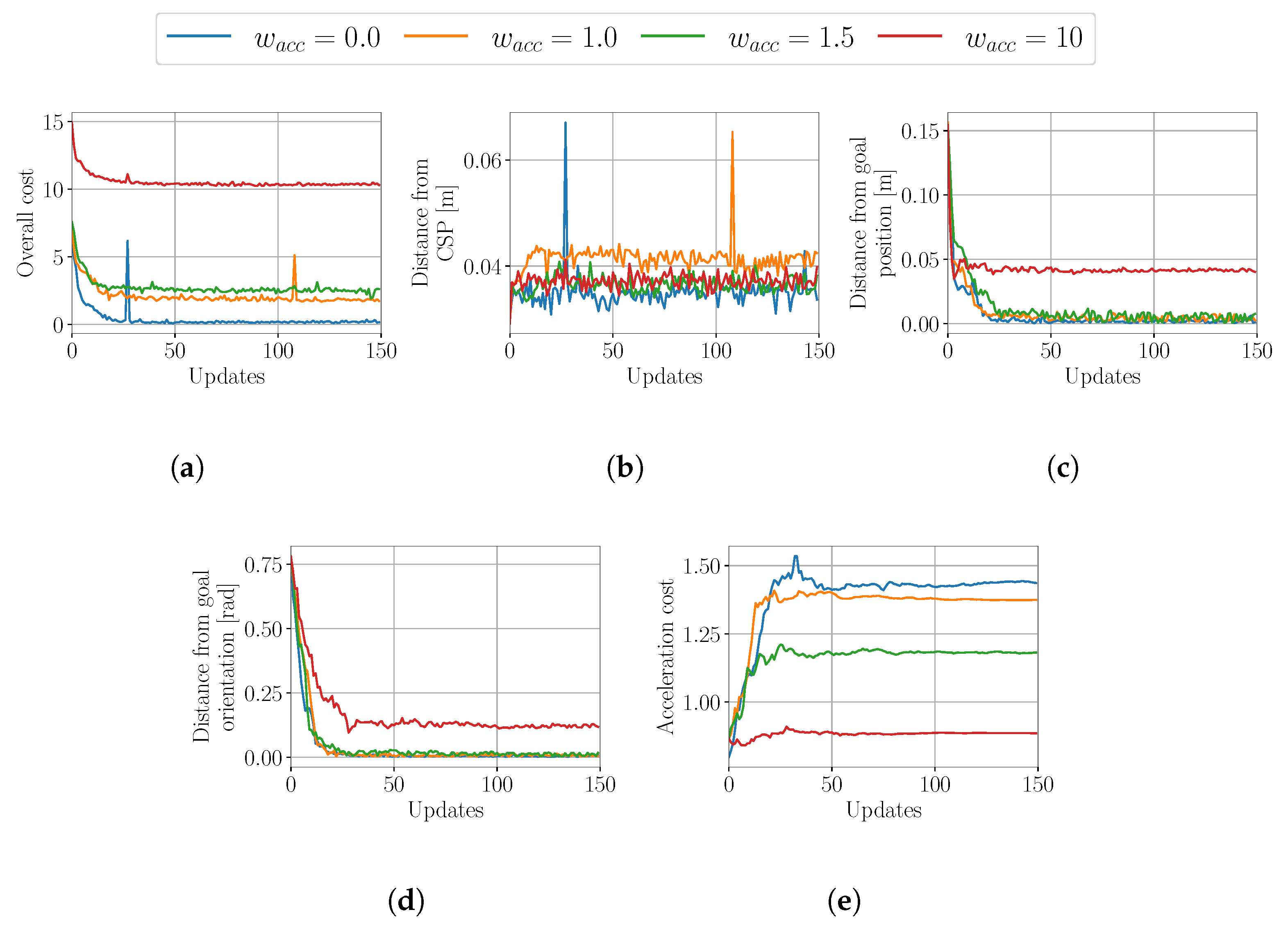
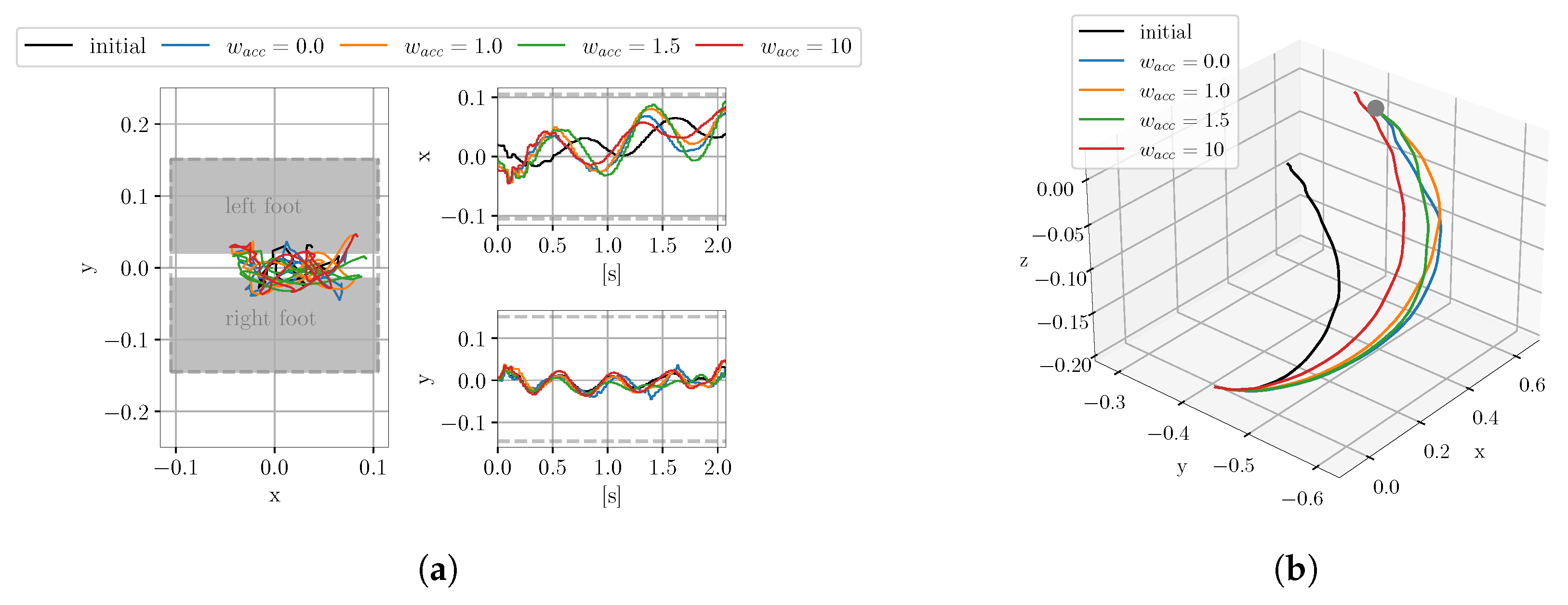
4.1.3. Evaluation of the Influence of the Smoothing Cost

Finally, we also investigated the impact of the smoothing term in cost function (14). Its purpose is to ensure the generation of smooth joint trajectories. Based on the results of Section 4.1.1 and Section 4.1.2, we set $w_{pos}=20$, $w_{ori}=4$, $w_{stab}=20$, and $w_{traj}=0.0$. In Figure 9, we compare the performance of learning when varying acceleration cost weight, specifically $w_{acc}=0.0,1.0,1.5,10$, which will provide comparable but also higher scaling than the other cost terms included in the learning process. As evident from Figure 9e, the configuration with the highest smoothness weight results in the lowest cost for acceleration.

The resulting ZMP trajectories and end-effector paths are depicted in Figure 10a,b, respectively. Note that the configuration with the highest acceleration weight compromises the reaching accuracy and also alters the shape of the reaching trajectory.

Table 3. Statistical analysis of the reaching accuracy and smoothing cost when using different smoothing cost weights to optimize the reaching motion. The weights of the other cost terms were set as follows: $w_{pos}=20,w_{ori}=4,w_{stab}=20,w_{traj}=0.0$.

	Position [m]		Orientation [rad]		Smoothing Cost
	Avg	Min	Avg	Min	Avg	Min
$w_{acc}=0.0$	0.0020	0.0003	0.0047	0.0008	1.4340	1.4215
$w_{acc}=1.0$	0.0041	0.0015	0.0077	0.0024	1.3749	1.3733
$w_{acc}=1.5$	0.0047	0.0005	0.0109	0.0021	1.1814	1.1779
$w_{acc}=10$	0.0414	0.0402	0.1195	0.1114	0.8862	0.8851

provides the statistical analysis of the reaching accuracy and smoothing cost when evaluating different smoothing cost weights when learning the reaching motion. Average and minimal positional and orientational errors are presented as well as the average and minimal smoothing cost between the initial reaching motion and the computed reaching motions in the last 50 updates. The statistical analysis in Table 3 makes the trend of increased deviation from the desired final reaching pose as the smoothness weight increases clear. However, the configuration with a smoothness weight of $w_{acc}=1.0$ maintains good reaching accuracy while achieving a smoother reaching trajectory, as evident from Figure 10b. Consequently, we conclude that the weight configurations with $w_{acc}=0.0$ and $w_{acc}=1.0$ both offer good solutions.

4.1.4. Systematic Search for the Optimal Weights of the Stability Cost Term

Based on the findings presented in Section 4.1.2 and Section 4.1.3, the trajectory similarity term and the smoothing term did not enhance the task performance. On the other hand, Section 4.1.1 shows that it is important to consider the stability terms. Thus, the most suitable weight configuration includes the weights for position and orientation reaching errors and the stability cost term. As disucssed in Section 4.1.1, the weights of position and orientation terms in the cost function can be set to preselected constant values. Here, we discuss how to automate the selection of optimal weight for the stability cost term. To do this, we conducted a grid search across stability weights, ranging from 0 to 60 in increments of 5.

In Figure 11, we present the average cost associated with each stability weight from the conducted grid search. Clearly, the relationship between the stability weight and the defined cost function as well as the specific cost terms is non-convex. Having a non-convex relation discards the applicability of most of the traditional optimization techniques, such as bisection and gradient-decent approaches. Therefore, a random search or grid search are the simplest approaches to get a better insight of the parameter impact. For the grid search conducted in this experiment, the weight $w_{stab}$ that results in the minimal overall cost is $w_{stab}=40$.

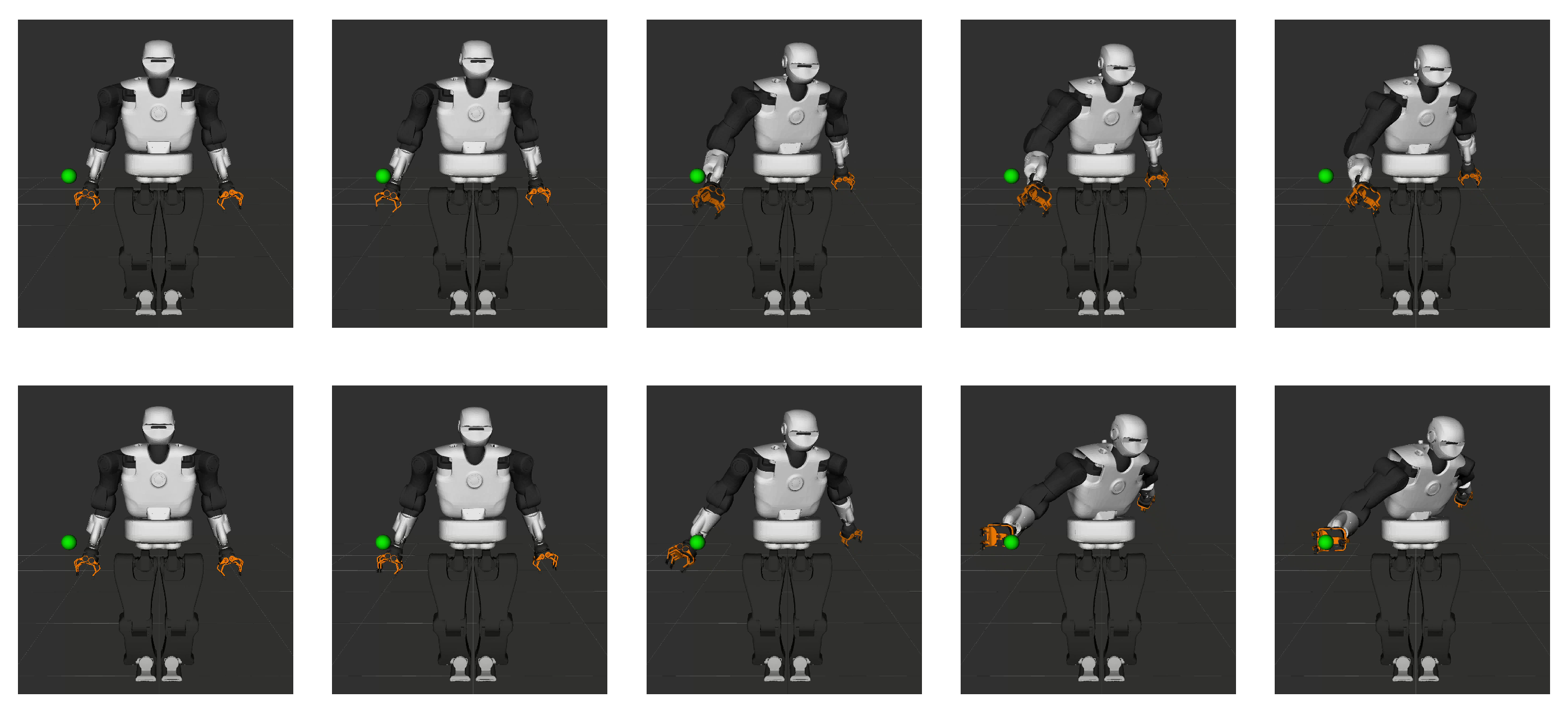
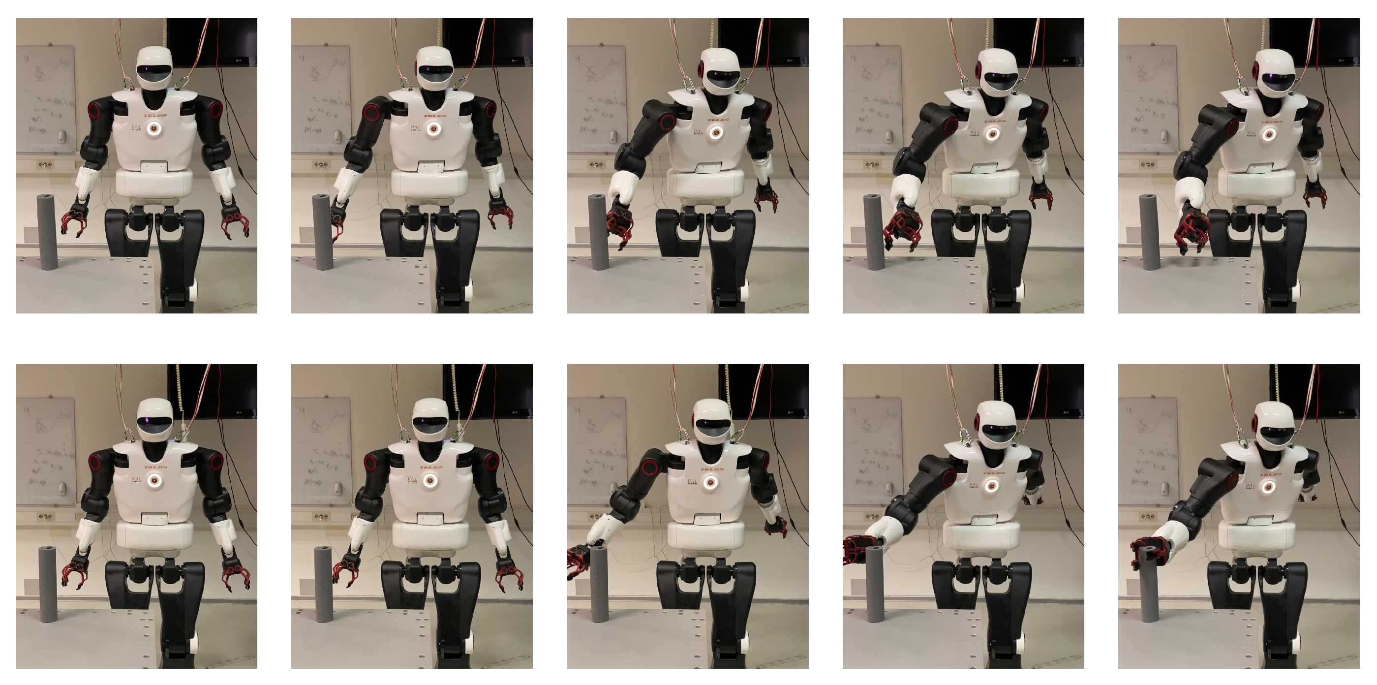
5. Execution of Trajectories Learnt in Simulation on the Real Robot

Since all solutions computed by RL resulted in stable and safe reaching motions (see Section 4.1), it was possible to use them directly to generate the reaching motions on the real robot. For evaluation, we used the solution computed with weights set to $w_{pos}=20$, $w_{ori}=4$, $w_{stab}=20$, $w_{traj}=0.0$, and $w_{acc}=0$.

Figure 12b shows the comparison between the reaching trajectories executed in simulation and on the real robot. Clearly, the reality gap is small and there is not considerable deviation between the two trajectories. Notably, the execution of the computed reaching motion on the real robot resulted in a similarly stable ZMP trajectory, as shown in Figure 12a. Figure 13 and Figure 14 show the task execution, illustrating the performance in both simulation and on the real robot. Sequences of the execution of the initial demonstration and the optimal motion in both scenarios is shown, confirming the efficacy of the proposed learning approach in achieving precise reaching motions.

Low discrepancy between the motions in simulation and on the real robot is probably due to the reaching motion that includes only the upper body joint angles. Additionally, no contacts occurred in our experiments. Considering lower body degrees of freedom and tasks that include contacts with the environment, the solution computed in simulation might need to be adapted to ensure its applicability on the real robot. Such an adaptation process can utilize the motion computed in simulation as an initial approximation for the adaptation on the real robot. This should result in faster learning compared to starting from the human-demonstrated trajectories.

The results showing the reaching accuracy and stability performance are given also in

Table 4. Accuracy of reaching motion and stability performance in simulation and on the real robot. The cost function weights when computing the reaching motion were set to the following values: $w_{stab}=20,w_{pos}=20,w_{ori}=4,w_{traj}=0.0,w_{acc}=0.0$.

Position (m)		Orientation (rad)		Distance from CSP (m)
Simulation	Robot	Simulation	Robot	Simulation	Robot
0.0012	0.0056	0.0061	0.0114	0.0337	0.0441

, where the errors for the final reaching position and orientation of the executions in simulation and on the real robot are presented. Additionally, Table 4 shows the average distance between the measured center of pressure and the center of the support polygon while executing the reaching trajectory. There is an insignificant difference between the performance of the simulated robot and the real robot in terms of reachability. The stability cost shows similar distances from the center of the support polygon in both the simulated and real robot reaching motion. The ZMP trajectories plotted in Figure 12a even exhibit less oscillations when the reaching motion is performed by the real robot.

6. Conclusions

In this study, we combined imitation learning and reinforcement learning to effectively teach a humanoid robot how to perform a reaching task while maintaining its stability. Our approach involves transferring an observed human motion to a humanoid robot, accounting for the stability constraints of humanoid robots. The transferred motion is then refined using reinforcement learning with a suitably selected cost function to consider several specific objectives with respect to the desired task. In our study, the selection of suitable cost function components is grounded in statistical analysis of the influence of different cost function terms on the performance of the reaching behavior. The gained insights helped us determine the most effective weight configuration for the selected cost function, ensuring the best performance across multiple task objectives. Our analysis finally led to the conclusion about the best weight configuration and highlighted the importance of various constraints with respect to the overall task performance.

The proposed algorithm was successfully applied to compute reaching motions for a high degree of freedom humanoid robot. It can learn stable reaching trajectories in less than 30 updates. With the proposed approach, the robot can learn a reaching motion to a desired point in 3D space, based on a single observation of human motion. The optimal reaching motions computed by RL in simulation were transferred and assessed on the real robot, demonstrating a negligible gap between simulation and real world. Nevertheless, to tackle more intricate tasks, it is likely that further adjustments to the transferred motion will be necessary to accommodate the variations in the dynamics between the simulated and the real robot.

The proposed framework offers various possibilities for extension. It can be adapted to include more complex whole-body tasks, integrating additional constraints into the learning process. Addressing these more complex tasks will necessitate the adoption of advanced approaches for determining optimal weights. In this context, an automated curriculum learning approach could be utilized to learn an optimal weight configuration by progressively increasing task complexity. On a smaller scale, the method presented in this work is comparable to curriculum learning. In our case, the analysis of task performance was used, whereas curriculum learning would require specifically designed heuristics to identify the optimal combination of weights.

References

1. Kajita, S.; Hirukawa, H.; Harada, K.; Yokoi, K. Introduction to Humanoid Robotics; Springer Tracts in Advanced Robotics; Springer: Berlin/Heidelberg, Germany, 2014. [Google Scholar]
2. Hua, J.; Zeng, L.; Li, G.; Ju, Z. Learning for a Robot: Deep Reinforcement Learning, Imitation Learning, Transfer Learning. Sensors 2021, 21, 1278. [Google Scholar] [CrossRef] [PubMed]
3. Billard, A.; Calinon, S.; Dillmann, R.; Schaal, S. Robot Programming by Demonstration. In Handbook of Robotics; Siciliano, B., Khatib, O., Eds.; Springer: Berlin/Heidelberg, Germany, 2008; pp. 1371–1394. [Google Scholar]
4. Schaal, S. Learning from Demonstration. In Proceedings of the 9th International Conference on Neural Information Processing Systems, Denver, CO, USA, 3–5 December 1996; pp. 1040–1046. [Google Scholar]
5. Argall, B.D.; Chernova, S.; Veloso, M.; Browning, B. A survey of robot learning from demonstration. Robot. Auton. Syst. 2009, 57, 469–483. [Google Scholar] [CrossRef]
6. Ude, A.; Riley, M.; Atkeson, C.G. Planning of joint trajectories for humanoid robots using B-spline wavelets. In Proceedings of the IEEE International Conference on Robotics and Automation (ICRA), San Francisco, CA, USA, 24–28 April 2000; pp. 2223–2228. [Google Scholar]
7. Ude, A.; Atkeson, C.G.; Riley, M. Programming full-body movements for humanoid robots by observation. Robot. Auton. Syst. 2004, 47, 93–108. [Google Scholar] [CrossRef]
8. Koenemann, J.; Burget, F.; Bennewitz, M. Real-time imitation of human whole-body motions by humanoids. In Proceedings of the IEEE International Conference on Robotics and Automation (ICRA), Hong Kong, China, 31 May–7 June 2014; pp. 2806–2812. [Google Scholar]
9. Zhang, L.; Cheng, Z.; Gan, Y.; Zhu, G.; Shen, P.; Song, J. Fast human whole body motion imitation algorithm for humanoid robots. In Proceedings of the IEEE International Conference on Robotics and Biomimetics (ROBIO), Qingdao, China, 3–7 December 2016; pp. 1430–1435. [Google Scholar]
10. Zhang, Z.; Niu, Y.; Yan, Z.; Lin, S. Real-Time Whole-Body Imitation by Humanoid Robots and Task-Oriented Teleoperation Using an Analytical Mapping Method and Quantitative Evaluation. Appl. Sci. 2018, 8, 2005. [Google Scholar] [CrossRef]
11. Mi, J.; Takahashi, Y. Whole-Body Joint Angle Estimation for Real-Time Humanoid Robot Imitation Based on Gaussian Process Dynamical Model and Particle Filter. Appl. Sci. 2020, 10, 5. [Google Scholar] [CrossRef]
12. Savevska, K.; Simonič, M.; Ude, A. Modular Real-Time System for Upper-Body Motion Imitation on Humanoid Robot Talos. In Advances in Service and Industrial Robotics, RAAD 2021; Zeghloul, S., Laribi, M.A., Sandoval, J., Eds.; Springer: Cham, Switzerland, 2021; pp. 229–239. [Google Scholar]
13. Vuga, R.; Ogrinc, M.; Gams, A.; Petrič, T.; Sugimoto, N.; Ude, A.; Morimoto, J. Motion capture and reinforcement learning of dynamically stable humanoid movement primitives. In Proceedings of the IEEE International Conference on Robotics and Automation (ICRA), Karlsruhe, Germany, 6–10 May 2013; pp. 5284–5290. [Google Scholar]
14. Savevska, K.; Ude, A. Teaching Humanoid Robot Reaching Motion by Imitation and Reinforcement Learning. In Advances in Service and Industrial Robotics, RAAD2023; Petrič, T., Ude, A., Žlajpah, L., Eds.; Springer: Cham, Switzerland, 2023; pp. 53–61. [Google Scholar]
15. Theodorou, E.; Buchli, J.; Schaal, S. Learning Policy Improvements with Path Integrals. J. Mach. Learn. Res. 2010, 9, 828–835. [Google Scholar]
16. Stulp, F.; Buchli, J.; Theodorou, E.; Schaal, S. Reinforcement learning of full-body humanoid motor skills. In Proceedings of the IEEE-RAS International Conference on Humanoid Robots, Nashville, TN, USA, 6–8 December 2010; pp. 405–410. [Google Scholar]
17. Theodorou, E.; Stulp, F.; Buchli, J.; Schaal, S. An Iterative Path Integral Stochastic Optimal Control Approach for Learning Robotic Tasks. IFAC Proc. Vol. 2011, 44, 11594–11601. [Google Scholar] [CrossRef]
18. Theodorou, E.; Buchli, J.; Schaal, S. Reinforcement learning of motor skills in high dimensions: A path integral approach. In Proceedings of the IEEE International Conference on Robotics and Automation (ICRA), Anchorage, AK, USA, 3–7 May 2010; pp. 2397–2403. [Google Scholar]
19. Stulp, F.; Sigaud, O. Path Integral Policy Improvement with Covariance Matrix Adaptation. In Proceedings of the 29th International Conference on Machine Learning (ICML), Edinburgh, UK, 26 June–1 July 2012. [Google Scholar]
20. Fu, J.; Li, C.; Teng, X.; Luo, F.; Li, B. Compound Heuristic Information Guided Policy Improvement for Robot Motor Skill Acquisition. Appl. Sci. 2020, 10, 5346. [Google Scholar] [CrossRef]
21. Kober, J.; Peters, J. Policy search for motor primitives in robotics. Mach. Learn. 2010, 84, 171–203. [Google Scholar] [CrossRef]
22. Peters, J.; Schaal, S. Natural Actor-Critic. Neurocomputing 2008, 71, 1180–1190. [Google Scholar] [CrossRef]
23. Williams, R.J. Simple Statistical Gradient-Following Algorithms for Connectionist Reinforcement Learning. Mach. Learn. 1992, 8, 229–256. [Google Scholar] [CrossRef]
24. Peters, J.; Schaal, S. Policy Gradient Methods for Robotics. In Proceedings of the IEEE/RSJ International Conference on Intelligent Robots and Systems (IROS), Beijing, China, 9–15 October 2006; pp. 2219–2225. [Google Scholar]
25. Mannor, S.; Rubinstein, R.; Gat, Y. The Cross Entropy method for Fast Policy Search. In Proceedings of the Twentieth International Conference on Machine Learning (ICML), Washington, DC, USA, 21–24 August 2003; pp. 512–519. [Google Scholar]
26. Hansen, N.; Ostermeier, A. Completely Derandomized Self-Adaptation in Evolution Strategies. Evol. Comput. 2001, 9, 159–195. [Google Scholar] [CrossRef] [PubMed]
27. Vukobratović, M.; Stepanenko, J. On the stability of anthropomorphic systems. Math. Biosci. 1972, 15, 1–37. [Google Scholar] [CrossRef]
28. Kajita, S.; Tani, K. Study of dynamic biped locomotion on rugged terrain-derivation and application of the linear inverted pendulum mode. In Proceedings of the IEEE International Conference on Robotics and Automation (ICRA), Sacramento, CA, USA, 9–11 April 1991; pp. 1405–1411. [Google Scholar]
29. Kajita, S.; Kanehiro, F.; Kaneko, K.; Yokoi, K.; Hirukawa, H. The 3D linear inverted pendulum mode: A simple modeling for a biped walking pattern generation. In Proceedings of the IEEE/RSJ International Conference on Intelligent Robots and Systems (IROS), Maui, HI, USA, 30 October–3 November 2001; pp. 239–246. [Google Scholar]
30. Yamamoto, K.; Kamioka, T.; Sugihara, T. Survey on model-based biped motion control for humanoid robots. Adv. Robot. 2020, 34, 1353–1369. [Google Scholar] [CrossRef]
31. Kajita, S.; Kanehiro, F.; Kaneko, K.; Fujiwara, K.; Harada, K.; Yokoi, K.; Hirukawa, H. Biped walking pattern generation by using preview control of zero-moment point. In Proceedings of the IEEE International Conference on Robotics and Automation (ICRA), Taipei, Taiwan, 14–19 September 2003; pp. 1620–1626. [Google Scholar]
32. Kajita, S.; Morisawa, M.; Miura, K.; Nakaoka, S.; Harada, K.; Kaneko, K.; Kanehiro, F.; Yokoi, K. Biped walking stabilization based on linear inverted pendulum tracking. In Proceedings of the 2010 IEEE/RSJ International Conference on Intelligent Robots and Systems, Taipei, Taiwan, 18–22 October 2010; pp. 4489–4496. [Google Scholar]
33. Sugihara, T.; Nakamura, Y.; Inoue, H. Real-time humanoid motion generation through ZMP manipulation based on inverted pendulum control. In Proceedings of the IEEE International Conference on Robotics and Automation (ICRA), Washington, DC, USA, 11–15 May 2002; pp. 1404–1409. [Google Scholar]
34. Sugihara, T. Standing stabilizability and stepping maneuver in planar bipedalism based on the best COM-ZMP regulator. In Proceedings of the IEEE International Conference on Robotics and Automation (ICRA), Kobe, Japan, 12–17 May 2009; pp. 1966–1971. [Google Scholar]
35. Sugihara, T.; Morisawa, M. A survey: Dynamics of humanoid robots. Advanced Robotics 2020, 34, 1338–1352. [Google Scholar] [CrossRef]
36. Stulp, F. Adaptive exploration for continual reinforcement learning. In Proceedings of the IEEE/RSJ International Conference on Intelligent Robots and Systems, Vilamoura-Algarve, Portugal, 7–12 October 2012; pp. 1631–1636. [Google Scholar]
37. Ijspeert, A.J.; Nakanishi, J.; Hoffmann, H.; Pastor, P.; Schaal, S. Dynamical Movement Primitives: Learning Attractor Models for Motor Behaviors. Neural Comput. 2013, 25, 328–373. [Google Scholar] [CrossRef]
38. Ude, A.; Gams, A.; Asfour, T.; Morimoto, J. Task-Specific Generalization of Discrete and Periodic Dynamic Movement Primitives. IEEE Trans. Robot. 2010, 26, 800–815. [Google Scholar] [CrossRef]
39. Ude, A. Filtering in a unit quaternion space for model-based object tracking. Robot. Auton. Syst. 1999, 28, 163–172. [Google Scholar] [CrossRef]
40. Stulp, F.; Sigaud, O. Robot Skill Learning: From Reinforcement Learning to Evolution Strategies. Paladyn, J. Behav. Robot. 2013, 4, 49–61. [Google Scholar] [CrossRef]
41. Stulp, F.; Raiola, G. DmpBbo: A versatile Python/C++ library for Function Approximation, Dynamical Movement Primitives, and Black-Box Optimization. J. Open Source Softw. 2019, 4, 1225. [Google Scholar] [CrossRef]
42. Stasse, O.; Flayols, T.; Budhiraja, R.; Giraud-Esclasse, K.; Carpentier, J.; Mirabel, J.; Del Prete, A.; Souéres, P.; Mansard, N.; Lamiraux, F.; et al. TALOS: A new humanoid research platform targeted for industrial applications. In Proceedings of the IEEE-RAS 17th International Conference on Humanoid Robotics (Humanoids), Birmingham, UK, 15–17 November 2017; pp. 689–695. [Google Scholar]
Figure 1. Block diagram of the two-task inverse kinematics process for obtaining stable motion reproduction.
Applsci 14 00039 g001
Figure 2. Sequence of snapshots of the demonstrated and reproduced reaching motion.
Applsci 14 00039 g002
Figure 3. System architecture of the learning process used in this study.
Applsci 14 00039 g003
Figure 4. Visual representation of the experimental setup. The robot needs to learn a reaching motion to the desired point in space represented with the green sphere.
Applsci 14 00039 g004
Figure 5. Learning performance when using different weights for the stability cost term. (a) Cost. (b) Distance from the center of the support polygon. (c) Distance from the desired goal position. (d) Distance from the desired goal orientation.
Applsci 14 00039 g005
Figure 6. Stability of the robot and spatial course of the reaching motions when using different weights for the stability cost term. (a) ZMP trajectories of the initial reaching motion and of the motions toward the new reaching pose computed by RL, viewed in the support polygon of the two feet (left), and as separate x and y components of the ZMP over time (right). (b) Spatial path of the initial reaching motion and the motions toward the new reaching pose computed by RL.
Applsci 14 00039 g006
Figure 7. Learning performance when using different weights for the trajectory similarity cost term. (a) Cost. (b) Distance from the center of the support polygon. (c) Distance from the desired goal position. (d) Distance from the desired goal orientation. (e) Deviation of the initial and the reproduced trajectory.
Applsci 14 00039 g007
Figure 8. Stability of the robot and spatial course of the reaching motions when using different weights for the trajectory similarity cost term. (a) ZMP trajectories of the initial reaching motion and of the motions towards the new reaching pose computed by RL, viewed in the support polygon of the two feet (left), and as separate x and y components of the ZMP over time (right). (b) Spatial path of the initial reaching motion and he motions toward the new reaching pose computed by RL.
Applsci 14 00039 g008
Figure 9. Learning performance when using different weights for the smoothing cost term. (a) Cost. (b) Distance from the center of the support polygon. (c) Distance from the desired goal position. (d) Distance from the desired goal orientation. (e) Acceleration squared.
Applsci 14 00039 g009
Figure 10. Stability of the robot and spatial course of the reaching motions when using different weights for the smoothing cost term. (a) ZMP trajectories of the initial reaching motion and of the motions toward the new reaching pose computed by RL, viewed in the support polygon of the two feet (left), and as separate x and y components of the ZMP over time (right). (b) Spatial path of the initial reaching motion and the motions toward the new reaching pose computed by RL.
Applsci 14 00039 g010
Figure 11. Average cost value over different stability weights. The points represent an average value of the overall task cost C calculated from the last 50 updates along with the average cost values of the separate cost terms, i.e., C s t a b , C p o s , and C o r i across the last 50 updates.
Applsci 14 00039 g011
Figure 12. Simulation results and the execution on the real robot showing the stability performance and reaching behavior resulting from the initially reproduced motion and the reaching motion computed by RL, with cost function weights set to w p o s = 20 , w o r i = 4 , w s t a b = 20 , w t r a j = 0.0 , and w a c c = 0 . (a) Simulated and real robot ZMP trajectories associated with the initial reaching motion and with the motion toward the new reaching pose computed by RL, viewed in the support polygon of the two feet (left) and as separate x and y components of the ZMP over time (right). (b) Spatial path of the initial reaching motion and the motions toward the new reaching pose computed by RL, executed in simulation and on the real robot.
Applsci 14 00039 g012
Figure 13. Comparison of the execution of the initial motion and the optimal motion in simulation.
Applsci 14 00039 g013
Figure 14. Comparison of the execution of the initial motion and the optimal motion with the real robot.
Applsci 14 00039 g014