Graph-Based Neural Networks’ Framework Using Microcontrollers for Energy-Efficient Traffic Forecasting

Abstract

This paper illustrates a general framework in which a neural network application can be easily integrated and proposes a traffic forecasting approach that uses neural networks based on graphs. Neural networks based on graphs have the advantage of capturing spatial–temporal characteristics that cannot be captured by other types of neural networks. This is due to entries that are graphs that, by their nature, include, besides a certain topology (the spatial characteristic), connections between nodes that model the costs (traffic load, speed, and road length) of the roads between nodes that can vary over time (the temporal characteristic). As a result, a prediction in a node influences the prediction from adjacent nodes, and, globally, the prediction has more precision. On the other hand, an adequate neural network leads to a good prediction, but its complexity can be higher. A recurrent neural network like LSTM is suitable for making predictions. A reduction in complexity can be achieved by choosing a relatively small number (usually determined by experiments) of hidden levels. The use of graphs as inputs to the neural network and the choice of a recurrent neural network combined lead to good accuracy in traffic prediction with a low enough implementation effort that it can be accomplished on microcontrollers with relatively limited resources. The proposed method minimizes the communication network (between vehicles and database servers) load and represents a reasonable trade-off between the communication network load and forecasting accuracy. Traffic prediction leads to less-congested routes and, therefore, to a reduction in energy consumption. The traffic is forecasted using an LSTM neural network with a regression layer. The inputs of the neural network are sequences—obtained from a graph that represents the road network—at specific moments in time that are read from traffic sensors or the outputs of the neural network (forecasting sequences). The input sequences can be filtered to improve the forecasting accuracy. This general framework is based on the Contiki IoT operating system, which ensures support for wireless communication and the efficient implementation of processes in a resource-constrained system, and it is particularized to implement a graph neural network. Two cases are studied: one case in which the traffic sensors are periodically read and another case in which the traffic sensors are read when their values’ changes are detected. A comparison between the cases is made, and the influence of filtering is evaluated. The obtained accuracy is very good and is very close to the accuracy obtained in an infinite precision simulation, the computation time is low enough, and the system can work in real time.

1. Introduction and Related Work

Currently, neural networks can be implemented on embedded systems for speech recognition, object detection, human activity recognition, time series forecasting, etc.

Traffic prediction is currently important due to the large number of vehicles that transit road networks. Increased accuracy in predicting traffic will lead to the most efficient use of transport networks and help make decisions to increase the transport capacity on very congested routes. Also, traffic prediction shortens the transport times between two points by choosing a less-congested route.

Terrestrial transport networks are modeled as graphs with destinations (cities) as nodes (vertices). Each node can have several edges representing the paths between cities. The nodes contain information about the number of vehicles transiting the coverage area of the sensor associated with that node [1].

Transport networks can be dynamic and have complex dependencies. This means that spatial–temporal aspects must be considered. For a graph representation, each node changes its traffic values over time. Traffic forecasting can be accomplished using a neural network that considers both spatial characteristics (the way the nodes are connected) and temporal characteristics (the modification of the traffic values in the node over time). The inputs to the neural network are represented by graphs at different time points. The output of the neural network is a graph that has predicted information (the number of vehicles and their speed) in nodes and edges.

One of the impactful applications of graph-based neural networks (GNN) is in improving the accuracy of estimated arrival time by learning the structure and dynamics of a transport network through the neural network. Using such neural networks, future traffic prediction algorithms can be created (used, for example, by Google Maps) [2].

Using GNN is a challenge due to spatial–temporal complexity, but there are advantages in relation to other classical neural networks (for example, convolutional neural networks that cannot represent the topological structure of a transport network).

For traffic prediction, a graph built according to the topology of a transport network is naturally used. The main problems that can be seen on this graph include the number and type of vehicles on the road, their speed, road events, etc. [3].

Another important problem studied in connection with the use of graphs in neural networks refers to how they are represented. Basic methods of graph representation (the adjacency matrix, neighbor matrix, distance matrix, and Laplacian matrix) are shown in [3]. There are graph transformation methods for better scalability, such as GraphGPS, as described in [4], and TokenGT, as detailed in [5].

Code examples in high-level programming languages that implement a neural network based on graphs are illustrated in [3].

The use of microcontrollers for the implementation of neural networks (testing phase) must consider the memory requirement, processing accuracy, and execution time. The continuous development of microcontroller architectures makes such implementations viable, but further research is still needed, especially for neural networks with a higher degree of complexity [6].

Data compression methods used to reduce memory requirements are illustrated in [7]. Some classical neural network architectures (the recognition of human activity and image processing) have already been ported to microcontrollers [7].

However, implementation problems in devices with limited resources (not powerful computing systems) are not addressed very much in the literature. In the present work, the possibility of realizing an implementation on microcontrollers is studied, and the performances are analyzed.

The main purpose of the article is to evaluate if neural network implementation (testing phase) is viable under the conditions of using limited resources (such as memory, calculation speed, and numerical precision) that a microcontroller has. From the literature, we can mention some papers that study the implementation of a neural network on microcontrollers such as the ARM microcontroller [8,9] and address the problem of finite precision of such microcontrollers [10].

Neural networks based on graphs are successfully used in traffic prediction, traffic congestion, traffic surveillance, and even in the assisted driving of vehicles. Based on these networks, traffic signal control systems, traffic incident control systems, and optimal route prediction can be created.

The data sets used as inputs in neural network (the information from the graph nodes that model the transport network) can be taken from sensors placed on the road, from GPS systems, or from specific applications that monitor vehicles (for example, in public transport). The graphs can be represented either as directed graphs (the direction of travel of the vehicles is considered) or as non-oriented graphs (ignoring the direction of travel of the vehicles). The representation mode of the graph influences the performance of the neural network, but from the perspective of its real-time implementation, a simpler but effective representation mode must be chosen. Most works indicate a graph representation using the Laplacian matrix and a recurrent neural network (usually LSTM) [11,12].

The input data set can be coded in such a way as to include external factors (for example, weather conditions) [13,14]. However, increasing the complexity of the input data set will increase both the training time and the prediction time in the testing phase. In this paper, we considered a simplified set of input data, the traffic load, which is taken either from sensors (real traffic) or from the output of the neural network (predicted traffic).

Starting from these choices, this paper creates a framework for the real-time implementation of a neural network based on graphs and evaluates its performance in terms of prediction time and prediction accuracy under the conditions of using limited resources.

The following aspects are addressed in this paper:

• What type of neural network should be chosen so that the implementation can be carried out on microcontrollers (with relatively limited resources);
• What is the number of graphs at the input so that the prediction is as good as possible (the maximum number of time points);
• How the graph can be represented to improve the neural network performance;
• Evaluation of computing time and prediction accuracy.

The main issues encountered are low power consumption, numerical representation, memory requirements, and execution time.

On the other hand, the embedded system should be able to run all the necessary tasks required by the above-mentioned applications, i.e., acquire the data sensors, test the neural network, decide, and transmit it to a server for monitoring and to take further actions. There is no need for the neural network training to be run on the embedded node, since it can be run separately; the neural networks parameters are transmitted to embedded nodes.

This paper defines and analyses a framework for using neural networks to implement various embedded applications.

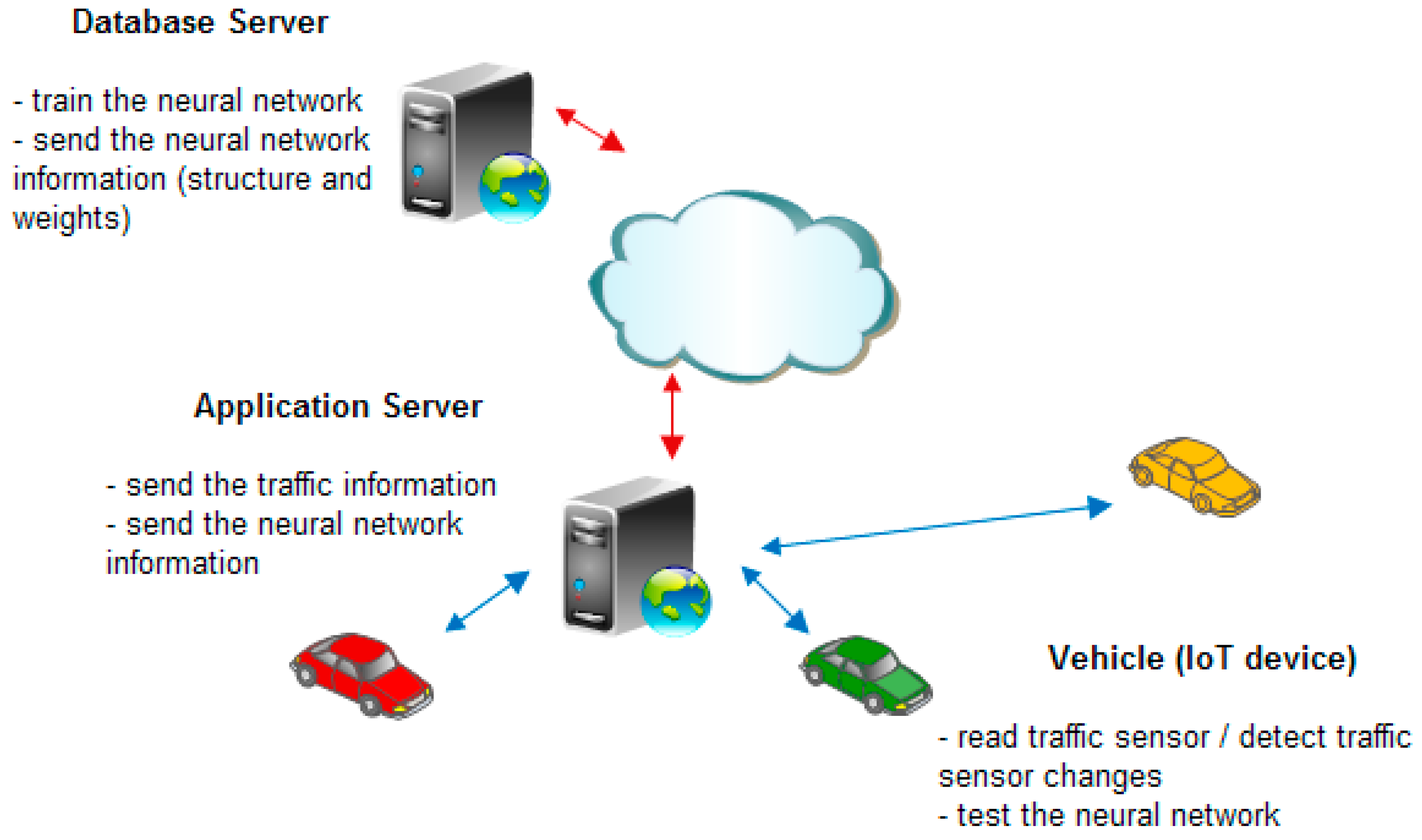
The system has two components: the developing phase and the operating phase. In the developing phase, the necessary sensor data (e.g., traffic information: number of vehicles that transit a specific node, their speeds) are collected by an application server that transmits this data to a database server which trains a neural network and returns the neural network parameters to the vehicles via an application server. In the operating phase, the neural network is tested, and a forecast is made as shown in Figure 1.

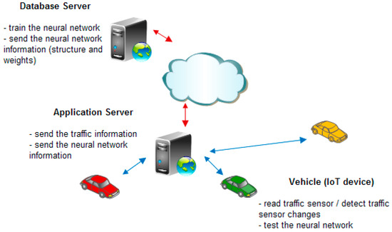
Figure 1. Traffic forecasting system architecture (adapted from [15]).

The system in Figure 1 is made up of a series of sensors, placed on the road, that take specific traffic information (number of cars and their average speed). Vehicles on the road can periodically read sensors or be informed of changes in sensor values. The vehicles can communicate with an application server that takes the same information from the sensors and transmits it to a database server that periodically trains a neural network with a specified architecture and determines its learnable parameters. The type of neural network and these parameters are transmitted back to the application server which transmits them to the vehicles.

According to the chosen scenario, the vehicles can read the sensors and run a program that tests the neural network, with the parameters taken from the application server, to predict the traffic and choose an optimal route. The prediction is more accurate if the vehicles use the values from the sensors as input to the neural network, but the load on the communication network is higher. On the other hand, reading the sensors less often reduces the load on the communication network, but the neural network uses the predicted values as inputs and, therefore, the accuracy of the prediction is lower, because the predicted values can be different from the real traffic values. A compromise must be made between the load of the communication network connecting the vehicles, the application server, and the database server and the accuracy of the prediction.

In this work, we consider scenarios in which the vehicles transiting roads request information about the traffic load and can predict the traffic to choose a route as short as possible to decrease road congestion, the travel time, and amount of energy consumed [1,16].

This paper presents cases derived from the point of view of the reading mode of sensors according to the models found in real-time systems: time-triggered and event-triggered. These scenarios evaluate the load of the communication network connecting the system components (especially vehicles and sensors) to obtain a compromise between a reduced load of the communication network and the accuracy of the prediction.

Spatial–temporal interactions are captured by using graphs as reinforcements in a recurrent neural network. The training phase (implemented on the database server), with various inputs, which correspond to complex transport networks and in which various traffic information is taken, optimizes the parameters of the neural network that are used in the normal operation of the system (testing phase) implemented on the vehicle microcontroller.

On the database server, one can train several types of neural networks with different architectures and/or numbers of levels and with different hyperparameters. In this way, the space–time problem associated with a neural network based on graphs and used for traffic prediction can be comprehensively captured.

However, this article is more focused on evaluating the possibility of real-time implementation of the test phase on vehicles.

The information is taken at specific moments in time from an application server which periodically updates its information from a database server.

The duration of the readings from the application server must be as short as possible to reduce the network load and to allow many vehicles to transit the same roads.

Two scenarios are analyzed: one in which the traffic prediction is performed using a constant analysis duration in which the real information from the nodes is read for a short period, after which the traffic prediction is made using the results provided by the neural network. In the second scenario, the traffic changes in the nodes are detected and the real information from the nodes is read for a fixed duration and then the traffic prediction is made from the neural network information until the next detection of a change in the real traffic.

For system implementation, one can choose a solution consisting of a powerful system on a chip from Analog Devices (consisting of ADuCRF101 which integrates an ARM Cortex M3 MCU at 16 MHz clock and a RF transceiver ADF7024) as hardware and AD6LoWPAN (which is the 6LoWPAN—IPv6 over Low-Power Wireless Personal Area Networks, provided by Analog Devices) with IoT operating system Contiki version 4.8 as software.

To make a prediction, a Long Short-Term Memory (LSTM) neural network is involved. This type of recurrent neural network has been proven to have good results in sequence prediction and their parameters were validated by simulation in MATLAB.

All the necessary functions that implement the neural network are considered and evaluated to see if the entire system can perform in real time using a microcontroller.

Considering a wireless node network in which a very important goal is energy conservation, specific implementation of threads (such as starting/stopping radio communication) should be implemented. In such cases, the event-driven model—described by a finite state machine (FSM)—is used. To simplify the system development, the threads can be replaced by protothreads that can be written without having to design finite state machines [16].

Protothreads are a programming abstraction and they reduce the complexity of implementations of event-triggered systems by performing conditional blocking of event-triggered systems, without the overhead of full multi-threading systems. They are lightweight threads without their own stack. This is advantageous in memory-constrained systems, where a stack for a thread uses a large part of the available memory.

Protothreads are based on a low-level mechanism named local continuations that can be set (the CPUs are captured) or resumed. A protothread is a C function with a single associated local continuation. The protothread’s local continuation is set before a conditional blocking. If the condition is true, the protothread executes a return statement to the caller program. In the next instance, the protothread is running and the local continuation is resumed to the one that was previously set and causes the program to jump to the conditional blocking statement. The condition is re-evaluated and, if the condition is false, the protothread executes the function.

In this paper, we consider an IoT application that is implemented with Contiki operating system support. The Contiki OS is intended for networked, memory-constrained, and low-power wireless IoT devices. Contiki provides multitasking and has a built-in Internet Protocol Suite (TCP/IP stack) with low memory requirements.

The Contiki programming model is based on protothreads [17,18]. The operating system kernel invokes the protothread in response to an event (timers expired, messages posted from other processes, triggered sensors, incoming packets from a network neighbor node). In Contiki, the protothreads are cooperatively scheduled; therefore, the process must always explicitly yield control back to the kernel at regular intervals by using a special protothread to block waiting for events while yielding control to the kernel between each event occurrence. Contiki supports inter-process communication using messages passing through events.

2. The Graph Neural Network

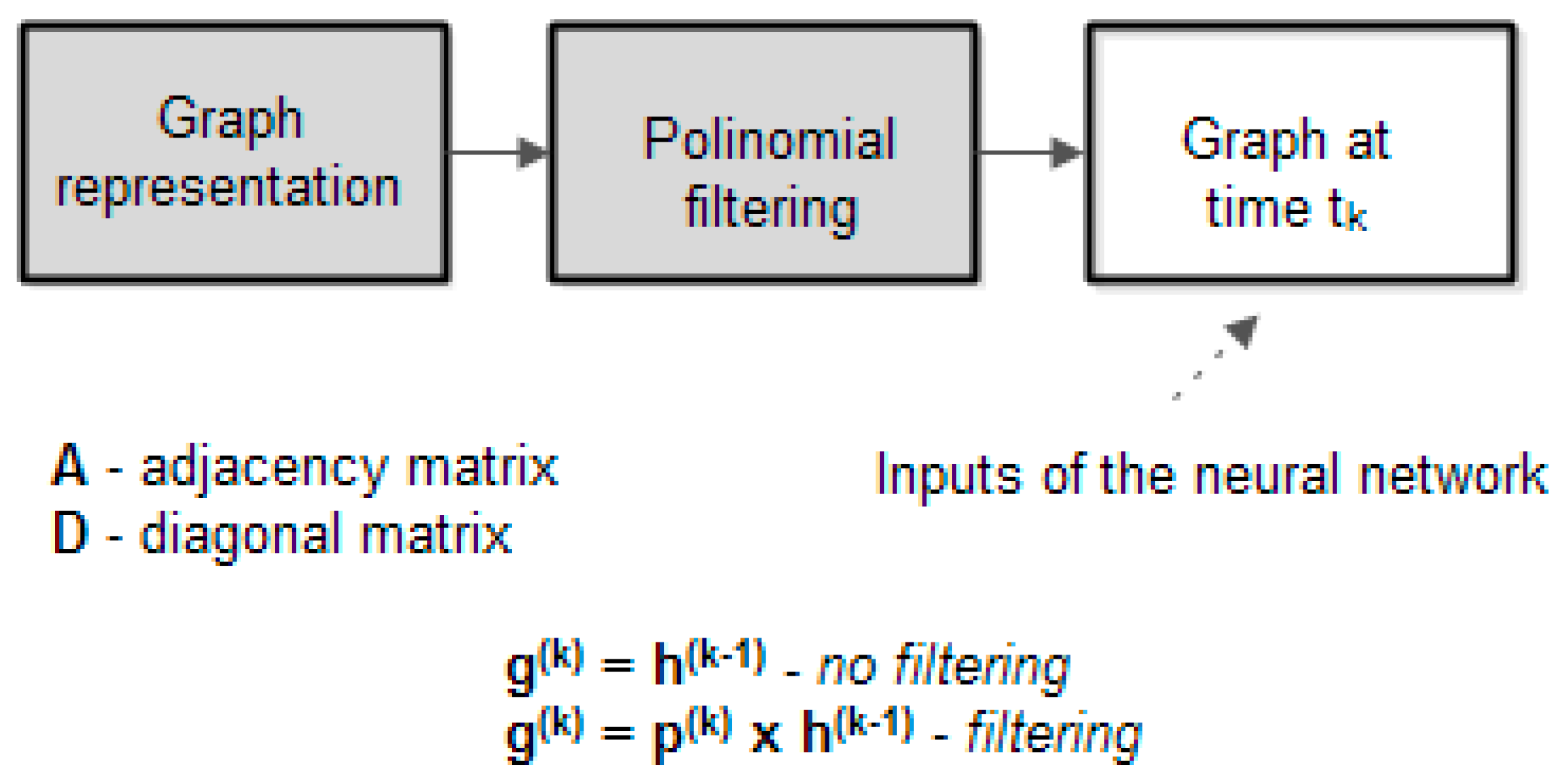
To use a graph as input in a neural network, the information associated with graph (e.g., node values, edges cost) should be converted to an appropriate form to be used as neural network input. Figure 2 illustrates how a graph can be represented with or without filtering. The greyed blocks transform the graph information, given as a vector (or matrix) that has on each line the data in a specific node. Each column represents specific information for a node. The way the graph is represented is presented below [19].

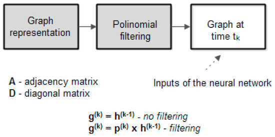
Figure 2. Graph representation and filtering (adapted from [15]).

Given a graph G, it is characterized by its adjacency matrix $A=[a_{ij}],\hspace{0.17em}i,\hspace{0.17em}j=1,\hspace{0.17em}\dots \hspace{0.17em},N$ where $a_{ij}$ indicates the existence of edge between nodes $i,\hspace{0.17em}j$ (1—presence, 0—absence) and $N$ is the number of nodes. Also, a node in graph G is characterized by the degree of the node which is the number of edges incident at the node. A diagonal matrix is defined as:

$$D=[d_{ij}],\hspace{0.17em}i,\hspace{0.17em}j=1,\hspace{0.17em}\dots \hspace{0.17em},N\hspace{0.17em}\hspace{0.17em}and\hspace{0.17em}\hspace{0.17em}{d}_{ij}=0,\hspace{0.17em}\hspace{0.17em}if\hspace{0.17em}i\ne j,\hspace{0.17em}\hspace{0.17em}{d}_{ii}={\displaystyle \sum _{k=1}^N{a}_{ik}}$$

A difference matrix $L\hspace{0.17em}=D-A$ is involved to build a polynomial as follows: $p(L)\hspace{0.17em}=\hspace{0.17em}{w}_0{I}_n\hspace{0.17em}+\hspace{0.17em}{w}_1{L}^{}\hspace{0.17em}+\hspace{0.17em}{w}_2{L}^2\hspace{0.17em}+\hspace{0.17em}\dots \hspace{0.17em}+w_d{L}^d$. The polynomial $p(L)\hspace{0.17em}$is a (n × n) matrix. We note the coefficients as vector $w\hspace{0.17em}=\hspace{0.17em}[w_k]\hspace{0.17em}\hspace{0.17em},\hspace{0.17em}k=0,\hspace{0.17em}1,\hspace{0.17em}\dots ,\hspace{0.17em}d$.

The polynomial $p(L)$ is used as a filter to calculate the neural network inputs (features). The generic algorithm for the training phase of the graph neural network is illustrated below (the vector $x$ represents the initial values in the nodes of the graph):

$$\begin{array}{l}Initialization\\ h^{(0)}=\hspace{0.17em}x\\ while\hspace{0.17em}(error\hspace{0.17em}\hspace{0.17em}>\hspace{0.17em}\mathrm{minimum}\hspace{0.17em}\hspace{0.17em}\mathrm{error}\hspace{0.17em})\hspace{0.17em}\hspace{0.17em}do\\ g^{(k)}\hspace{0.17em}=\hspace{0.17em}{p}^{(k)}\hspace{0.17em}\times \hspace{0.17em}{h}^{(k-1)}\hspace{0.17em}\\ h^{(k)}=\sigma (g^{(k)})\\ output=\hspace{0.17em}PREDICT(h^{(k)})\\ error=\hspace{0.17em}|output-\hspace{0.17em}\mathrm{target}|\\ do\hspace{0.17em}\hspace{0.17em}end\end{array}$$

The vector $w$ represents the polynomial coefficients and $x=\hspace{0.17em}[ x_1\hspace{0.17em}{x}_2\hspace{0.17em}\dots \hspace{0.17em}{x}_N ]$ represents the initial values in the graph’s nodes. The terms $x_i$ can be vectors if nodes have more information (e.g., numbers of vehicle stored by type or speed). The function $\sigma$ is the activation function (e.g., sigmoid). The sigmoid function gives the best results in our experiments, compared with the RELU function, but the computational time is greater. If terms $x_i$ are vectors, the activation function is applied elementwise. The superscript index k represents the discrete time index. In the above algorithm, PREDICT indicates a regression layer that predicts the output from previous inputs and the target represents the expected output.

The novelty of this article is the implementation of a traffic prediction system based on a neural network that uses graphs. The method with Laplacian polynomials was chosen as the graph representation method—and it was proven through experiments that this leads to better system performance. The author’s contribution consists in choosing the coefficients of the Laplacian polynomial (to have a good predictor and a small calculation time).

This algorithm is a generalization of some graph neural network algorithms. Therefore, the above-presented algorithm represents a general framework that can be used to obtain specific implementations of known graph-based neural networks [20]. For example, the equivalence with Graph Convolutional Networks (GCN) is proven below.

Consider a slight modification in the definition of adjacency matrix, as follows: $A=[\frac{a_{ij}}{{\displaystyle \sum _{j=1}^N{a}_{ij}}}],\hspace{0.17em}i,\hspace{0.17em}j=1,\hspace{0.17em}\dots \hspace{0.17em},N$. Then, the non-zero terms in the diagonal matrix $D\hspace{0.17em}$ are changed to $d_{ii}=1$.

If $w_i=0,\hspace{0.17em}i=\hspace{0.17em}2,\hspace{0.17em}3,\hspace{0.17em}\dots ,\hspace{0.17em}d$ then $p(L)\hspace{0.17em}=\hspace{0.17em}{w}_0{I}_n\hspace{0.17em}+\hspace{0.17em}{w}_1{L}^{}\hspace{0.17em}=\hspace{0.17em}{w}_0{I}_n\hspace{0.17em}+\hspace{0.17em}{w}_1(D-A)$ and $g^{(k)}\hspace{0.17em}=\hspace{0.17em}{p}^{(k)}\hspace{0.17em}\times \hspace{0.17em}{h}^{(k-1)}=$$w_0{I}_n\times \hspace{0.17em}{h}^{(k-1)}\hspace{0.17em}+\hspace{0.17em}{w}_1{I}_n\times \hspace{0.17em}{h}^{(k-1)}-w_{1}A\times \hspace{0.17em}{h}^{(k-1)}$$=(w_0+\hspace{0.17em}{w}_1)·\hspace{0.17em}{h}^{(k-1)}-w_{1}A\times \hspace{0.17em}{h}^{(k-1)}$ which represents the formulas for GCN.

3. The System Implementation

To forecast traffic, the Long Short-Term Memory (LSTM) neural network is an appropriate choice because the inputs are time series (the traffic values in each node in the graph that represents the transport road network and considers the spatial–temporal characteristics of the inputs).

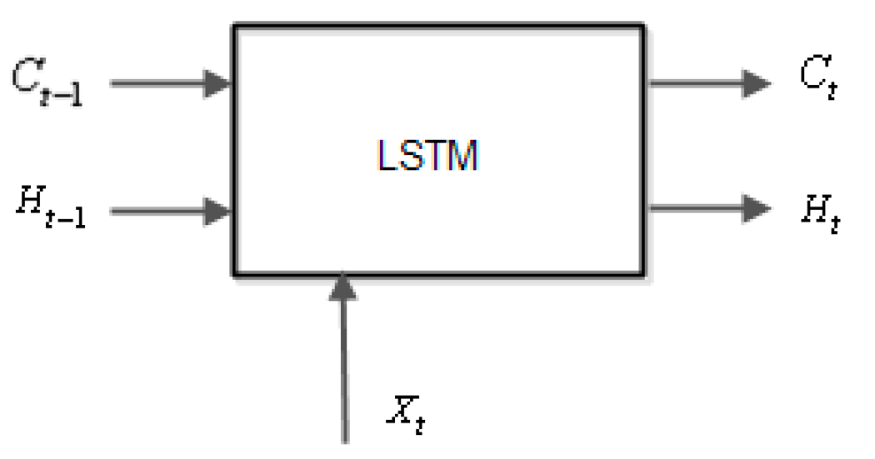
The LSTM network [19,21] is a recurrent neural network that processes input data by looping over time steps and updating its state and contains information stored over all the previous time moments and consists of several cells as in the Figure 3.

Figure 3. LSTM neural network cell.

At a given moment of time t, the input cell is $X_t$. The cell state at time t is $C_t$, and the output is $H_t$. The initial value of $C_{t-1}$ and $H_{t-1}$ at t = 0 is zero.

Assuming that $X_t$ and $H_t$ are $(M,1)$ vectors, $B_f,\hspace{0.17em}{B}_i,\hspace{0.17em}{B}_c,B_o\hspace{0.17em}$ are scalars, the weights $w_f,\hspace{0.17em}{w}_i,\hspace{0.17em}{w}_c,\hspace{0.17em}{w}_o$ are $(1,M)$ vectors, and the weight $w$ is a scalar with $M$ being the number of features (inputs in the neural network) and one output of the neural network, then the LSTM computations are the following relations:

$$F_t=\mathrm{sigmoid}({\displaystyle \sum _{i=0}^{M-1}[w_f(i)}·H_{t-1}(i)+w_f(i)·X_t(i)]+B_f)$$

$$I_t=\mathrm{sigmoid}({\displaystyle \sum _{i=0}^{M-1}[w_i(i)}·H_{t-1}(i)+w_i(i)·X_t(i)]+B_i)$$

$$C_t=F_t·C_{t-1}+I_t\tanh ({\displaystyle \sum _{i=0}^{M-1}[w_c(i)}·H_{t-1}(i)+w_c(i)·X_t(i)]+B_c)$$

$$O_t=\mathrm{sigmoid}({\displaystyle \sum _{i=0}^{M-1}[w_o(i)}·H_{t-1}(i)+w_o(i)·X_t(i)]+B_o)$$

$$H_t=O_t·\tanh (C_t)$$

At each time step, the neural network learns to predict the value of the next time step (the inputs are shifted by one time step) [22]. The sequence output is determined by a neural network regression layer. There are two methods of forecasting: open-loop and closed-loop forecasting. Open-loop forecasting predicts the next time step in a sequence using only the input data (true input from traffic sensors). The output sequence is predicted using several past input sequences. Closed-loop forecasting predicts using the previous predictions as input and does not require the true inputs’ values to make the prediction. To make a prediction for current time, this method uses the predicted value (past the neural network output) as input. The open-loop forecasting method has the disadvantage of a greater network load because each vehicle on the road more often reads the traffic sensors, but the traffic forecasting is more accurate. On the other hand, closed-loop forecasting requires fewer readings of traffic sensors (and reduces the network load), but the forecasting is less accurate and depends on neural network accuracy and graph filtering.

The proposed method takes into consideration two factors: the communication network load (how often the inputs in the neural network are updated) and the neural network performance (in terms of forecast accuracy). The two proposed scenarios follow the methods used in the real world: time-triggered systems or event-triggered systems. While time-triggered systems (scenario 1) are suitable for more predictable traffic, the event-triggered system is used for bursting-like traffic. The two scenarios are somewhat complementary (they are applied in different situations). However, the time-triggered system is simpler to implement and covers the event-triggered system. The communication network load is greater in the time-triggered system (scenario 1) than in the event-triggered system (scenario 2), but the neural network performance is better if it reads real inputs more often (like in scenario 1) instead of using the predicted outputs (as in scenario 2). This paper evaluates the traffic forecasting system performance, taking into consideration the trade-off between the communication network load and prediction accuracy of the neural network, and focuses on evaluating the feasibility of real-time implementation using microcontrollers.

The data set is a matrix with N rows (where each row represents a graph node which models the transport layer) and M columns (as discrete time). The matrix element is traffic load (as a percentage relative to a maximum value of traffic) or may be a vector which contains traffic load, average speed of vehicles that transit the node, average number and type of vehicles that transit the node, etc.

In this paper, we chose to use only the traffic load to not impose high restrictions for a real-time implementation on the vehicles’ microcontroller. Depending on the response time imposed, a more complex implementation can be achieved.

The obtained results show that the response occurs within seconds for a data set containing traffic load information. Our estimation is that if the data set contains more information, the response time should increase to tens of seconds which may be acceptable in certain systems.

Of course, the computation time increases greatly in the training phase if the data set is more complex, but this phase is implemented in the database server and is outside the scope of this paper.

Figure 4 shows the two proposed scenarios.

Figure 4. Traffic forecasting scenarios: [15]. (a) first scenario: constant analysis and reading intervals; (b) second scenario: input changes detection, constant reading interval.

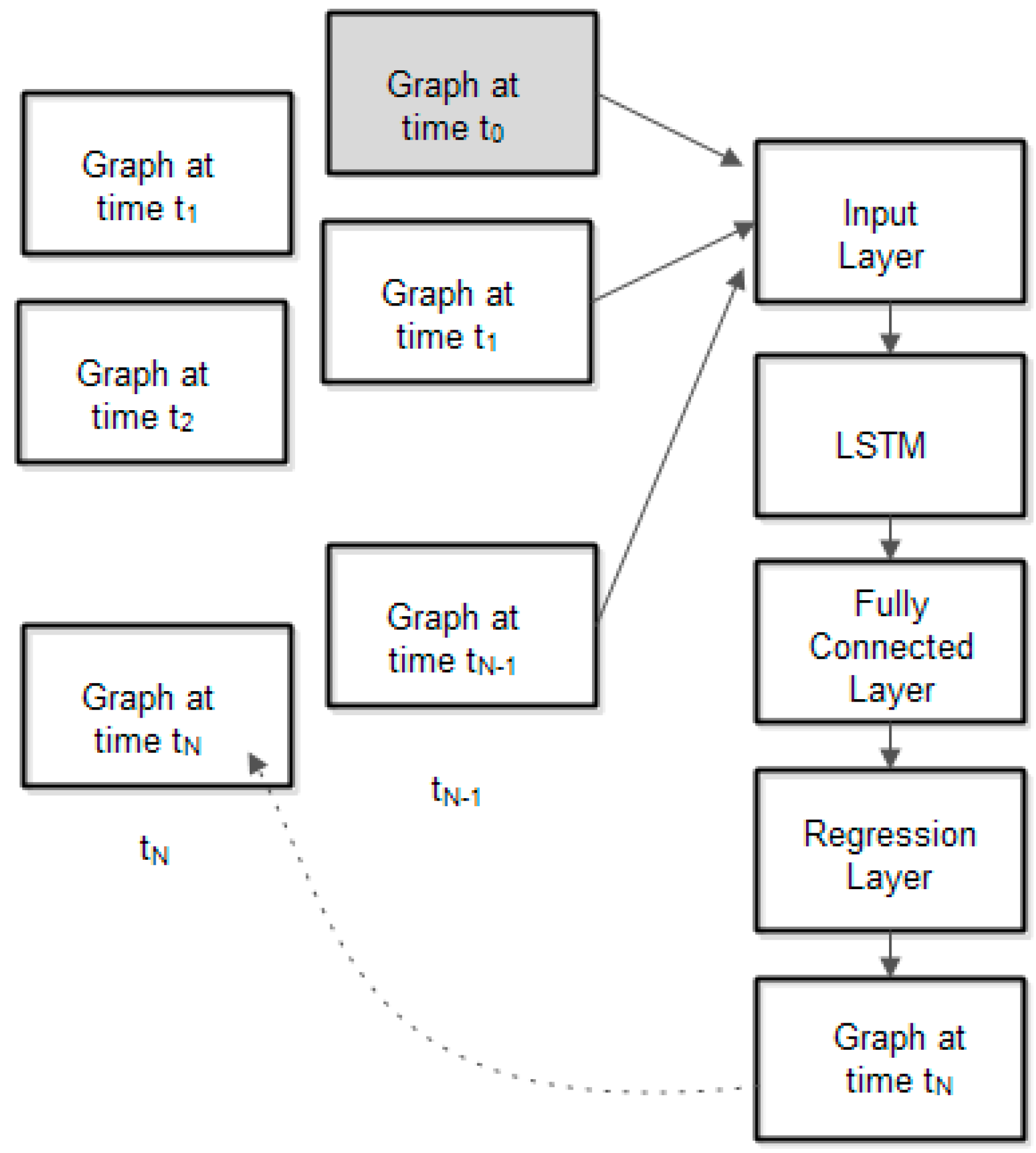
Figure 5 presents the neural network architecture with the following layers: input layer, LSTM layer, fully interconnected layer, and regression layer.

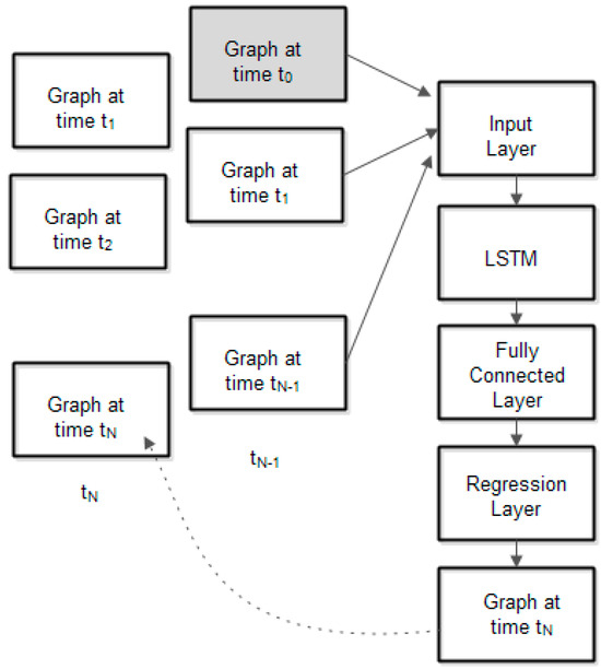
Figure 5. Traffic forecasting using graph-based neural network [15].

Fully connected layer computation is: $OUTPUT=w(i)·H_t$.

The neural network regression layer yields a predicted value by learning complex non-linear relationships.

The regression layer computes the half-mean-squared-error loss for regression tasks. For sequence-to-one regression networks, the loss function of the regression layer is the half-mean-squared-error of the predicted responses: $loss={\displaystyle \sum _{i=0}^{C-1}(t_i}-y_i{)}^2$. The output of the regression layer is the predicted sequence (that is, the predicted values in all nodes).

The data obtained from sensors can be traffic load (expressed as the ratio between the number of vehicles in the node and the maximum number of vehicles for all nodes), the average vehicle speed, the distance between nodes, etc. In our experiments, we consider the traffic load as node information. The neural network input is a matrix with N rows (number of nodes in graph) and M columns (discrete time). In future papers, we will extend the investigations, increasing the volume of node information.

The parameters of the neural network are determined by training it using an implementation in MATLAB (with traffic values like the real ones). Implementations were made for both scenarios and for both situations: without filtering or with filtering. The testing phase of the neural network (implemented on the vehicle’s microcontroller) uses parameters determined during the learning phase, which are optimized.

Future investigations will determine to what extent the optimization of neural network parameters (in the learning phase) can be implemented on microcontrollers, and how, in real time.

The training was performed using MATLAB and the parameters were experimentally chosen. A neural network with the following layers was used: sequence input with N dimensions (N numbers of nodes in the graph), LSTM with M hidden units, fully connected, and regression output (compute mean-squared-error). The testing phase was also implemented in MATLAB (only for validation) but it was implemented also using microcontrollers, following the procedure described in this article to evaluate the execution time and the accuracy. The main purpose of this article is to prove the feasibility of such an implementation (only for the testing phase).

The neural network training parameters are: 200 epochs with 7 observations each, 90% of observations used for training, and a learning rate of 0.001.

The neural network parameters have been optimized using the Regression Learner application in MATLAB. Training the neural network model in Regression Learner consists of two actions: train the neural network with a validation scheme and protect against overfitting by applying cross-validation and then train the neural network on full data, excluding test data. The application trains the model simultaneously with the validated model. To optimize the neural network’s learnable parameters, the cross-validation scheme is involved. The data set is partitioned into a few disjunct sets, and for each set, we train the neural network, evaluate model performance, and calculate the validation error over all sets. This method gives a good estimate of the predictive accuracy of the final learnable parameters trained. It requires multiple fits but efficiently uses all the data, so it can be used for small data sets. The Regression Learner exports the full optimized set of learnable parameters.

All the neural network’s learnable parameters are transferred from the database server to vehicles via the application server and they are used in the microcontrollers’ implementation for the testing phase.

4. Software Implementation

The framework for implementing the neural network application using microcontrollers is based on an Analog Devices wireless sensor network (WSN) for the Internet of Things (IoT), a flexible and modular solution used as a development platform. The hardware includes a base station node and several sensor nodes that support different sensors (the sensors can be connected in any combination). To implement the proposed framework, we use a WSN module [15,23,24,25] (EV-ADRN-WSN1Z_BUNCH) in each vehicle and the base node (EVAL-ADuCRF101MK) as the application server.

The nodes run a firmware provided by Analog Devices (AD6LoWPAN01 [15,23]—that is based on the Contiki OS) [26] as follows: the base node is configured as a border router to ensure communication between WSN nodes and a data server in another IP network, responsible for IPv6 Prefix propagation within the LoWPAN, and the WSN nodes are configured as sensor nodes (read traffic data and communicate with router). The original code provided with the evaluation platform in AD6LoWPAN01 [27] was modified to implement the proposed framework for neural network traffic forecasting applications.

The modified software has the flowcharts displayed in Figure 6, Figure 7 and Figure 8.

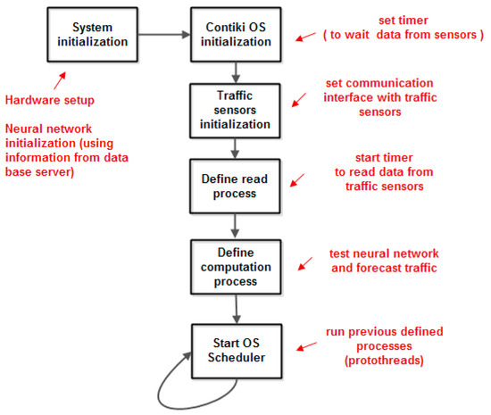
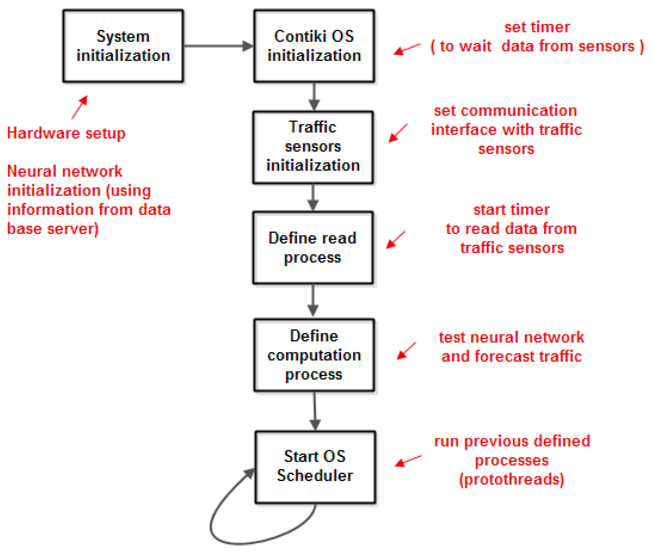
Figure 6. The overall framework flowchart (adapted from [23]).

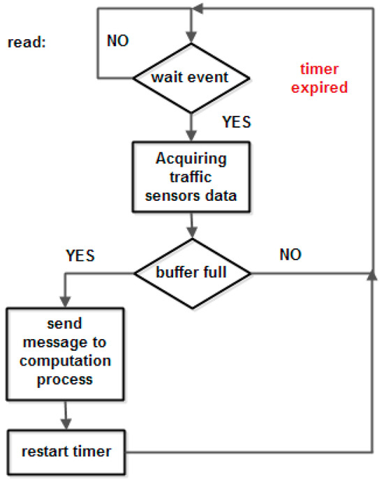
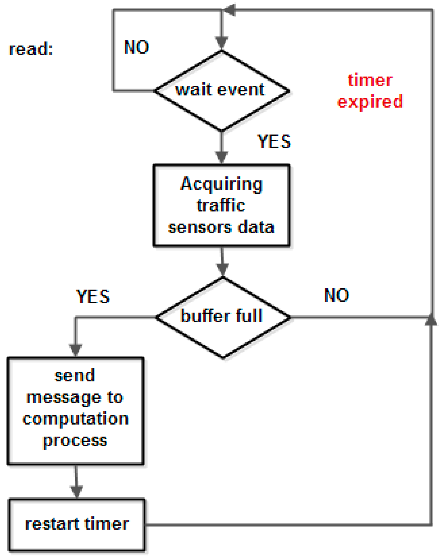
Figure 7. The read process flowchart (adapted from [23]).

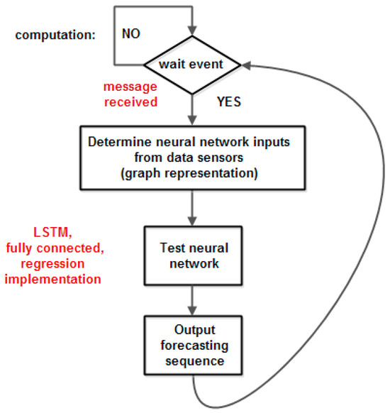
Figure 8. The computation process flowchart (adapted from [23]).

The algorithm was implemented using Contiki operating system primitives. The parameters of the neural network were initialized with parameters obtained in the training phase and the core of the Contiki operating system was initialized, which defines the processes of reading the sensors and updating the values from the input and processing graphs (implementation of the neural network). Both processes are executed when an event occurs: the expiration of a timer for the reading process and the filling of a buffer for the processing process. The timer associated with the reading process expires at the sampling rate of the sensors, and the buffer has a given length chosen in such a way that the processing is performed in real time. The execution of the two processes is cyclical.

In Figure 6, one can observe the main software modules of the proposed flowchart: hardware and software initialization, sensors initialization, and the two newly defined modules (implemented as protothreads), namely read process and computation process. The read process acquires traffic data sensors in a buffer at a configurable observation rate (in this paper, the observation rate is between 1 Hz and 10 Hz) and when the data buffer is full, it starts the computation process, as is illustrated in Figure 7.

The computation process waits for a message from the read process and then tests the neural network with the parameters and weights previously configured in the developing phase and makes a prediction. The flowchart of the computation process is shown in Figure 8.

The read process and computation process are run cyclically at a rate given by the filling of the data buffer.

The solution presented above involves the switching buffer technique [28]: two pairs of input and output buffers are switched to obtain a real time implementation (that is, without loss of input observations). Using an input buffer, it permits us to take a decision based on a large interval of time, not after a single observation. In this way, the decision accuracy is improved (for example, the decision may be taken considering the class that has a majority in the given interval of time). The sampling period may vary between tens of milliseconds and several seconds, and the input buffer maximum length may be chosen up to 100. In our evaluation, a sampling period of 1 s was chosen.

The necessary condition to have real-time implementation is:

$$Input\hspace{0.17em}buffer\hspace{0.17em}length\hspace{0.17em}\cdot Sampling\hspace{0.17em}period\ge Buffer\hspace{0.17em}computation\hspace{0.17em}\hspace{0.17em}time$$

We need to evaluate the computation time (that is, all the computation required by neural network test) to decide if the system runs in real time. One other issue is the numerical precision offered by the microcontroller to achieve the same prediction given by a floating-point implementation.

5. The Main Results

We consider a transport network consisting of 5–20 nodes (cities) with several routes. Each node measures the inbound and outbound traffic. A vehicle on a road (an edge) should forecast the traffic to choose a route that is less busy to increase the transportation energy efficiency. The neural network was trained using MATLAB [29] and it was tested using a C language implementation on microcontrollers on each vehicle [15,29]. The number of LSTM hidden layers is about 80 (our evaluation shows that increasing the number of layers does not improve the neural network performance).

The numbers of processor cycles of the function that implement LSTM relation are as follows: dot—857 cycles, sigmoid—164 cycles and tanh—59 cycles.

The execution time can be considered acceptable, as is shown in Figure 9.

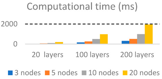
Figure 9. Computational time vs. number of layers and number of nodes in graph [15].

One can observe that the computational time is about 1 s for a neural network with about 100 layers. In Figure 9, the filtering is not considered, but in case of filtering, the execution time is increased by less than 10%.

Considering a reasonable assumption that a decision can be made in maximum of 60 s, this framework can be used for a traffic forecasting system with about five features (that is, five adjacent nodes in each node) and an input buffer up to 600 observations.

The above two scenarios were evaluated in terms of forecasting accuracy.

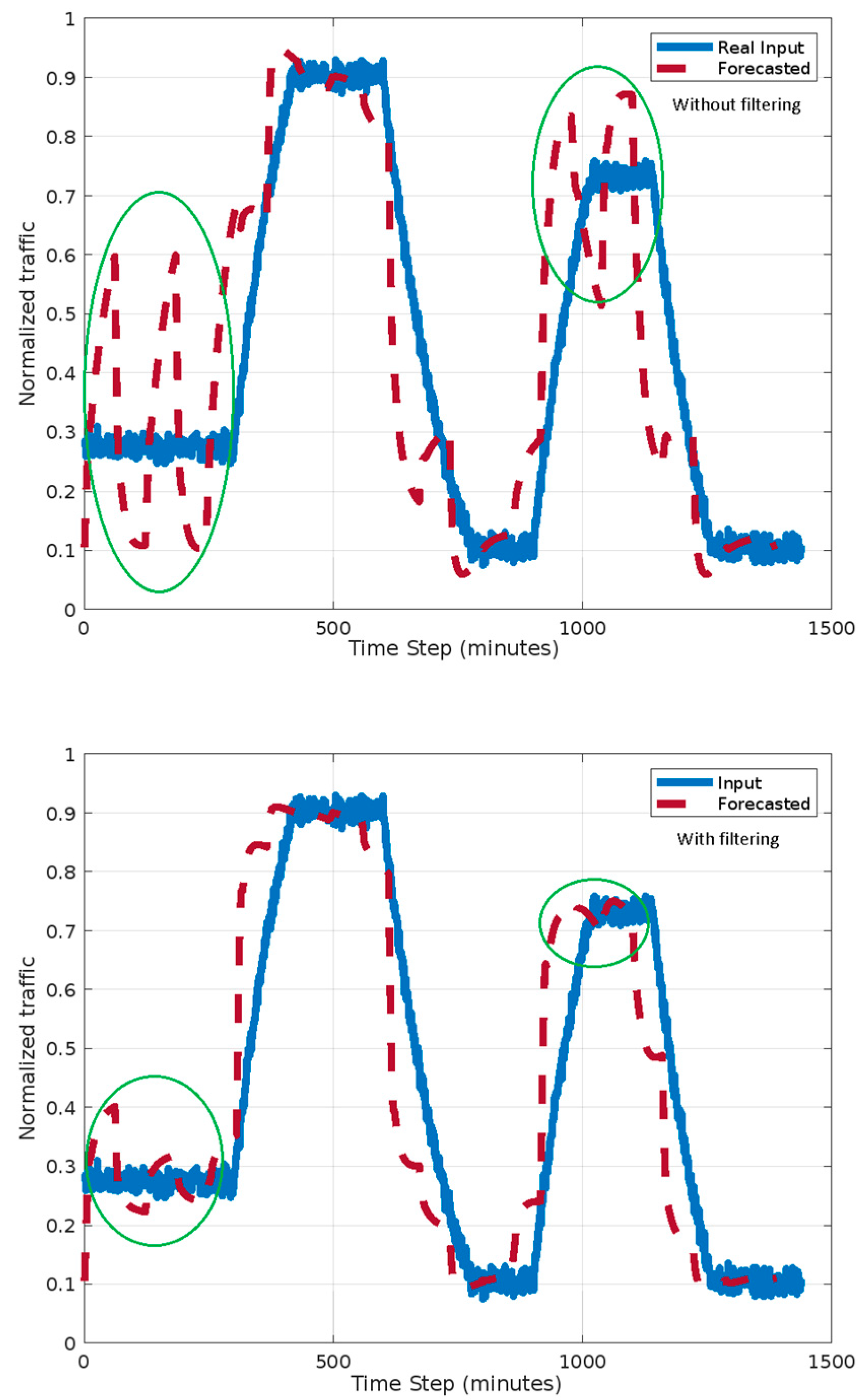
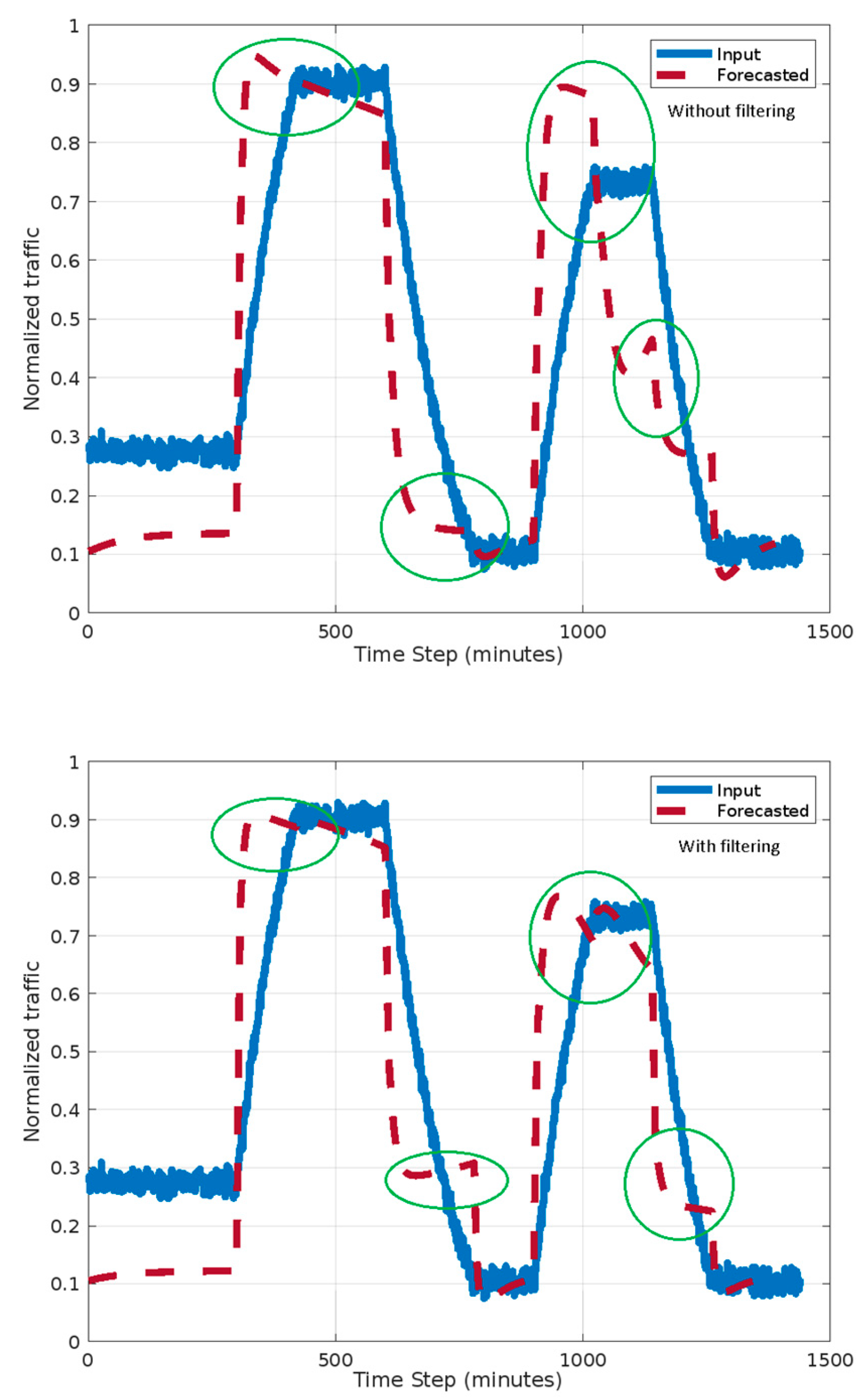
The first and second scenario results are shown in Figure 10 and Figure 11. The traffic is normalized to a maximum estimated traffic level.

Figure 10. Normalized forecasted traffic in first scenario [15].

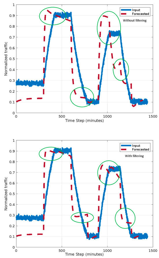
Figure 11. Normalized forecasted traffic in second scenario [15].

The circles in Figure 7 and Figure 8 indicate differences between the two scenarios both with and without filtering. One can observe that the forecast accuracy is better for the second scenario. The oscillations in forecasted traffic are eliminated if filtering is involved. This is due to a better choice of analysis interval.

To obtain a quantitative performance evaluation of the forecasting system, we compute the mean squared error as $MSE={\displaystyle \sum _{k=1}^N{[input(k)-forecasted(k)]}^2}$ and take the mean MSE value as a metric to determine the forecast precision. We also consider the load of the communication network as a ratio of the reading time of the sensors and the analysis time.

For the first scenario, the analysis interval is 60 min and for each analysis interval, the real inputs are read in the first 10 min. In the second scenario, after each detected traffic sensors’ change, the inputs are read for 10 s. In our experiments, a real input change occurs, on average, at 140 s. The readings’ intervals are smaller in the second scenario (less than 5 min per hour); therefore, the communication network load is twice as small as that in the first scenario. The detecting of changes increases the computational time by about 5%. In both scenarios, one can observe better accuracy if filtering is involved.

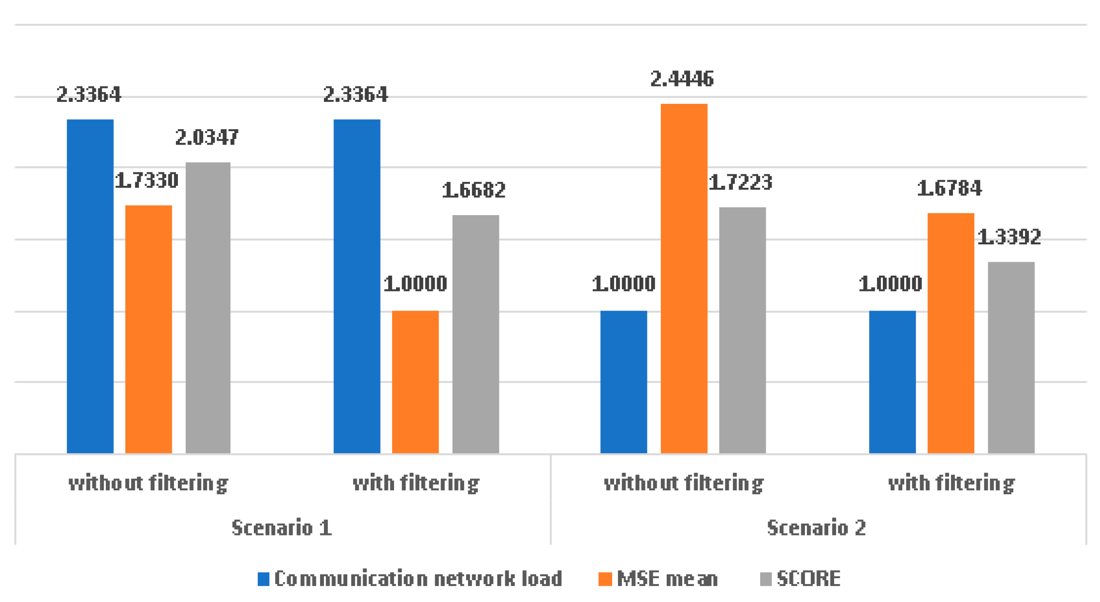
The global evaluation of the performance is given by a score calculated as an arithmetic mean between the MSE and the load of the communication network normalized to the load of the second scenario. Figure 12 indicates the overall performance of the forecasting system. In this figure, the communication network load was normalized to the load in the second scenario.

Figure 12. Overall performance (infinite precision) [15].

A lower score is better. One can observe that scenario 2 has better performance and filtering improves the performance in both scenarios.

Filtering improves accuracy in both scenarios.

Filtering leads to a greater improvement in the first scenario, which is simpler to implement. For the second scenario, which has a greater complexity, due to the necessity to detect significant changes in the input, filtering is useful, but the improvements are not so great as in the first scenario. Considering mean forecasting accuracy values, accuracy fluctuations, and communication network load with equal weights, the second scenario with filtering has better overall performance than the rest of the scenarios and the average overall improvement is about 27%. For both scenarios, an increase in reading time intervals leads to better accuracy, but the communication network load is increased. A trade-off between traffic forecasting accuracy and communication network load should consider determining the length of reading intervals.

6. The Numerical Quantization Evaluation

The neural network described in Section 3 was trained and tested in MATLAB to validate the traffic forecasting system and to compute the necessary parameters for real-time implementation using the previously described hardware and software platform. Using floating-point types on a microprocessor without a math coprocessor is inefficient, both in terms of code size and execution speed [15]. Therefore, one should consider replacing code that uses floating-point operations with code that uses integers, because these are more efficient. The Cortex M3 ARM architecture does not have a math co-processor or the operation required (specifically, an activation function should be implemented in floating-point implementations). Our implementation uses the C compiler support for floating point representation. In the representation of a signed 32-bit floating-point number, the exponent is 8 bits, and the mantissa is 23 bits. For a signed 64-bit floating-point number, the exponent is 11 bits, and the mantissa is 52 bits.

The functions dot product, sigmoid, and tanh were implemented in C language using 32-bit floating-point variable representations to determine the forecasting system accuracy with finite precision. The statistics of quantization errors (mean and standard deviation) for the dot product function are represented in Table 1. The quantization errors for this function are cumulative and, therefore, they depend on the number of features and number of classes. The statistics of quantization errors for the other mentioned functions are not dependent on the number of features. These statistics are depicted in Table 2.

Table 1. The dot product quantization error mean and standard deviation.

M	3	5	10	20
Error mean	0.011858	0.019425	0.038837	0.077625
Std. dev.	0.002957	0.004801	0.008251	0.015196

Table 2. The quantization error statistics.

	Function	Sigmoid	tanh
Statistic
mean		0.00102	0.00369
std		0.00110	0.00153

The LSTM quantization errors (one layer) are illustrated in Table 3.

Table 3. The LSTM quantization mean error and standard deviation.

M	3	5	10	20
Error mean	0.01627	0.01175	0.01185	0.01186
Std. dev.	0.01009	0.01087	0.01215	0.01226

The above-presented results show that in the implementation of the LSTM neural network as described in Section 3, using a microcontroller with 32-bit precision, the quantization error has no major impact on the neural network compared with using a personal computer (with infinite precision). The results in Figure 12 and Figure 13 consider the MSE mean normalized for the MSE mean in scenario 1 with filtering.

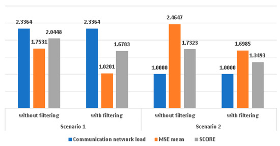
Figure 13. Overall performance (32 bits of precision) [15].

7. Conclusions

This paper introduces a general framework to implement a graph-based neural network and proposes an approach to forecasting traffic with good accuracy and reduced communication network load. Two scenarios were evaluated considering how often the vehicles read traffic sensors: periodically or change-triggered input reading. In both scenarios, a LSTM neural network is involved. This neural network predicts the information in the graph node (traffic and/or speed on edges from node) using as features real or predicted traffic information. Input data filtering is also evaluated. The main results show that filtering improves the forecasting accuracy in both scenarios with a slight increase in computational effort. The second scenario performs better than the first scenario but is sensitive to relatively slow changes in traffic.

Also, the paper analyzes and evaluates how a neural network can be implemented and tested using common microcontrollers. The impact of variables’ quantization on the prediction and the total system computation time were considered. The experiments show that the implementation of the LSTM neural network has very good performance. The accuracy does not decrease significantly due to the finite precision of the microcontrollers’ registers, and the implementation time is in real time for a reasonable number of features and classes in a traffic forecasting system. The proposed neural network framework is flexible and requires a small memory amount for coding. It can be used easily to realize various neural network models.

More sophisticated models of graph-based neural network testing using the proposed framework could be assessed.

References

- Shaygan, M.; Meese, C.; Li, W.; Zhao, X.; Nejad, M. Traffic prediction using artificial intelligence: Review of recent advances and emerging opportunities. Transp. Res. Part C Emerg. Technol. 2022, 145, 103921. [Google Scholar] [CrossRef]
- Available online: https://www.assemblyai.com/blog/ai-trends-graph-neural-networks (accessed on 23 March 2023).
- Jiang, W.; Luo, J. Graph neural network for traffic forecasting: A survey. Expert Syst. Appl. 2022, 207, 117921. [Google Scholar] [CrossRef]
- Rampášek, L.; Galkin, M.; Dwivedi, V.P.; Luu, A.T.; Wolf, G.; Beaini, D. Recipe for a general, powerful, scalable graph transformer. Adv. Neural Inf. Process. Syst. 2022, 35, 14501–14515. [Google Scholar]
- Kim, J.; Nguyen, D.; Min, S.; Cho, S.; Lee, M.; Lee, H.; Hong, S. Pure transformers are powerful graph learners. Adv. Neural Inf. Process. Syst. 2022, 35, 14582–14595. [Google Scholar]
- Liberis, E.; Lane, N.D. Neural networks on microcontrollers: Saving memory at inference via operator reordering. arXiv 2019, arXiv:1910.05110. [Google Scholar]
- Saha, S.S.; Sandha, S.S.; Srivastava, M. Machine Learning for Microcontroller-Class Hardware: A Review. IEEE Sens. J. 2022, 22, 21362–21390. [Google Scholar] [CrossRef] [PubMed]
- Lestari, D.; Muhammad, P.S.; Zaini, I.A. Implementation Artificial Neural Network on Microcontroller for Student Attention Level Monitoring Device Using EEG. In Proceedings of the 2020 6th International Conference on Science in Information Technology (ICSITech), Palu, Indonesia, 21–22 October 2020; pp. 57–61. [Google Scholar] [CrossRef]
- Lucan Orășan, I.; Seiculescu, C.; Căleanu, C.D. A Brief Review of Deep Neural Network Implementations for ARM Cortex-M Processor. Electronics 2022, 11, 2545. [Google Scholar] [CrossRef]
- Novac, P.-E.; Boukli Hacene, G.; Pegatoquet, A.; Miramond, B.; Gripon, V. Quantization and Deployment of Deep Neural Networks on Microcontrollers. Sensors 2021, 21, 2984. [Google Scholar] [CrossRef] [PubMed]
- Zhang, X.; Huang, C.; Xu, Y.; Xia, L.; Dai, P.; Bo, L.; Zhang, J.; Zheng, Y. Traffic Flow Forecasting with Spatial-Temporal Graph Diffusion Network. Proc. AAAI Conf. Artif. Intell. 2021, 35, 15008–15015. [Google Scholar] [CrossRef]
- Ye, J.; Zhao, J.; Ye, K.; Xu, C. How to Build a Graph-Based Deep Learning Architecture in Traffic Domain: A Survey. IEEE Trans. Intell. Transp. Syst. 2020, 23, 3904–3924. [Google Scholar] [CrossRef]
- Wang, Y.; Zheng, J.; Du, Y.; Huang, C.; Li, P. Traffic-GGNN: Predicting Traffic Flow via Attentional Spatial-Temporal Gated Graph Neural Networks. IEEE Trans. Intell. Transp. Syst. 2022, 23, 18423–18432. [Google Scholar] [CrossRef]
- Reyes, G.; Tolozano-Benites, R.; Lanzarini, L.; Estrebou, C.; Bariviera, A.F.; Barzola-Monteses, J. Methodology for the Identification of Vehicle Congestion Based on Dynamic Clustering. Sustainability 2023, 15, 16575. [Google Scholar] [CrossRef]
- Zoican, S.; Zoican, R.; Galatchi, D. Terrestrial Traffic Forecasting using Graph-based Neural Networks. In Proceedings of the 2023 16th International Conference on Advanced Technologies, Systems and Services in Telecommunications (TELSIKS), Nis, Serbia, 25–27 October 2023. accepted to publication. [Google Scholar]
- Akhtar, M.; Moridpour, S. A Review of Traffic Congestion Prediction Using Artificial Intelligence. J. Adv. Transp. 2021, 2021, 8878011. [Google Scholar] [CrossRef]
- Yu, B.; Yin, H.; Zhu, Z. Spatio-Temporal Graph Convolutional Networks: A Deep Learning Framework for Traffic Forecasting. In Proceedings of the Twenty-Seventh International Joint Conference on Artificial Intelligence, Stockholm, Sweden, 13–19 July 2018; pp. 3634–3640. [Google Scholar] [CrossRef]
- Dunkels, A.; Schmidt, O. Protothreads Lightweight, Stackless Threads in C; SICS Technical Report T2005:05; Swedish Institute of Computer Science: Kista, Sweden, 2005; ISSN 1100-3154. ISRN: SICS-T–2005/05-SE. [Google Scholar]
- Sanchez-Lengeling, B.; Reif, E.; Pearce, A.; Wiltschko, A. A Gentle Introduction to Graph Neural Networks. Distill 2021, 6, e33. [Google Scholar] [CrossRef]
- Available online: http://www.contiki-os.org/ (accessed on 23 March 2023).
- Available online: https://colah.github.io/posts/2015-08-Understanding-LSTMs (accessed on 23 March 2023).
- Graves, A. Long Short-Term Memory. In Supervised Sequence Labelling with Recurrent Neural Networks. Studies in Computational Intelligence; Springer: Berlin/Heidelberg, Germany, 2012; Volume 385. [Google Scholar] [CrossRef]
- Zoican, S.; Vochin, M.; Zoican, R.; Galatchi, D. Neural Network Testing Framework for Microcontrollers. In Proceedings of the 2022 14th International Conference on Communications (COMM), Bucharest, Romania, 16–18 June 2022; pp. 1–6. [Google Scholar] [CrossRef]
- IAR C/C++ Compiler User Guide. Available online: https://wwwfiles.iar.com/AVR/webic/doc/EWAVR_CompilerGuide.pdf (accessed on 23 March 2023).
- Available online: https://www.analog.com/media/en/technical-documentation/user-guides/UG-480.pdf (accessed on 15 February 2023).
- Adam, D. Contiki—A lightweight and flexible operating system for tiny, networked sensors. In Proceedings of the 29th Annual IEEE International Conference on Local Computer Networks, Tampa, FL, USA, 16–18 November 2004; pp. 455–462. [Google Scholar]
- Available online: https://datatracker.ietf.org/wg/6lowpan/ (accessed on 23 March 2023).
- Zoican, S.; Zoican, R.; Galatchi, D. Methods for Real Time Implementation of Image Processing Algorithms. Univ. Politeh. Buchar. Sci. Bull. Ser. C-Electr. Eng. Comput. Sci. 2015, 77, 137–148. [Google Scholar]
- Available online: https://www.mathworks.com/help/deeplearning/ug/time-series-forecasting-using-deep-learning.html (accessed on 23 March 2023).
Disclaimer/Publisher’s Note: The statements, opinions and data contained in all publications are solely those of the individual author(s) and contributor(s) and not of MDPI and/or the editor(s). MDPI and/or the editor(s) disclaim responsibility for any injury to people or property resulting from any ideas, methods, instructions or products referred to in the content. |
© 2024 by the authors. Licensee MDPI, Basel, Switzerland. This article is an open access article distributed under the terms and conditions of the Creative Commons Attribution (CC BY) license (https://creativecommons.org/licenses/by/4.0/).