Article

Pantograph–Catenary Interaction Prediction Model Based on SCSA-RBF Network

1
Department of Mechanics, Tianjin University, Tianjin 300072, China
2
State Key Laboratory of Nonlinear Mechanics, Institute of Mechanics, Chinese Academy of Sciences, Beijing 100190, China
*
Authors to whom correspondence should be addressed.
Appl. Sci. 2024, 14(1), 449; https://doi.org/10.3390/app14010449
Submission received: 27 November 2023 / Revised: 22 December 2023 / Accepted: 27 December 2023 / Published: 4 January 2024

Abstract

:
As a traditional numerical simulation method for pantograph–catenary interaction research, the pantograph–catenary finite element model cannot be applied to the real-time monitoring of pantograph–catenary contact force, and the computational cost required for the multi-parameter joint optimization of the pantograph–catenary system with the finite element model is very high. In this paper, based on the selective crow search algorithm–radial basis function (SCSA-RBF) network, the time-domain signal of the panhead acceleration, which can be obtained in real-time through non-contact test technology, is taken as the boundary condition to directly solve the pantograph dynamic equation and a data-physics coupling model that can quickly predict the pantograph–catenary interaction is proposed. The prediction model is trained and verified using the dataset generated through the finite element model. Furthermore, the prediction model is applied to the multi-parameter joint optimization of six pantograph dynamic parameters and nine pantograph dynamic parameters, considering nonlinear panhead stiffness, and optimization suggestions under various speeds and filtering frequencies are given.

1. Introduction

The “CR450 technological innovation project” of China State Railway Group proposes that the operating speed of electric multiple units (EMUs) should be 400 km/h, and the maximum speed should be 450 km/h [1]. For most completed high-speed rail lines, since the costs arising from changes in catenary parameters could be high, optimizing pantograph parameters to improve the current collection quality of the pantograph–catenary system at higher speeds, i.e., 400 km/h and above, is a more feasible and effective method.
The numerical simulation of pantograph–catenary interaction is usually based on the finite element method (FEM) [2,3,4]. The classic approach is to simplify the pantograph to a reduced model consisting of only a few lumped masses and spring-damper elements and construct a model of the catenary that consists of more than 10,000 finite element elements. With the objective of improving pantograph–catenary interaction performance, the optimization of pantograph–catenary parameters may include 1 to more than 10 decision variables and involve thousands or even tens of thousands of simulation cases. If the pantograph–catenary finite element model is used, hundreds of thousands of core hours are needed to solve a single set of pantograph–catenary parameter optimization problems. For different optimization scenarios, such as different running speeds on different operating lines and optimization scheme designs for different types of pantographs, it is often necessary to solve multiple sets of pantograph–catenary parameter optimization problems, which results in huge computational costs. Therefore, it is an urgent issue to improve the numerical calculation efficiency and reduce the computational cost.
The vast majority of the elements in the pantograph–catenary finite element model are located in the catenary model. The catenary finite element model adopts the geometric and material parameters of the real catenary, with a total structural length exceeding a thousand meters, containing tens of spans with repetitive structures. Rod or beam elements are often used to simulate contact wires, messenger wires, and stitch wires. The nonlinear spring elements, which only bear tension, are often used to simulate the droppers. The spring-lumped mass systems are used to simulate the steady arms, and the lumped masses are used to simulate various clamps [2,5,6,7].
To reduce the computational cost of numerical simulation, methods that can be adopted include improving the finite element model of the catenary, simplifying the physical model of the catenary, and constructing the surrogate model of pantograph–catenary interaction. Firstly, for the finite element model, the number of meshes can be reduced, or its nonlinear terms can be ignored. With the moving mesh method, finer meshes are set around the area near the contact point of the contact line, and coarse fixed meshes are set in the other areas to reduce the number of finite element elements of the catenary model. At 300 km/h and below, the relative error of the obtained time-domain signal of the contact force is lower than 7%, and the computational cost is reduced to 1/3 of that before mesh optimization [8]. Correction forces are used to eliminate the nonlinear stiffness term arising from the slackening of the dropper or the loss of pantograph–catenary contact. The solution process is divided into the online stage and the offline stage. The large matrix in the finite element model is pre-decomposed using LU factorization, which can considerably decrease computational cost while ensuring reasonable calculation accuracy [9,10].
Secondly, the structure of the catenary can be simplified with an equivalent method. However, the results of the simplified catenary model have a relatively large error compared with those of the finite element model. One approach is to simplify the catenary to a spring-mass system with time-varying stiffness, in which the spring stiffness is expressed as a sinusoidal function with the time of the pantograph running in a span as a period [11] or is directly given by the displacement response of the catenary finite element model under a constant static force [12]. The relative error of the contact force at 350 km/h and below obtained through the two models is up to 20~80% [13]. An alternative approach is to simplify the catenary to a periodically spring-supported string model. For example, a three-span-long string model supported by four springs, in which the relative error of the first natural frequency is 28% [14], or an infinite string model with viscoelastic support, in which the relative error of the standard deviation of contact force (SDCF) at 350 km/h and below is up to 32% [15,16].
Thirdly, the surrogate model of the pantograph–catenary interaction performance characterization parameters can be established by generating the data set containing several pantograph–catenary interaction cases through the finite element model. In the surrogate model, the computational cost drops several orders of magnitude at the expense of ignoring the dynamic process. For example, the quadratic function relationship between the SDCF at 305 km/h and the six pantograph parameters is established [17]. The surrogate model to represent the relationship between the SDCF at 350 km/h and six pantograph parameters, three dropper distribution parameters, three dropper length parameters, and three preload parameters is established, and the relative error of the model is less than 6.3% [18] The surrogate model to represent the relationship between the five contact force statistics parameters and running speed, static lifting force, and nine catenary parameters is established, and the determination coefficient of the model is 0.969 [19]; the surrogate model to represent the relationship between the time-domain signal of contact force and running speed in the range of 250~350 km/h and six catenary parameters is established, and the probability of the relative error of the SDCF surrogate model being lower than 4.6% is 99.73% [20]; the surrogate model to represent the relationship between the SDCF and running speed in the range of 250~450 km/h and six pantograph parameters is established, and the determination coefficient of the model is 0.996 [21].
Based on the verified pantograph–catenary finite element model, a dataset of 4000 pantograph–catenary interaction cases was generated in the whole speed range of 250~450 km/h. Combined with the selective crow search algorithm–radial basis function (SCSA-RBF) network, based on the time-domain signal of the panhead acceleration and the pantograph dynamic equation, and considering the pantograph–catenary interaction dynamic process, a data-physics coupling model that can accurately and quickly predict the pantograph–catenary interaction was proposed and applied to the multi-parameter joint optimization of pantograph dynamic parameters.

2. Pantograph–Catenary Finite Element Model [7]

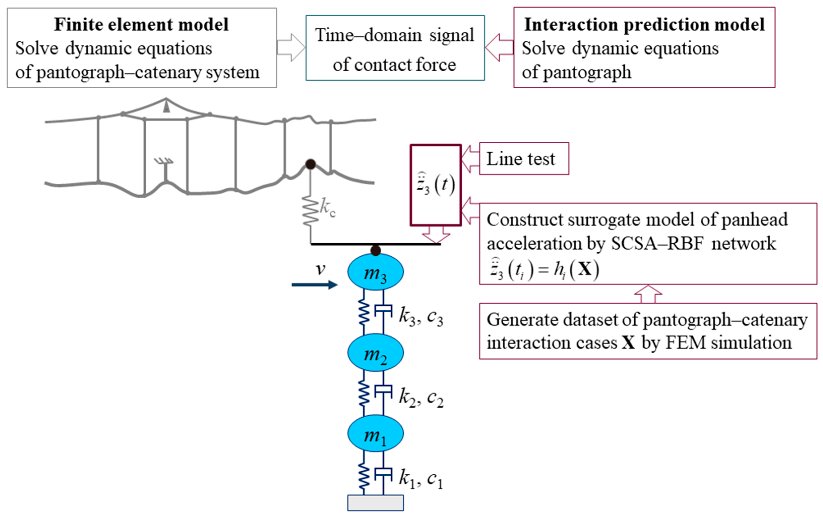
During the dynamic analysis of the pantograph–catenary system, the pantograph is usually equivalent to a three-mass model with three vertical degrees of freedom (DOFs). The pantograph dynamic equation is as follows:
m 3 0 0 0 m 2 0 0 0 m 1 z ¨ 3 t z ¨ 2 t z ¨ 1 t + c 3 c 3 0 c 3 c 3 + c 2 c 2 0 c 2 c 2 + c 1 z ˙ 3 t z ˙ 2 t z ˙ 1 t + k 3 k 3 0 k 3 k 3 + k 2 k 2 0 k 2 k 2 + k 1 z 3 t z 2 t z 1 t = F c t F 2 F 1
where mn, kn, and cn are the equivalent mass, stiffness, and damping, respectively. Fn is the lifting forces, zn(t), z ˙ n t and z ¨ n t are the vertical displacement, velocity, and acceleration, respectively. Subscripts n = 3, 2, and 1 represent the three lumped masses equivalent to the vertical vibration of the panhead, vertical bending vibration of the upper frame, and rotation of the frame, respectively. Fc(t) is the contact force.
A finite element model of the 30 spans two-dimensional stitched catenary system was established, referring to the geometric and material parameters of the actual catenary. The model included contact wires, messenger wires, stitch wires, droppers, steady arms, and various clamps. The contact wires, messenger wires, and stitch wires were treated as slender rod models with prestress due to their large length in comparison to their cross-sectional sizes and significant pretension. The element length for these wires was set at 0.2 m. The droppers were equivalent to nonlinear spring elements that only bear tension, and each dropper was only divided into one element. The steady arms were equivalent to a spring-lumped mass system, and each steady arm was only divided into one spring-lumped mass system. Each clamp was equivalent to a lumped mass. The proportional damping coefficients of the catenary dynamic system, α and β, were set to 1.25 × 10⁻² s−1 and 1.00 × 10⁻⁴ s, respectively. Based on the above assumptions, the dynamic equations of the catenary could be obtained. The penalty function method, with a contact stiffness of kc = 50,000 N/m, was used to simulate the coupling behavior between the panhead strips and contact wire, and the dynamic equations of the interaction of the pantograph–catenary system could be accordingly obtained. By combining the above equations, the dynamic equation of the pantograph–catenary system could be obtained. The maximum integration step of time was set to 0.00167 s, and the interval time for output was set to 0.005 s; that is, the sampling frequency was set to 200 Hz. At a given operating speed, pantograph–catenary parameters, and contact stiffness, the time-domain signals of the contact force and panhead acceleration, namely Fc(t) and z ¨ 3 t , were calculated using Ansys 19.2® commercial software.
The FEM calculated values of the above pantograph–catenary finite element model (Figure 1) have been verified using the measured data from line tests on the Datong-Xi’an High-speed Railway Line [7] and the trade standard EN50318:2018 [22,23]. The computational cost of the pantograph–catenary finite element model was about 10 core hours when calculating a single pantograph–catenary interaction case.

3. Pantograph–Catenary Interaction Prediction Model

3.1. Model Architecture

In the investigated pantograph–catenary system, the decision vector X = {v, m3, m2, m1, k3, k2, c1}T composed of the running speed and six pantograph equivalent parameters was variable, while the other three pantograph equivalent parameters, catenary parameters, and contact stiffness were given as constants. According to engineering practice, the value range for each decision variable in X was determined. Using the Latin hypercube sampling method [24], three disjoint sets, A, B, and C, were composed in a seven-dimensional sample space of X. Based on the pantograph–catenary FEM model, dynamic calculations were carried out to obtain the FEM calculated values of the time-domain signal of the panhead acceleration z ¨ 3 t , the time-domain signal of the contact force Fc(t), and the SDCF σ.
The SCSA-RBF network [21] was used to construct a surrogate model of the panhead acceleration at time ti, with set A as the training set and set B as the validation set. Minimizing p = 1 N p 1 R 2 p / N p of the validation set is the optimization objective. Among them, R 2 p is the determination coefficient between the model-predicted value and the FEM-calculated value of the time-domain signal of the panhead vertical acceleration of the validation set sample Xp. The closer R 2 p is to one, the smaller the error between the model-predicted value and the FEM-calculated value; p = 1, …, and Np, where Np is the number of samples in the validation set; ti = 0.1i/v (I = 0, 1, …, and 11,001). The SCSA-RBF network is a radial basis function network (RBF) [25] trained by the selective crow search algorithm (SCSA). SCSA introduces a roulette search operator [26] based on a crow search algorithm [27], which effectively improves the solution accuracy and convergence speed compared with the crow search algorithm. Using A∪B as the training set, the final surrogate model z ¨ 3 t i = h i X was obtained.
For any X, z ¨ 3 t i was obtained through the above surrogate model. The panhead vertical acceleration z ¨ 3 t j at time tj = 0.005(j – 1) (j = 1, 2, …) was calculated using the cubic spline interpolation method. Based on the Simpson formula and the trapezoidal quadrature formula, combined with the initial conditions of z ˙ 3 0 = 0 and z 3 0 = 0 , the vertical velocity and vertical displacement of the panhead at tj+1 can be obtained.
z ˙ 3 t j + 1 = z ˙ 3 t j + 0.0025 z ¨ 3 t j + z ¨ 3 t j + 1
and
z 3 t j + 1 = z 3 t j + 0.005 5 z ˙ 3 t j + z ˙ 3 t j + 1 / 6 + 0.005 2 3 z ¨ 3 t j + z ¨ 3 t j + 1 / 12 .
Taking z ¨ 3 t j , z ˙ 3 t j , and z 3 t j as the boundary conditions, combined with the initial conditions, the pantograph dynamic Equation (1) can be solved to obtain the predicted value of the pantograph–catenary contact force F c t j . In the numerical calculation, the calculation parameters and the dynamics iteration steps are the same as those in Section 2. In this paper, the above prediction method for the time-domain signal of the dynamic response for the pantograph–catenary system, based on the SCSA-RBF network and considering the physical process of pantograph–catenary interaction, is referred to as the pantograph–catenary interaction prediction model (Figure 2).
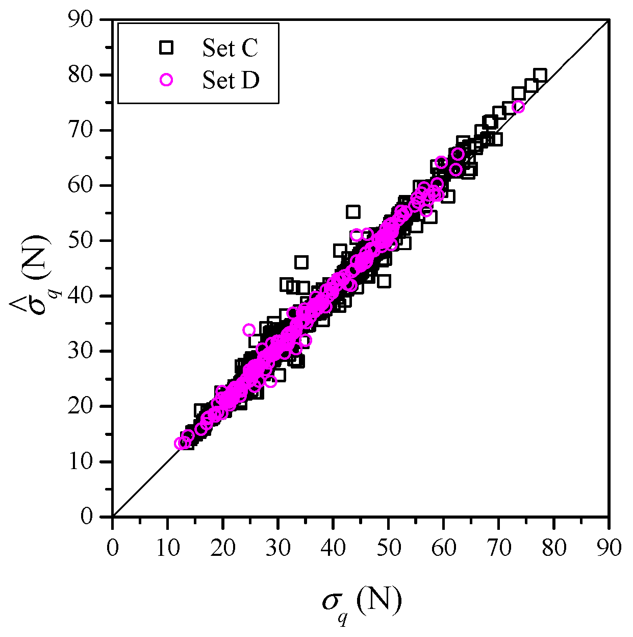
To evaluate the generalization ability of the pantograph–catenary interaction prediction model, set C was designated as the test set to calculate the determination coefficient between the model-predicted value and the FEM-calculated value of the time-domain signals of the panhead vertical acceleration and pantograph–catenary contact force in the test set. The average values and the interval within the probability of 0.95 of these coefficients were obtained. According to the trade standard EN50367:2020 [28], the SDCF, denoted as σ, is a critical index to evaluate the current collection quality and represents the oscillation degree of the time-domain signal of the contact force. Based on the model-predicted value F c t j and the FEM-calculated value Fc(tj) of the time-domain signal of contact force, their standard deviation σ ^ q and σq were calculated. In addition, the determination coefficient between the σ ^ q and the σq was calculated, and the interval of the model errors σ ^ q σ q within the probability of 0.95 was obtained. Among them, the subscript q represents the sample Xq (q = 1, …, and Nq) in the test set.

3.2. Consideration of a Piecewise Linear Panhead Spring

Three parameters, k31, k32, and S0, will be involved if the panhead spring exhibits piecewise linear stiffness. When the spring force S(t) < S0, the spring stiffness is k31; when S(t) ≥ S0, the spring stiffness is k32. Similarly, the ranges of the three decision variables were determined according to engineering practice. Then, the decision vector was extended to Y = {v, m3, m2, m1, k31, k32, S0, k2, c1}T.
It was assumed that the dynamic characteristics of the nonlinear panhead spring are equivalent to that of a linear spring over the entire analysis period, and the equivalent stiffness k3 could be expressed as
k3 = ηk31 + (1 – η)k32
where η represents the percentage of the sum of time when the spring stiffness is expressed as k31 in the total time. The following steps were taken to make Y equivalent to X: (1) Take X0 = {v, m3, m2, m1, k30, k2, c1}T, that is, k30 = k31 and r = 0. (2) Based on the pantograph–catenary interaction prediction model in Section 3.1, the predicted value of the vertical displacement of panhead and the second lumped mass, denoted as z 3 t j and z 2 t j , and the predicted value of the spring force S t j = k 3 r z 2 t j z 3 t j were obtained. Count the number of time sampling points with S t j < S 0 in the whole analysis period and divide it by the total number of time sampling points to obtain η, set k3r+1 = ηk31 + (1 – η)k32. (3) If |k3r+1k3r| < 1 N/m, X = Xr, and stop iteration; otherwise, set r = r + 1, Xr = {v, m3, m2, m1, k3r, k2, c1}T, and repeat step (2).
For the equivalent decision vector X, the same method in Section 3.1 was used to obtain the boundary conditions z ¨ 3 t j , z ˙ 3 t j , and z 3 t j . Combined with the initial conditions, the dynamic equation (1) of the three-mass model of the pantograph was solved to obtain the model-predicted value of the pantograph–catenary contact force F c t . In the process of solving the dynamic equation, at each time integration point, if S(t) < S0, replace k3 in Equation (1) with k31; if S(t) > S0, replace k3 with k32.
Hereinafter, the pantograph–catenary interaction prediction model was extended to the case of a piecewise linear panhead spring. Furthermore, the Latin hypercube sampling method was used to draw set D in a nine-dimensional sample space of Y. Set D was considered as the test set to evaluate the generalization ability of the pantograph–catenary interaction prediction model in the case of a piecewise linear panhead spring.

3.3. Performance Evaluation of Prediction Model

The catenary parameters of the stitched catenary of Datong-Xi’an High-speed Railway Line [7] were adopted and set k1 = 74 N/m, c3 = 50 N∙s/m, and c2 = 10 N∙s/m. Each decision variable in X used the same value range as in our team’s previous article [21]. In the decision vector Y, the value range of k31 and k32 is <4000, 14,000> N/m, and the value range of S0 is <130, 520> N. The sample sizes of sets A, B, C, and D were 2200, 900, 900, and 200, respectively.
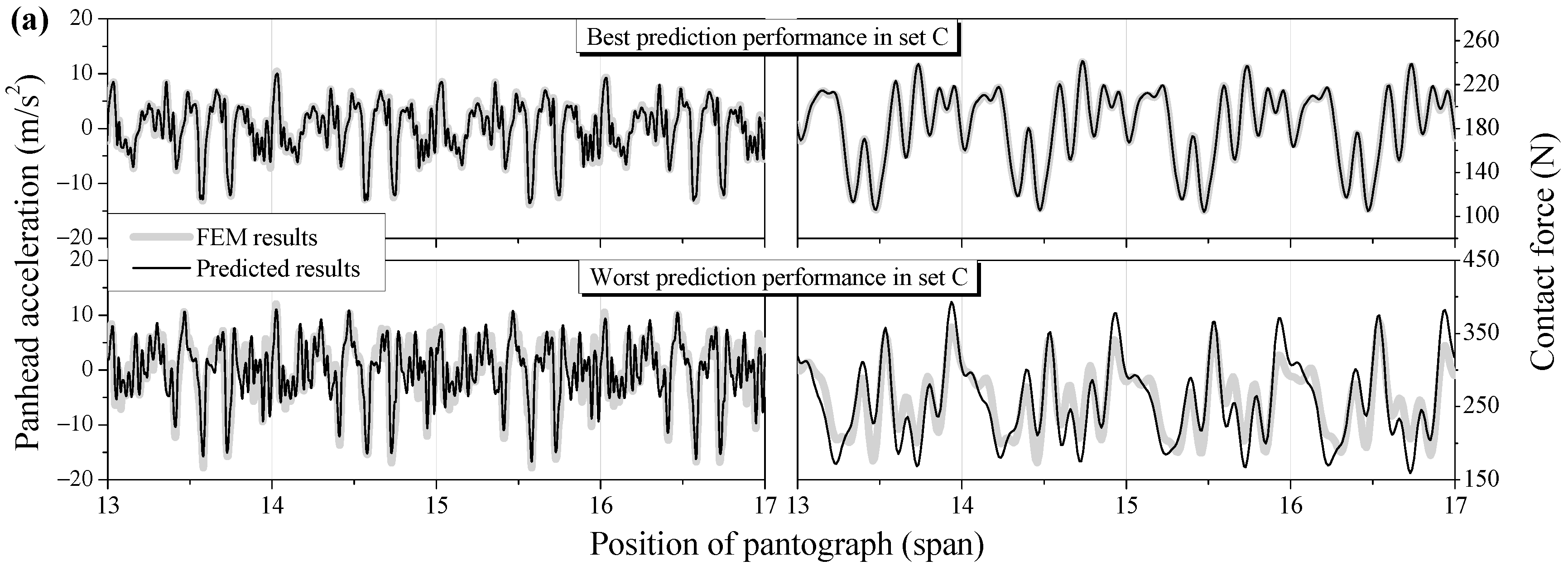
For set C with linear panhead stiffness, Figure 3a shows the time-domain signals of the panhead acceleration and the pantograph–catenary contact force of the samples with the best and worst prediction effect among them. Figure 4a shows the distribution of the determination coefficient of the time-domain signals and model errors of all samples. The relevant statistical values are given in the second row of Table 1. It can be seen that the probability density of the determination coefficient between the model-predicted value and FEM-calculated value of the two kinds of time-domain signals presents a left-skewed distribution. The intervals within the probability of 0.95 of them are (92.8%, 100%> and (91.0%, 100%>, respectively, which means most of the values are greater than their mean values of 97.7% and 97.4%. Obviously, for the sample with the maximum determination coefficient, the model-predicted results of the two kinds of time-domain signals almost coincide with their FEM results. Even for the sample with the minimum determination coefficient, the prediction accuracy of the two kinds of time-domain signals is also high. In addition, the model-predicted values of the SDCF in these samples are basically the same as those of the FEM-calculated value (□ in Figure 5), and the determination coefficient between them is 98.2%. The probability density distribution of model errors is approximately symmetric, and the interval within the probability of 0.95 of the model errors is <−2.35, 3.60> N.
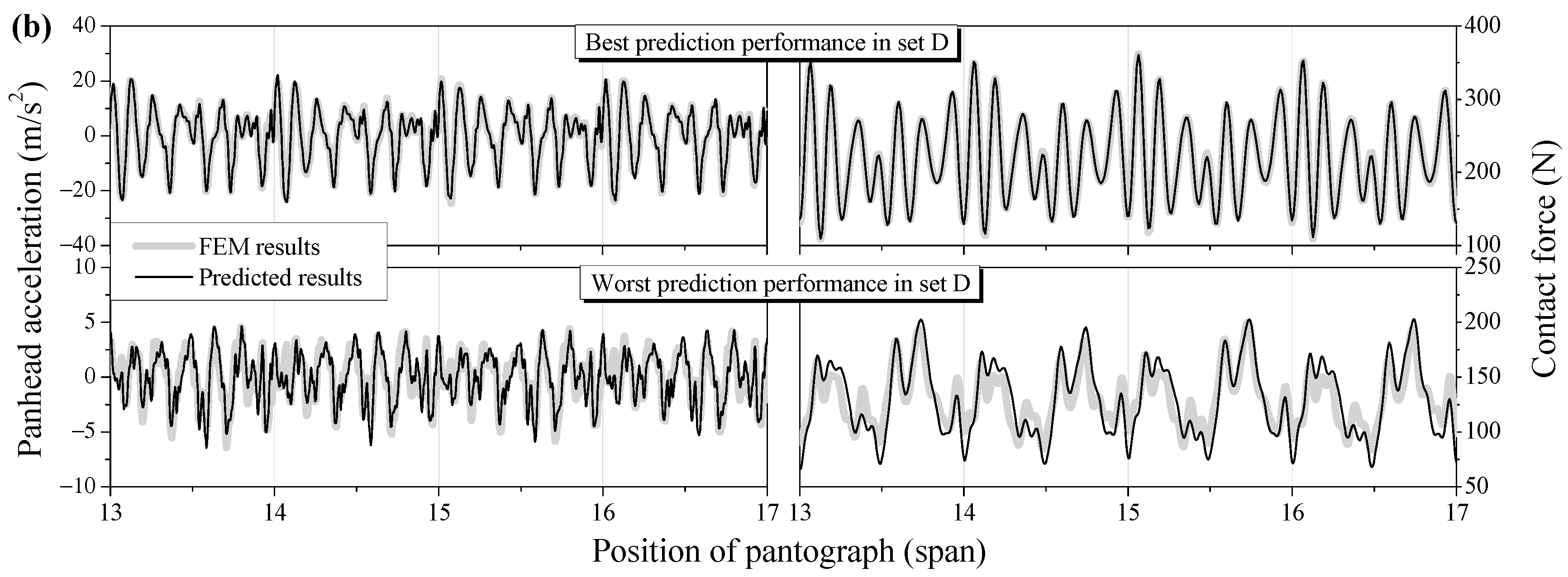
For set D with piecewise linear panhead stiffness, Figure 3b shows the time-domain signals of the panhead acceleration and the pantograph–catenary contact force of the samples with the best and worst prediction effect among them. Figure 4b shows the distribution of the determination coefficient of the time-domain signals and model errors of all samples. The relevant statistical values are given in the third row of Table 1. Similarly, the probability density of the determination coefficient between the model-predicted value and FEM-calculated value of the two kinds of time-domain signals presents a left-skewed distribution. The intervals within the probability of 0.95 of them are (92.5%, 100%> and (91.5%, 100%>, respectively, which means most of the values are greater than their mean values of 97.1% and 97.3%. For the sample with the maximum or the minimum determination coefficient, the model-predicted results of the two kinds of time-domain signals are in good agreement with their FEM results. In addition, the model-predicted values of the SDCF in these samples are basically the same as those of the FEM-calculated value (○ in Figure 5), and the determination coefficient between them is 98.2%. The probability density distribution of model errors is approximately symmetric, and the interval within the probability of 0.95 of the model errors is <−2.01, 4.11> N.
Therefore, the pantograph–catenary interaction prediction model demonstrates strong generalization ability. In addition, the prediction model required only 1 × 10⁻³ core hours, which is only 1/104 of the computational cost required for the FEM model in Section 2 when calculating a single pantograph–catenary interaction case.

4. Application in Optimization of Pantograph Parameters

At a specific running speed and low-pass filtering frequency, the optimal solution of the decision vector was achieved using SCSA with the objective of minimizing the SDCF. According to trade standards EN50318:2018 [23] and EN50317:2012 [29], the time-domain signal of contact force should be filtered through a 20 Hz low-pass filter. The analysis of the time-domain signals of contact force from the 4200 sets of FEM results involved above indicates that 95.45 ± 2.05% of the energy of the contact force signals is concentrated below 40 Hz. Therefore, two low-pass filtering frequencies, 20 and 40 Hz, were selected as the cut-off frequencies in the optimization. It is worth noting that the sampling frequency of the time-domain signal used in this paper is 200 Hz, which is five times higher than 40 Hz. According to the Nyquist–Shannon sampling theorem, such a sampling frequency is accurate enough to describe time-domain signals below 40 Hz. A total of nine speeds were selected with an interval of 25 km/h between 250 and 450 km/h; the decision vectors were set as X and Y, respectively, to study the effect of nonlinear stiffness panhead. The SDCF corresponding to the decision vector is given by the pantograph–catenary interaction prediction model. The value range of each decision variable in X and Y is the same as that in Section 3.3, and the maximum number of iterations is 200.
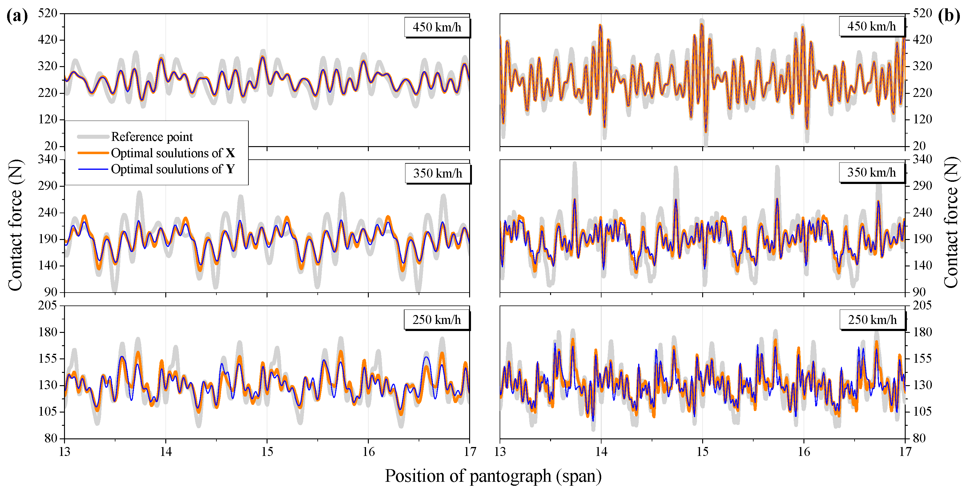
The time-domain signal of the contact force at the optimal solution and the reference point are shown in Figure 6, where the reference point represents the parameters of the existing DSA380 pantograph in service [7]. Compared with the reference point, the fluctuation degree of the time-domain signal at the optimal solution is significantly reduced, and the optimization effect varies at different speeds and low-pass filtering frequencies. In addition, under the same working condition, most of the peak-valley values of the time-domain signals are slightly lower in the case of nonlinear panhead stiffness compared to those in the case of linear panhead stiffness.
The decreased value of the SDCF of the optimal solution compared with the reference point Δσ was used as the quantitative index of the optimization effect. As the speed increases, the optimization effect tends to increase from about 5 N at medium speed to 18 N at higher speed (Figure 7a). However, the optimization effect has a local minimum at 375 km/h because the excitation frequency of the moving contact force at the nearby speed points, that is, 350 km/h and 400 km/h, is equal to the natural frequency of the catenary. This leads to the resonance of the pantograph and catenary, resulting in relatively high SDCF at 350 km/h and 400 km/h and relatively low SDCF at 375 km/h. Therefore, the optimization space at 375 km/h is relatively small, leading to the small size of Δσ. In addition, the optimization effect at 425 km/h and 450 km/h no longer increases with the increase in speed because the maximum natural frequency of the three-mass model of the pantograph is 17.7 Hz in the parameter value range, while the high-frequency components above 20 Hz of the contact force increase significantly when the running speed exceeds 400 km/h. This indicates that the joint optimization effect of pantograph parameters based on the three-mass model has limitations.
Furthermore, the influence of the low-pass filtering frequency and the panhead stiffness setting on the optimization effect are shown in Figure 7b. Whether the panhead stiffness is linear or nonlinear, the optimization effect of σ20 is slightly better than that of σ40 at medium and high speeds. But the difference is small, not more than 0.76 N. However, at higher speeds, due to the increase in high-frequency components of the contact force, the difference between the optimization effect of σ20 and that of σ40 increases to 1.23~5.44 N. The optimization effect of nonlinear panhead stiffness is slightly better than that of linear panhead stiffness, with the maximum difference being 2 N, occurring at 350 km/h.

5. Conclusions

In this paper, a data-physics coupling model that can quickly predict the pantograph–catenary interaction was proposed. In the process of obtaining the time-domain signal of the pantograph–catenary contact force, the time-consuming finite element solution process of the pantograph–catenary dynamic equation was avoided, and the time-domain signal of the panhead acceleration was taken as the boundary condition to directly solve the pantograph dynamic equation. The computational cost of this prediction model was only 1 × 10⁻³ core hours, which is only 1/104 of that of the traditional pantograph–catenary finite element model.
The application prospect of this model includes the following two aspects:
Firstly, whether in existing line tests or on the operational high-speed railway, compared with the real-time monitoring of the pantograph–catenary contact force, which requires changes in the panhead structure and installation of sensors, the non-contact test technology for panhead displacement is more mature and feasible. Based on the time-domain signal of panhead displacement, the time-domain signal of panhead acceleration can be obtained. Then, the time-domain signal of the contact force can be obtained using the pantograph–catenary interaction prediction model.
Secondly, for the multi-parameter joint optimization of the pantograph–catenary system, a greater number of decision variables leads to a more favorable optimization effect. However, the number of cases involved will increase sharply, and the computational cost required for the calculation based on the pantograph–catenary FEM model is extremely higher as the number of decision variables increases. In addition to greatly improving computational efficiency, the pantograph–catenary interaction prediction model can effectively predict the time-domain signal of the dynamic response of the pantograph–catenary system. In this paper, under different speeds, the prediction model was applied to the multi-parameter joint optimization of six pantograph dynamic parameters and nine pantograph dynamic parameters considering the nonlinear panhead stiffness. The optimization strategies outlined in this paper led to a significant 34.62% reduction in the SDCF. Based on all the working conditions concerned in this paper, it is suggested that m3 and m1 should be reduced to their lower limits; k3 should be increased, the increase depending on specific working conditions; m2 should be reduced at medium and higher speeds and increased at other speeds; k2 should be reduced to its lower limit at medium and high speeds, and increased at 375 km/h and above; and c1 should be reduced at medium speed and increased to its upper limit at the other speeds.

Author Contributions

Conceptualization, M.W. and X.X.; Methodology, M.W. and J.W.; Software, M.W.; Validation, H.Z. and R.Z.; Formal analysis, M.W., H.Z. and R.Z.; Investigation, M.W., H.Z. and R.Z.; Data Curation, M.W. and X.X.; Writing—Original Draft, M.W.; Writing—Review & Editing, X.X. and J.W.; Visualization, M.W. and X.X.; Supervision, X.X. and J.W.; Project administration, X.X. and J.W.; Funding acquisition, X.X. and J.W. All authors have read and agreed to the published version of the manuscript.

Funding

This work was supported by the Major Project of China Railway Co., Ltd., Beijing, China, (K2021J004-A) and the Strategic Priority Research Program of the Chinese Academy of Sciences (XDB22020201). The funder was not involved in the study design, collection, analysis, interpretation of data, the writing of this article or the decision to submit it for publication.

Institutional Review Board Statement

Not applicable.

Informed Consent Statement

Not applicable.

Data Availability Statement

The data presented in this study are available on request from the corresponding author. The data are not publicly available due to privacy.

Conflicts of Interest

The authors declare that this study received funding from the Major Project of China Railway Co., Ltd., Beijing, China, (K2021J004-A). The funder was not involved in the study design, collection, analysis, interpretation of data, the writing of this article or the decision to submit it for publication.

References

  1. Luo, W. Tech Upgrades Power Trains to 453 km/h during Tests. People’s Daily (Edition 2). 2 July 2023. Available online: http://paper.people.com.cn/rmrb/html/2023-07/02/nbs.D110000renmrb_02.htm (accessed on 3 July 2023).
  2. Poetsch, G.; Evans, J.; Meisinger, R.; Kortüm, W.; Baldauf, W.; Veitl, A.; Wallaschek, J. Pantograph/catenary dynamics and control. Veh. Syst. Dyn. 1997, 28, 159–195. [Google Scholar] [CrossRef]
  3. Bruni, S.; Ambrosio, J.; Carnicero, A.; Cho, Y.H.; Finner, L.; Ikeda, M.; Kwon, S.Y.; Massat, J.-P.; Stichel, S.; Tur, M.; et al. The results of the pantograph–catenary interaction benchmark. Veh. Syst. Dyn. 2015, 53, 412–435. [Google Scholar] [CrossRef]
  4. Bruni, S.; Bucca, G.; Carnevale, M.; Collina, A.; Facchinetti, A. Pantograph–catenary interaction: Recent achievements and future research challenges. Int. J. Rail. Transp. 2017, 6, 57–82. [Google Scholar] [CrossRef]
  5. Song, Y.; Antunes, P.; Pombo, J.; Liu, Z. A methodology to study high-speed pantograph-catenary interaction with realistic contact wire irregularities. Mech. Mach. Theory 2020, 152, 103940. [Google Scholar] [CrossRef]
  6. Cho, Y.H. Numerical simulation of the dynamic responses of railway overhead contact lines to a moving pantograph, considering a nonlinear dropper. J. Sound Vib. 2008, 315, 433–454. [Google Scholar] [CrossRef]
  7. Wu, M.; Xu, X.; Yan, Y.; Luo, Y.; Huang, S.; Wang, J. Multi-parameter joint optimization for double-strip high-speed pantographs to improve pantograph-catenary interaction quality. Acta Mech. Sin. 2022, 38, 521344. [Google Scholar] [CrossRef]
  8. Jimenez-Octavio, J.R.; Carnicero, A.; Sanchez-Rebollo, C.; Such, M. A moving mesh method to deal with cable structures subjected to moving loads and its application to the catenary–pantograph dynamic interaction. J. Sound Vib. 2015, 349, 216–229. [Google Scholar] [CrossRef]
  9. Gregoria, S.; Tur, M.; Nadala, E.; Aguado, J.V.; Fuenmayor, F.J.; Chinesta, F. Fast simulation of the pantograph-catenary dynamic interaction. Finite Elem. Anal. Des. 2017, 129, 1–13. [Google Scholar] [CrossRef]
  10. Gregori, S.; Tur, M.; Pedrosa, A.; Tarancón, J.E.; Fuenmayor, F.J. A modal coordinate catenary model for the real-time simulation of the pantograph-catenary dynamic interaction. Finite Elem. Anal. Des. 2019, 162, 1–12. [Google Scholar] [CrossRef]
  11. Wu, T.X.; Brennan, M.J. Basic Analytical Study of Pantograph-catenary System Dynamics. Veh. Syst. Dyn. 1998, 30, 443–456. [Google Scholar] [CrossRef]
  12. Lopez-Garcia, O.; Carnicero, A.; Marono, J.L. Influence of stiffness and contact modelling on catenary-pantograph system dynamics. J. Sound Vib. 2007, 299, 806–821. [Google Scholar] [CrossRef]
  13. Duan, H.Y.; Dixon, R.; Stewart, E. A disturbance observer based lumped-mass catenary model for active pantograph design and validation. Veh. Syst. Dyn. 2022, 61, 1565–1582. [Google Scholar] [CrossRef]
  14. Wu, T.X.; Brennan, M.J. Dynamic stiffness of a railway overhead wire system and its effect on pantograph–catenary system dynamics. J. Sound Vib. 1999, 219, 483–502. [Google Scholar] [CrossRef]
  15. Gil, J.; Gregori, S.; Tur, M.; Fuenmayor, F.J. Analytical model of the pantograph-catenary dynamic interaction and comparison with numerical simulations. Veh. Syst. Dyn. 2022, 60, 132–155. [Google Scholar] [CrossRef]
  16. Gil, J.; Tur, M.; Correcher, A.; Gregori, S.; Pedrosa, A.; Fuenmayor, F.J. Hardware-in-the-loop pantograph tests using analytical catenary models. Veh. Syst. Dyn. 2022, 60, 3504–3518. [Google Scholar] [CrossRef]
  17. Lee, J.-H.; Kim, Y.-G.; Paik, J.-S.; Park, T.-W. Performance evaluation and design optimization using differential evolutionary algorithm of the pantograph for the high-speed train. J. Mech. Sci. Technol. 2012, 26, 3253–3260. [Google Scholar] [CrossRef]
  18. Su, K.X.; Zhang, J.W.; Zhang, J.W.; Yan, T.; Mei, G. Optimisation of current collection quality of high-speed pantograph-catenary system using the combination of artificial neural network and genetic algorithm. Veh. Syst. Dyn. 2022, 61, 260–285. [Google Scholar] [CrossRef]
  19. Huang, G.Z.; Wu, G.N.; Yang, Z.F.; Chen, X.; Wei, W. Development of surrogate models for evaluating energy transfer quality of high-speed railway pantograph-catenary system using physics-based model and machine learning. Appl. Energy 2023, 333, 120608. [Google Scholar] [CrossRef]
  20. Song, Y.; Wang, H.R.; Frøseth, G.; Nåvik, P.; Liu, Z.; Rønnquist, A. Surrogate modelling of railway pantograph-catenary interaction using deep Long-Short-Term-Memory neural networks. Mech. Mach. Theory 2023, 187, 105386. [Google Scholar] [CrossRef]
  21. Zhou, R.; Xu, X.H. Dynamic parameter optimization of high-speed pantograph base on swarm intelligence and machine learning. Int. J. Appl. Mech. 2023, 15, 2350078. [Google Scholar] [CrossRef]
  22. Wu, M.Z.; Liu, Y.; Xu, X.H. Sensitivity analysis and optimization parameters of high speed pantograph-catenary system. Chin. J. Theor. Appl. Mech. 2021, 53, 75–83. [Google Scholar] [CrossRef]
  23. EN50318:2018; Railway Applications-Current Collection Systems-Validation of Simulation of the Dynamic Interaction between Pantograph and Overhead Contact Line. European Committee for Electrotechnical Standardization: Brussels, Belgium, 2018.
  24. Mckay, M.D.; Conover, R.J.B.J. A comparison of three methods for selecting values of input variables in the analysis of output from a computer code. Technometrics 1979, 21, 239–245. [Google Scholar]
  25. Broomhead, D.S.; Lowe, D. Radial Basis Functions, Multi-Variable Functional Interpolation and Adaptive Networks; Royal Signals and Radar Establishment: Malvern, UK, 1988. [Google Scholar]
  26. Jebari, K.; Madiafi, M. Selection Methods for Genetic Algorithms. Int. J. Emerg. 2013, 3, 333–344. [Google Scholar]
  27. Askarzadeh, A. A novel metaheuristic method for solving constrained engineering optimization problems: Crow search algorithm. Comput. Struct. 2016, 169, 1–12. [Google Scholar] [CrossRef]
  28. EN50367:2020; Railway Applications-Current Collection Systems-Technical Criteria for the Interaction between Pantograph and Overhead Line. European Committee for Electrotechnical Standardization: Brussels, Belgium, 2020.
  29. EN50317:2012; Railway Applications-Current Collection Systems-Requirements for and Validation of Measurements of the Dynamic Interaction between Pantograph and Overhead Contact Line. European Committee for Electrotechnical Standardization: Brussels, Belgium, 2012.
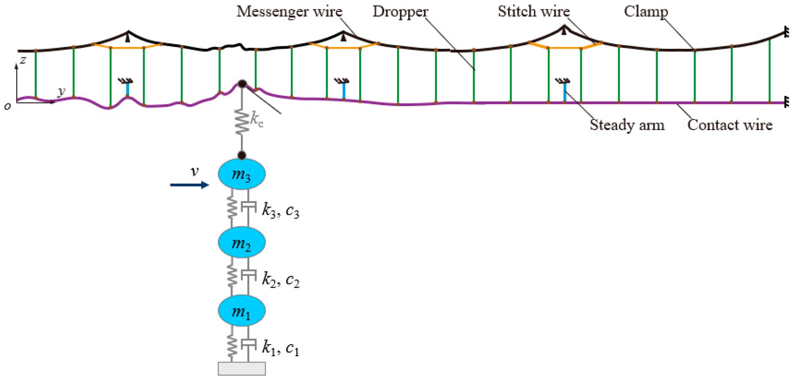
Figure 1. Pantograph–catenary finite element model.
Applsci 14 00449 g001
Figure 2. Pantograph–catenary interaction prediction model.
Applsci 14 00449 g002
Figure 3. Model predicted time-domain signals in test sets C (a) and D (b).
Applsci 14 00449 g003aApplsci 14 00449 g003b
Figure 4. Distribution of determination coefficients of time-domain signals and model errors: (a) set C; (b) set D.
Applsci 14 00449 g004
Figure 5. σ q and σ ^ q of test set samples.
Applsci 14 00449 g005
Figure 6. Time-domain signal of contact force with low-pass filtering frequency of 20 Hz (a) and 40 Hz (b).
Applsci 14 00449 g006
Figure 7. Optimization effect (a) and its influencing factors (b).
Applsci 14 00449 g007
Table 1. Generalization ability of pantograph–catenary interaction prediction model.
Test SetDetermination Coefficient (%)Model Error (N)
z ¨ 3 t F c t σInterval within Probability of 0.95
Mean Value Interval within Probability of 0.95Mean Value Interval within Probability of 0.95
C97.7(92.8, 100>97.4(91.0, 100>98.2<−2.35, 3.60>
D97.1(92.5, 100>97.3(91.5, 100>98.2<2.01, 4.11>
Disclaimer/Publisher’s Note: The statements, opinions and data contained in all publications are solely those of the individual author(s) and contributor(s) and not of MDPI and/or the editor(s). MDPI and/or the editor(s) disclaim responsibility for any injury to people or property resulting from any ideas, methods, instructions or products referred to in the content.