Abstract
The steel industry is typical process manufacturing, and the quality and cost of the products can be improved by efficient operation of equipment. This paper proposes an efficient diagnosis and monitoring method for the gearbox, which is a key piece of mechanical equipment in steel manufacturing. In particular, an equipment maintenance plan for stable operation is essential. Therefore, equipment monitoring and diagnosis to prevent unplanned plant shutdowns are important to operate the equipment efficiently and economically. Most plant data collected on-site have no precise information about equipment malfunctions. Therefore, it is difficult to directly apply supervised learning algorithms to diagnose and monitor the equipment with the operational data collected. The purpose of this paper is to propose a pseudo-label method to enable supervised learning for equipment data without labels. Pseudo-normal (PN) and pseudo-abnormal (PA) vibration datasets are defined and labeled to apply classification analysis algorithms to unlabeled equipment data. To find an anomalous state in the equipment based on vibration data, the initial PN vibration dataset is compared with a PA vibration dataset collected over time, and the equipment is monitored for potential failure. Continuous wavelet transform (CWT) is applied to the vibration signals collected to obtain an image dataset, which is then entered into a convolutional neural network (an image classifier) to determine classification accuracy and detect equipment abnormalities. As a result of Steps 1 to 4, abnormal signals have already been detected in the dataset, and alarms and warnings have already been generated. The classification accuracy was over 0.95 at , confirming quantitatively that the status of the equipment had changed significantly. In this way, a catastrophic failure can be avoided by performing a detailed equipment inspection in advance. Lastly, a catastrophic failure occurred in Step 9, and the classification accuracy ranged from 0.95 to 1.0. It was possible to prevent secondary equipment damage, such as motors connected to gearboxes, by identifying catastrophic failures promptly. This case study shows that the proposed procedure gives good results in detecting operation abnormalities of key unit equipment. In the conclusion, further promising topics are discussed.
1. Introduction
In the steel industry, which is representative of process manufacturing, 10% to 20% of production costs are spent on equipment maintenance. Operation of key machines efficiently and economically is an important issue to gain an edge in quality and cost competitiveness, which are directly related to corporate survival [1,2]. If an unplanned plant shutdown occurs in steel production equipment, not only will there be significant economic loss, but it will also have a negative impact on product quality, so it is important to detect equipment abnormalities quickly and handle the problem proactively before catastrophic breakdowns occur. It is known that maintenance in response to unplanned failures is three to nine times the cost of predictive maintenance. According to statistics from the United States Department of Commerce (2003), which investigated industrial economic costs due to unplanned production interruptions, the annual cost of equipment maintenance in US industry amounted to $4.9 trillion as of 2003. The Federal Energy Management Program (FEMP) reported that 8% to 12% of costs can be saved through predictive maintenance compared to preventive maintenance. The effects of predictive maintenance can be expected to reduce equipment maintenance costs, prevent unplanned plant downtime, and improve productivity and quality. As a result of analyzing failures that occurred at one steel company, 65% of them were considered preventable through inspection and monitoring, and only 35% were found to require break-down maintenance.
A gearbox is an important mechanical equipment that transmits power between shafts. Among single-equipment failures, gearbox-related failures were found to be the highest at 38% in one steel company. As the types of steel produced become more diverse, machines operate at higher loads than that for which they were designed. A sudden failure of a gearbox can cause quality defects, expensive repairs, and even accidents. The health of a gearbox can be confirmed by measuring machine vibrations, acoustics, heat, and iron content in lubricants. Among these, vibration signals are the most widely used because they contain much information from inside mechanical equipment [3]. Vibration signals measured in all mechanical devices have a specific spectrum when operating normally, but the spectrum changes when failure occurs, so vibration signals are the most effective way to monitor and diagnose the health of rotating mechanical equipment. However, one problem is that extracting features from vibration signals related to gearbox or bearing failures requires extensive domain expertise and prior empirical knowledge. Recently, the rapid development of artificial intelligence (AI) is accelerating developments in the field of intelligent fault diagnosis, along with research on effective and highly accurate fault detection methods that do not rely on feature extraction [4,5].
Research has continued in the field of anomaly detection, but supervised learning algorithms, such as classification, regression, and object identification, have been proposed more frequently than unsupervised learning algorithms. Additionally, supervised learning provides various evaluation indicators such as accuracy, precision, and recall. Field vibration data are collected over time without a label indicating whether it is normal or abnormal. As a result, unsupervised learning methods are required due to limitations.
In the case of steel manufacturing equipment, many data are collected in real time from vibration and temperature sensors, but since there are many customary events, such as overhauls, minor repairs, and oil replacement, it is difficult to define in advance a label that indicates whether the equipment state is normal or not. Therefore, time series data are collected without prior information on the occurrence of failures, which cannot be used in a classification model to detect machine abnormalities [6,7]. In this paper, we propose the application of a pseudo-label method for collecting gearbox vibration signals without labels that indicate whether the equipment has failed. Through modeling and analysis of data collected from steel manufacturing equipment, we show that classification analysis with pseudo-labels can provide alarm and warning for equipment abnormalities.
The rest of the paper is organized as follows: Section 2 covers related studies and issues. Section 3 presents a pseudo-labeling(proposed) method and a procedure for monitoring equipment status changes. Section 4 describes the theoretical background of CWT, CNN, and evaluation metrics. In Section 5, data acquisition and pre-processing are covered, and the CNN classifier is designed. Finally, Section 6 summarizes the experimental results and conclusion.
2. Related Works
According to existing research, supervised learning techniques are used 88% of the time when analyzing equipment failure data, and unsupervised learning techniques 12% of the time [8]. When using supervised learning, a fault identification study is performed under the assumption that data are collected with labels indicating the presence or absence of faults. When using unsupervised learning, research is conducted for anomaly detection. With unlabeled data, statistical methods such as regression analysis, time series analysis, and probabilistic models are studied to detect anomalies and construct a regression model to analyze abnormal conditions on ships and the changes detected [9].
When computer scientist Geoffery Hiton began researching deep learning in 2010, it began replacing methods like regression models, support vector machines (SVM), and decision trees (DT), which were widely used as existing machine learning methods. The main reason for the rapid spread of deep learning is its high performance and ease of problem-solving by automating feature engineering (the most important step in machine learning). In machine learning, developers must create good features from the data, whereas deep learning simplifies the application of machine learning by learning all features at once. Research on monitoring and diagnosing equipment problems by utilizing these features of deep learning is underway. We will be examining related research on equipment abnormality detection using CNN after confirming the application cases of autoencoder, a deep learning method that is unsupervised [10,11,12]. We will be examining the latest research trends combining LSTMs with autoencoders, both of which are specialized for the analysis of time series data [13,14,15]. Perera and Brage [16] proposed a method of classifying data using the expectation-maximization technique and a Gaussian mixture model (GMM) and then monitoring performance using an autoencoder (AE, an unsupervised learning algorithm). The autoencoder is an unsupervised learning technique that uses neural networks to learn representations. When input comes in, the neural network compresses it as much as possible, extracts the characteristics of the data, and restores it to its original form. Anomaly detection is one of many applications of AE beyond its general use in dimension reduction. Jeong [17] applied a convolutional artificial neural network to diagnose the state of a rotating body in advance and used orbit analysis to diagnose the condition of the rotating body. The orbit represents the dynamics of the rotating body and visually expresses the state of the equipment. Additionally, the orbit shape is converted into an image, and the image pattern is used as input data for the convolutional artificial neural network. Jung [18] studied failure diagnosis for journal-bearing rotor systems using a convolutional artificial neural network. They applied an omnidirectional regenerator (ODR) technique based on the vibration data acquired to obtain signals in the circumferential direction, used them to generate a vibration signal-based image and then used the image as input to a convolutional artificial neural network. Gao et al. [19] conducted a study to diagnose roller bearing abnormalities using continuous wavelet transform and a convolutional artificial neural network. They propose image recognition based on time-frequency diagrams and Convolution Neural Networks (CNN). First, joint time-frequency analysis (JTFA) using continuous wavelet transform (CWT) of complex Morlet wavelet is used to obtain the time-frequency diagram characteristics of the vibration signal and normalize it to obtain the input of CNN. JTFA converts one-dimensional time domain signals into a two-dimensional representation of energy versus time and frequency. There are several different transforms available in the JTFA. A different time-frequency representation is shown for each transform type. Short-Time Fourier Transforms (STFT) are the simplest JTFA transformations. The CNN is then trained with labeled time-frequency diagrams. Finally, the trained model is used to diagnose defect types in the unknown data. The effectiveness of the proposed method was verified through fault simulation experiments.
The autoencoder LSTM detected gear faults using time series data, and Lee et al. [20] used it to detect abnormalities in his data. LSTMs are designed to solve the long-term dependencies of RNNs. Hence, this model is designed to predict future data by combining not only the past data but also the past data in its broader sense. Using an empirical wavelet transform based on the Fourie-Bessel domain, Ramteke et al. [21] proposed an automated classification framework for diagnosing gear failures.
Steel manufacturing sites conduct equipment vibration and temperature data collection and analysis with a condition monitoring system (CMS). The vibration signal measured is converted to an average value in seconds or minutes and is then compared to a preset threshold to generate a two-stage alarm (alarm and warning). However, field mechanics do not have a high level of trust in the CMS; false alarms frequently occur because the CMS does not reflect sensor noise, shock vibration due to the surrounding environment, vibration changes depending on operating conditions, and equipment repair history. The main reasons for frequent false alarms are that the CMS does not reflect event data such as oil changes, overhauls, and minor repairs and does not take into account equipment operation conditions with fluctuating loads. Many equipment abnormality monitoring and diagnostic studies are conducted based on classification algorithms, and this is due to the clarity of evaluation and the diversity in classification algorithms. In this paper, to practically use the advantages of a classification algorithm, we show that it is possible to monitor and diagnose equipment abnormalities by assigning pseudo-labels to unlabeled time series data and designing a classifier [22,23,24,25].
3. A Monitoring Procedure for Equipment Status
3.1. Methods for Capturing Changes in Equipment Status
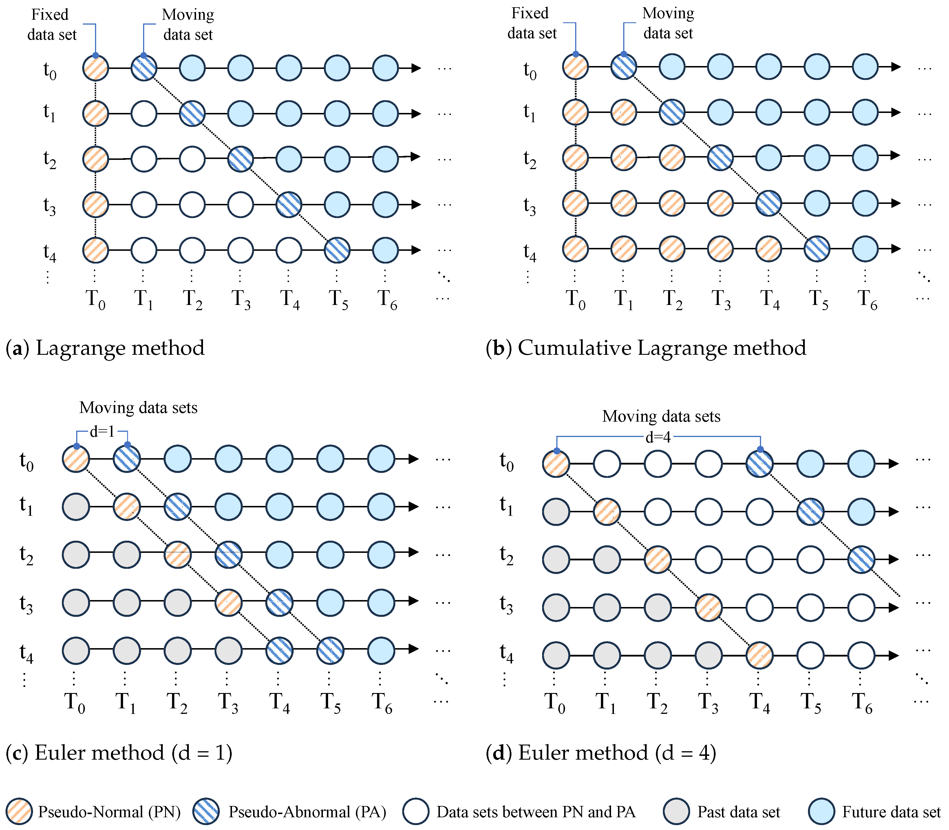
In this paper, we propose an approach to capturing anomalous equipment vibrations via signals obtained from a motor-gearbox test rig configured like field equipment. One technique for capturing the movement of particles in fluid mechanics is the Lagrangian perspective. As shown in Figure 1a,b, the Lagrange method is explained. Lagrange labeled the dataset at time by fixing it to pseudo-normal in Figure 1a. Pseudo-Abnormal labels the dataset at , which is the next data stamp, and divides it into training and test datasets. Using the prepared data, apply the classification algorithm and save the classification results. As a next step, the dataset at will be set as PN, whereas the dataset at will be labeled as a new PA. In order to apply the classification algorithm, all the previous steps must be repeated. If we can be sure that the standard dataset contains normal data, we can use the Lagrangian method to know when the state changes from normal to abnormal. Figure 1b shows a Cumulative Lagrange method that aggregates PA datasets into PN datasets using the classification algorithm. In Figure 1c,d, the Euler method is explained. In contrast to the Lagrange method, the Euler method moves the PN dataset according to the classification sequence while maintaining a certain interval (d) from the PA dataset. The Euler perspective labels datasets with certain specific distances for PN and PA datasets, so it has the advantage of being able to detect changes in equipment status more sensitively than the Lagrangian perspective. If a classification algorithm can be applied to the two labeled datasets, and if the classification performance is excellent, we can know that a significant change has occurred between the two datasets. The ideas about the Lagrange and Euler perspective are similar to the methods analyzing the flow field in fluid mechanics (Philip et al. [26]).
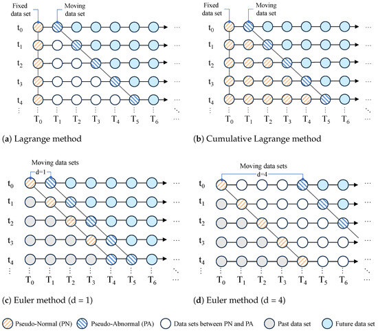
Figure 1.
Proposed Pseudo-Labeling method; : Data time stamp, : Classification sequence.
3.2. Monitoring for Equipment Abnormality
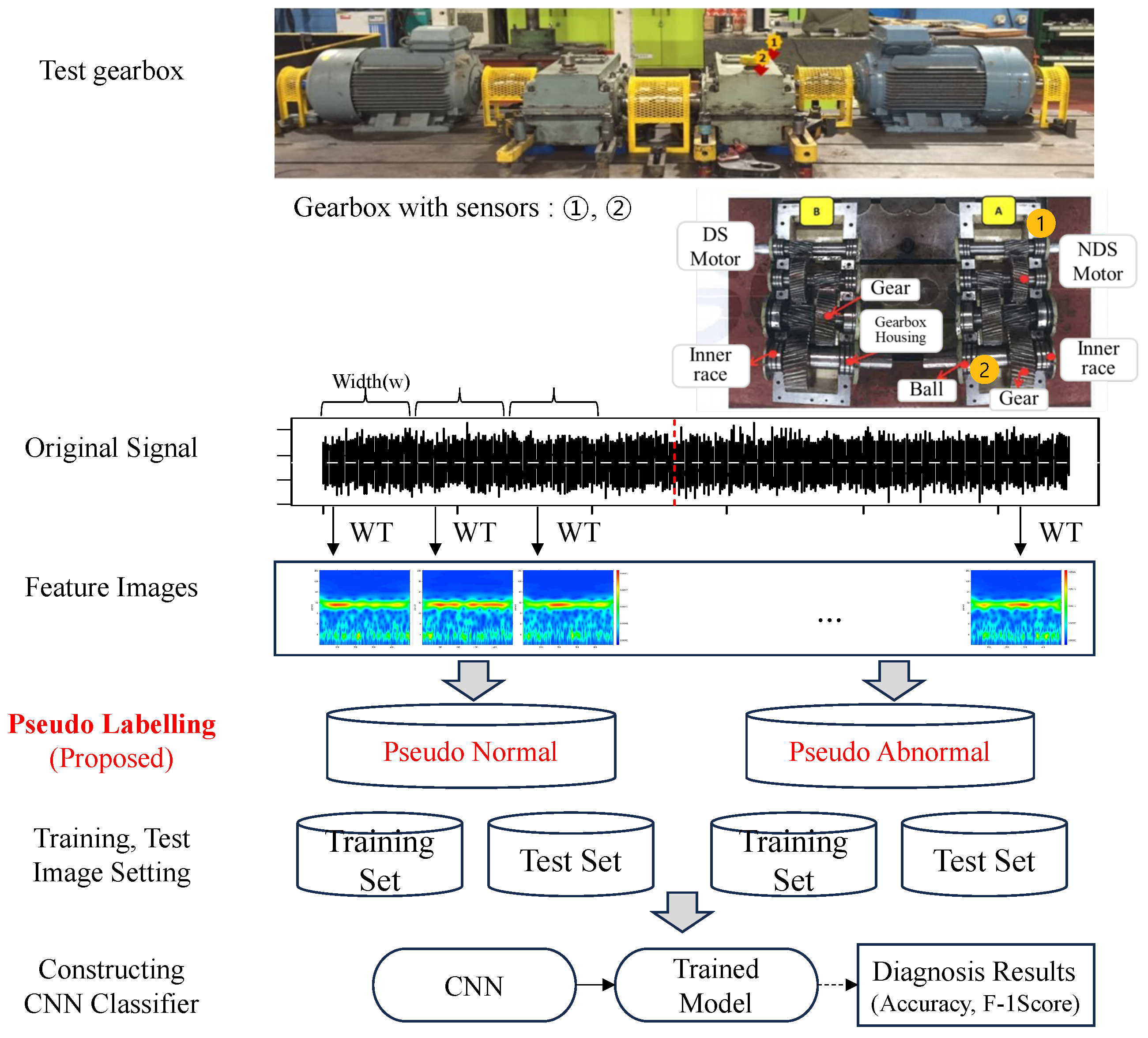
In this paper, we propose a procedure for monitoring and diagnosing changes in equipment status using a supervised learning algorithm that collects vibration data from unlabeled gearboxes, as shown in Figure 2. First, we select an appropriate window size (w) for equipment vibration data collection to monitor equipment status and extract images using continuous wavelet transform (CWT). The image dataset does not yet have teaching labels for normal and abnormal states, so a supervised learning algorithm cannot be used. Using the Euler method, the data are divided into PN and PA datasets. The interval parameter required in the Euler method is related to the latency period of equipment faults and is monitored when interval parameter and . After assigning pseudo-labels and configuring training and test datasets, it is possible to obtain accuracy and image classification performance measures using the CNN image classifier. If the classification performance metric(, , , ) is above 0.80, it generally means there is a significant difference between the two datasets.
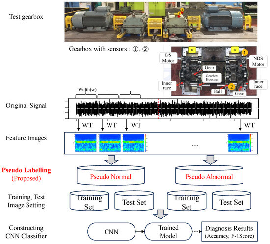
Figure 2.
Flowchart of the proposed procedure (1, 2: Sensor positions/A: Non drive side, B: Drive side).
4. Theoretical Background
4.1. Continuous Wavelet Transform
In this section, we briefly review continuous wavelet transformation (CWT), which is a method of analyzing the time and frequency domains simultaneously via wavelet transform. Wavelet transform (WT) is a method of decomposing arbitrary signals into functions defined as wavelets. When a signal obtained from equipment is subjected to CWT, time and frequency characteristics are generated as an image; for detecting equipment abnormalities, images are used to feed convolutional neural networks [27,28,29,30]. The wavelet function, , can be obtained by scaling and translating the parent wavelet function as shown in Equation (1):
where a is a scale parameter related to the time resolution of the wavelet function, b is a translation parameter that determines the position of the wavelet function on the time axis, and represents the mother wavelet. The wavelet transform is the inner product between the given function and the wavelet function, as shown in Equation (2). For any signal function given, can be integrated over the entire interval, and the CWT is defined mathematically as follows:
Here, is the complex conjugate function of the mother wavelet function . Based on the above operation, signal is transformed and projected into two dimensions (time and scale), and the one-dimensional time series is converted into a two-dimensional time-frequency image. The choice of the mother wavelet function influences classification accuracy significantly. Depending on the mother wavelet, there are pros and cons. In continuous wavelet transform, Bump, Mexican hat, Morlet, Paul mother wavelet, etc., are commonly used. Mexican hat and Paul mother wavelets are known for their advantages in time domain analysis. The Morlet mother wavelet, however, has advantages in frequency analysis. The bump wavelet has a band shape and is suitable for analyzing frequencies locally. In this paper, Molet wavelets were used to analyze gearbox vibration data, which has the advantage of extracting features in the frequency domain that are difficult to identify in the time domain. The Morlet wavelet function is
4.2. Convolutional Neural Networks
Unlike the feature extraction step in the existing data-based analysis, deep learning techniques can learn optimal hierarchical features directly from the data and show high-quality performance in fields such as voice and object recognition. The convolutional artificial neural network can be viewed as an integrated model that combines the two steps of feature extraction and classification in existing pattern recognition methods into one step and is basically composed of multiple convolution layers and subsampling layers. A convolutional artificial neural network consists of a convolution layer, a pooling layer, and a fully connected (FC) layer. After the input layer, the convolution and pooling layers are repeated, and the last one or two layers include a fully connected layer. Many feature maps can be generated by convoluting input images with multiple convolution kernels on the convolution layer, and their results are input into the activation function as follows:
where represents the th element of the th layer, represents the th convolution region of the th layer, represents the element, is the weight matrix, represents bias, and is the activation function. A rectified linear unit (ReLU) is the most popular activation function and is given by
Pooling layers often follow convolution layers to realize the dimension reduction of feature maps and to keep the invariance of characteristic scales. The most commonly used pooling approaches are maxpooling, mean pooling, and stochastic pooling. In general, pooling layers are used only to implement a decrease of dimension without updating weights. After input images are alternately propagated by convolution and pooling steps, the extracted information and features are classified using the fully connected layer net. On FC layers, the input data are weighted summations of 1-D feature vectors:
where n is the sequence number of net layers, is the output of the fully connected layer, is the 1-D feature vectors, is a weight coefficient, and represents biases. The commonly used activation function is SoftMax.
4.3. Overview of Model Performance Evaluation Metrics
To properly estimate their capabilities, it is crucial to thoroughly examine the diagnostic abilities of several machine learning algorithms while accounting for variables such as model complexity, computational needs, and parameterization. For this reason, it is necessary to use defined criteria for assessing performance and discriminating between candidates. , , , , and false alarm rates are among these parameters. With these measurements, we can objectively compare and assess the performance of various models, allowing us to make informed decisions based on their individual benefits and drawbacks [27,28]. These are some of the evaluation metrics that have been used in studies; see Equations (7)–(10).
True Positive () indicates that the model predicted a true outcome, and the observation was accurate. False Positive () indicates that the model predicted a true result, but the actual result was false. False Negative () indicates a model that predicted a false result while the actual result was accurate. True Negative () indicates that the model predicted a false outcome, and the actual outcome was also false. The accuracy of a model is often used to evaluate its performance; however, the accuracy has several drawbacks as well. In unbalanced datasets, one class is more common than the other, and the model labels observations based on this imbalance. In the case of 90% false cases and only 10% true cases, there is a very high possibility that our model would have an accuracy score around 90%. Precision is calculated as the number of true positives over the total number of positives predicted by your model. This metric allows you to calculate the rate at which your positive predictions actually come true. The sensitivity (also known as recall) is the percentage of actual positive outcomes over your true positives. It is possible to evaluate how well our model predicts the true outcome. The is the harmonic mean of precision and recall. It can be used as an overall metric that incorporates both precision and recall. We use the harmonic mean instead of the regular mean because the harmonic mean punishes values that are far apart. This paper evaluated classification performance using accuracy, precision, and using a confusion matrix. There are deviations in individual values for each classification performance evaluation, but the overall trend is similar. Accuracy has less deviation than other indicators and stable values.
5. Experiment Validation
5.1. Data Acquisition and Pre-Processing
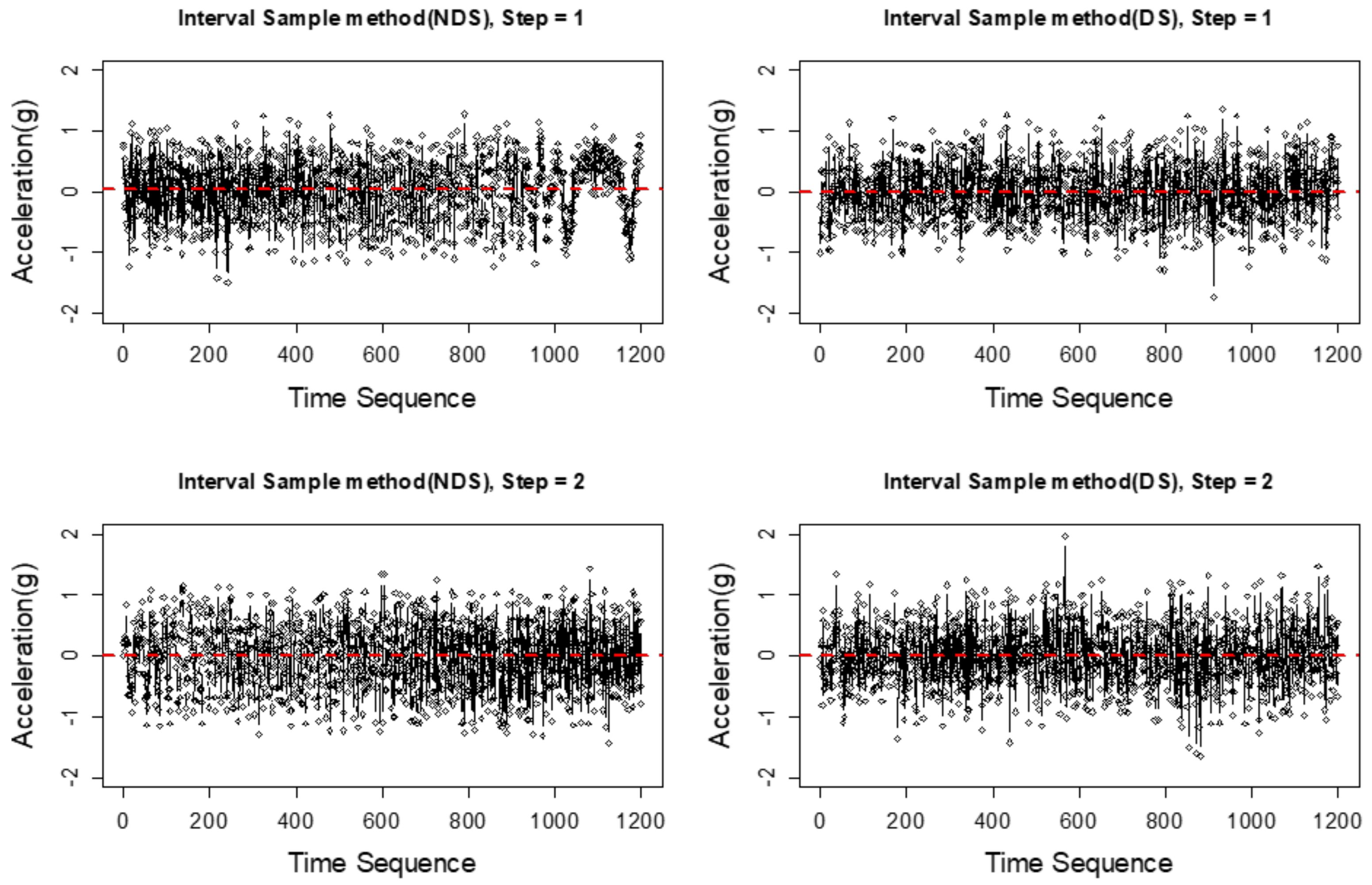
To monitor for abnormal conditions in gearboxes, vibration measurement sensors were attached to the drive side (DS) and non-drive side (NDS), as shown in Figure 2. The sensor specifications are as follows: Sensitivity (±10%) 100 mV/g, Setting Time <2.5 s, Spectral Noise at 10 Hz 14 g/Hz; Spectral Noise at 100 Hz 2.3 g/Hz Data for Sampling Speed was collected at s, but it was converted to s before pre-processing. We extracted one image for every 500 ea of pre-processed vibration data (window size = 500). To monitor equipment abnormalities, the gear teeth were arbitrarily damaged, and the operation was started, ultimately reaching a catastrophic failure in which the gear teeth were destroyed. Data were collected from both the DS and the NDS through acceleration and vibration sensors. The experimental device consisted of a 37 kW six-pole motor and four gears (a reduction ratio of and torque of up to 297 N·m). The collected continuous data included vibration data with time series characteristics in units of gravitational acceleration: g (m/s). Data were collected with synchronized time stamps and stored in a database. Source data were collected every s and stored every s because of computation power. We aggregated 500 pieces of data into one bundle and defined the window size (w) for analysis. Some original vibration data from the gearbox have been captured. Some of the original vibration data of the gearbox are shown in Figure 3. The original dataset, 46 ea files, is divided into 10 equal parts, resulting in 10 steps. A step divides the data into 10 sections, and each section contains 27,600 images in Figure 4. A gearbox was damaged by missing gear teeth, and alarm and warning signals were obtained through the proposed method in advance.
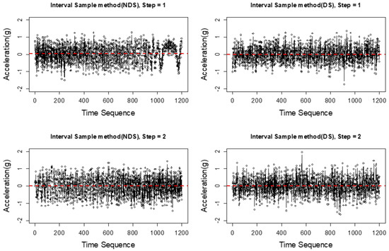
Figure 3.
DS and NDS gearbox vibration signal examples; step = 1, 2.
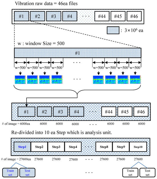
Figure 4.
Dataset preparation process for data analysis (Step1–10).
5.2. Image Extraction and CNN Design
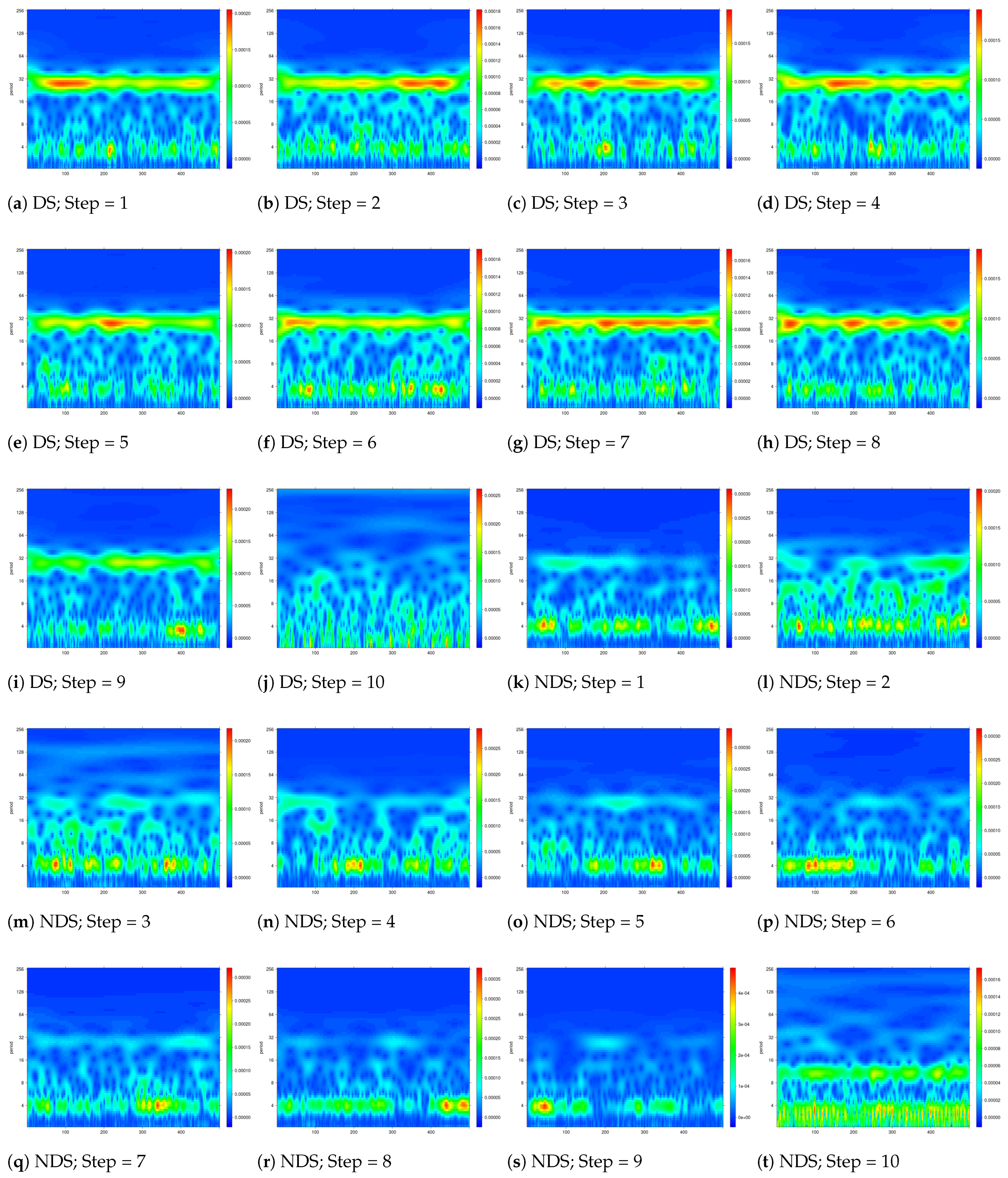
The source data were stored and divided for each rotation cycle, with time placed on the horizontal axis, period on the vertical axis, and RGB (red/green/blue) used for frequency intensity through continuous wavelet transformation. Data were converted into expressed images (Figure 5). In other words, instead of going through the feature extraction and selection steps from the equipment data to monitor changes in equipment status, a continuous wavelet transformation step and an input image preparation step were performed to visualize the vibration data. Since a converted image does not have a label indicating the presence or absence of abnormality, a direct classification algorithm cannot be used. Thus, the equipment status change capture method proposed in this paper was used. Through this, pseudo-labels are assigned, and images are classified using a convolutional artificial neural network. The collected vibration signals were divided at regular intervals (w), and the data were used to create a feature image set through CWT. At this time, the feature image set was labeled PN and PA at a 7:3 ratio and stored using the Eulerian perspective method. After dividing those data into training feature image sets, and testing feature image sets with pseudo-labels, they were labeled pseudo-normal and pseudo-abnormal at a 7:3 ratio and stored. A feature image with a pseudo-label was trained with the CNN and used as a classifier. The structure and number of main parameters of the CNN designed [31] in this paper are shown in Figure 6 and Table 1.
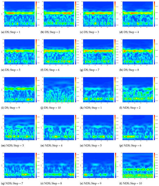
Figure 5.
Feature image example converted using continuous wavelet transform; DS and NDS, Step = 1, 2, 3, 4, 5, 6, 7, 8, 9.

Figure 6.
Convolutional Neural Network Structure.

Table 1.
Layer, output shape, and parameters of the convolutional neural network.
5.2.1. Convolution Layer
Input image data are expressed as a 3-dimensional tensor with height, width, and channel, and channel size is 3. In the first convolution layer, the filter size was 6 × 6, and in the second layer, the filter size was 4 × 4. It was designed to keep computation time constant at each layer. With the sigmoid function, learning becomes more difficult as neural network depth increases, but the ReLU function solves this problem. There is no vanishing gradient phenomenon in the ReLU function. With the sigmoid function as an activation function, the output value ranges between 0 and 1, so the vanishing gradient phenomenon occurs. The second advantage is that it is faster than existing activation functions (sigmoid, hyper-tangent). Thirdly, saturation problems can be avoided. The fourth advantage of ReLU is that it produces sparse activation. In general, the implementation is simple, the computational cost is low, and the performance is good.
5.2.2. Pooling Layer
As the number of computations increases exponentially with a fully connected layer, over-fitting problems may occur. A pooling layer is used to solve this problem. To adjust the image to an appropriate size and emphasize specific features, we selected a 3 × 3 pooling layer and a 2 × 2 pooling layer. After passing through the 2 × 2 pooling layer, the output is reduced by 1/4. As a result of Max Pooling, neurons respond to the largest signals, therefore reducing noise, increasing speed, and improving image discrimination.
5.2.3. Dropout Layer
To solve over-fitting, a dropout layer is added to the model. Different dropout rates were used for each dropout layer. Because there is a possibility of over-fitting in the case of the dropout_4 layer with many parameters, the dropout ratio was designed to be high at 50%, and the dropout_5 layer was designed at 20%. This method prevents over-fitting by disabling some hidden layer units randomly selected at random.
5.2.4. Fully Connected Layer Layer
For the fully connected layer, the SoftMax layer unit 2 was used to perform the classification of two values.
5.2.5. Regulation of Over-Fitting
An effective and widely used regularization technique to regulate over-fitting is adding a dropout layer. Because dropout reduces interdependence between neurons, it reduces over-fitting. Consequently, the neural network is unable to learn from all neurons, reducing its ability to remember information and generalize it. All the data were divided and trained, rather than all being put in at once. We use the concepts of batch size, epoch, and iteration at this time. In one epoch, learning is completed once for all datasets. This study used epoch 10 as the epoch. We considered that over-fitting could occur if the epoch is too large, and under-fitting could occur if the epoch is too small. As training and test data, 270 images were used, and the batch size, which refers to the number of images given per batch, was 15. The training data were randomly shuffled every epoch when the shuffle option was set to True. The test target image was used as validation data when learning the model.
5.3. Experiment Results
In this section, we apply the Euler method in which the interval between PN and PA is very important for efficiently detecting changes in equipment status. A change point is a point where the mean and variance of classification accuracy change, which indicates that a change has occurred in the data. The change point can be quantitatively determined through change point analysis. It is possible, however, that the change point represents the beginning of equipment damage, but further analysis is needed to confirm this.
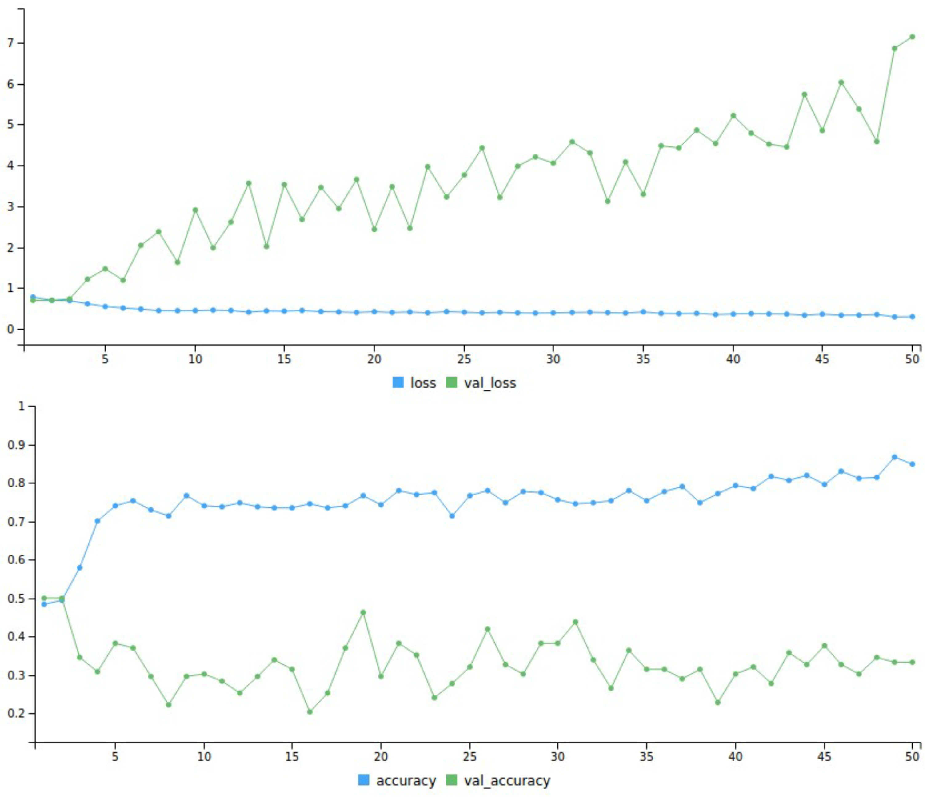
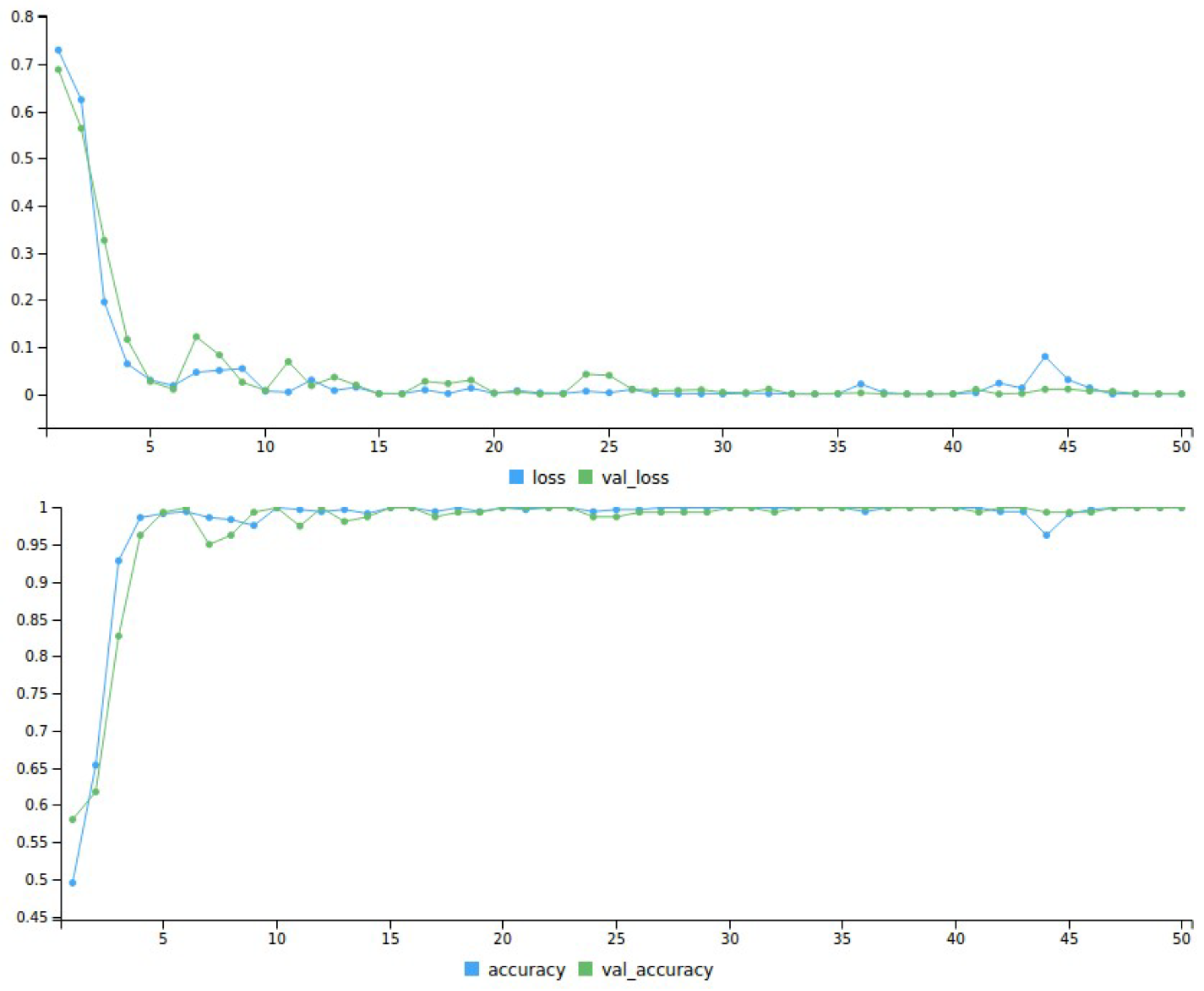
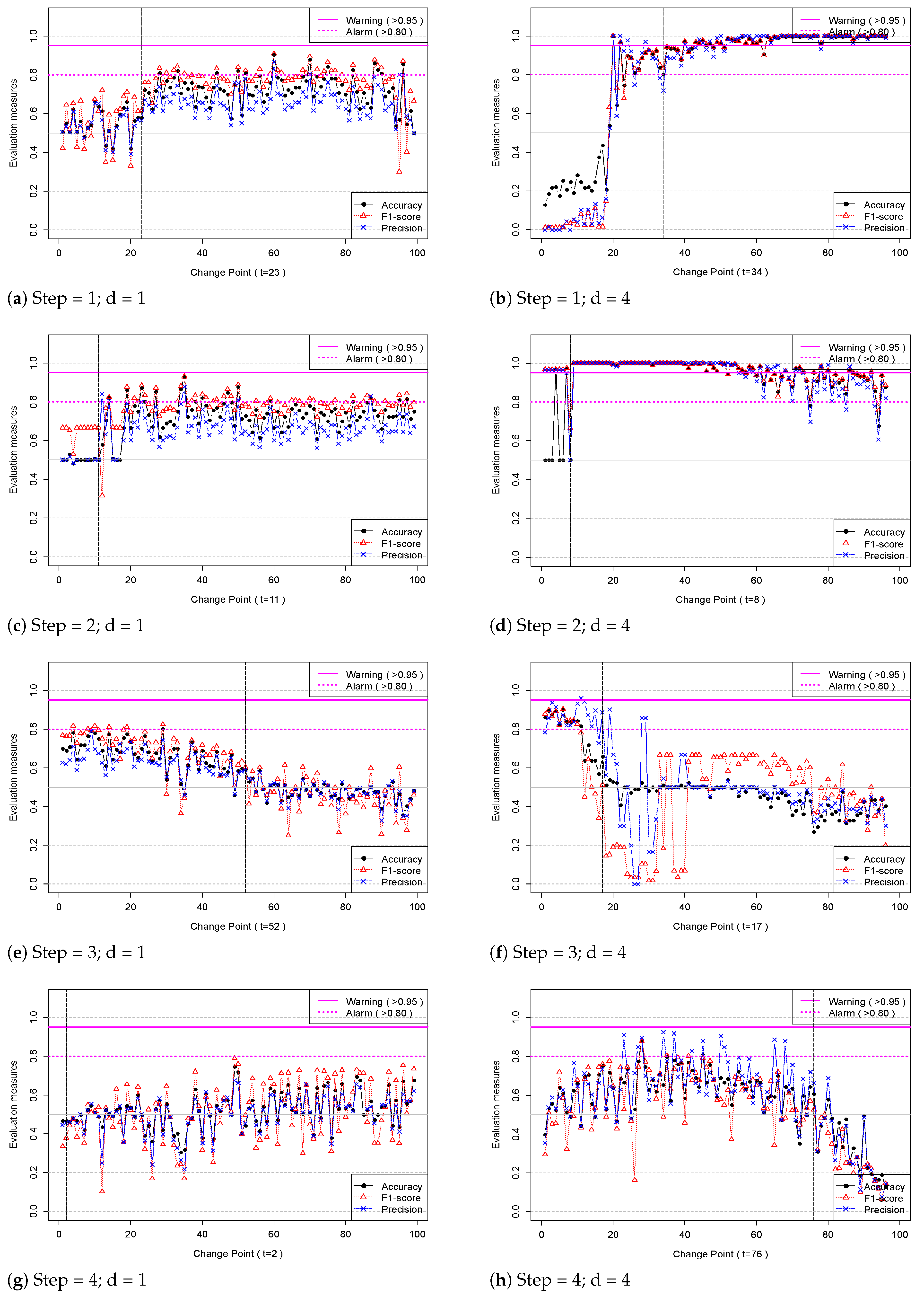
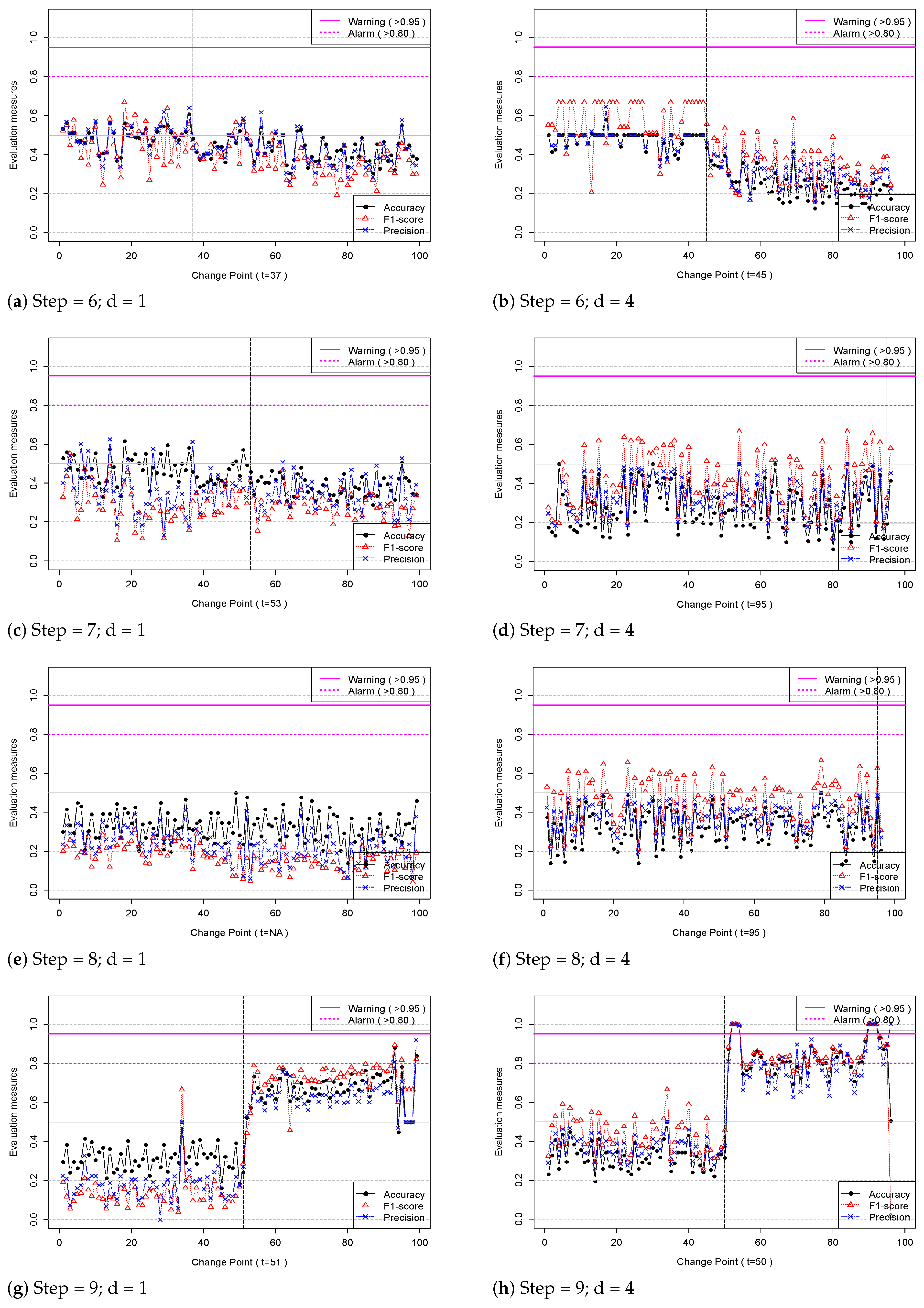
To decide which are the best fitting parameters for the CNN model, the training dataset was split randomly into 70% for the training and 30% for validation. Figure 7 shows the validation loss and accuracy of the training dataset in the case where changes in equipment status cannot be captured. Training loss decreases, but validation loss continues to increase. The accuracy of the training dataset approaches 0.8, but the validation accuracy is below 0.5. This means that the CNN model has low predictive power on new datasets. The algorithm saved the parameters of each epoch and was able to determine which epoch was the best. Figure 8 shows the validation loss and accuracy of the training dataset in the case where changes in equipment status can be captured. It shows that training and validation loss continuously decreases during the training process and converges close to 0. Figure 8 shows that the validation accuracy reached the highest level at epoch 40, then changed slightly. Figure 9 shows the measurement change from Step 1 to Step 4 in Figure 9a–j. As Step 5 has a similar trend to Steps 4 and 6, a graph is not shown. As shown in Figure 9a, the evaluation measure shows a fluctuation around 0.50, so it is not possible to distinguish between the pseudo-labeled PN and PA datasets. Based on change point analysis, t = 23 was determined to be the change point. Around this point, the equipment status changed and continues to change. Furthermore, the fact that the classification accuracy is above 0.80 can be interpreted as a change in equipment status rather than a random change. When , the phenomenon is more obvious than when it is . A change in the overall equipment status is better captured with because a wider range of equipment changes are explored than with . The same phenomenon can also be seen in Figure 9c,d. At and , the evaluation measure decreases, as can be seen in Figure 9e,f. CNN’s classification algorithm cannot detect any differences in equipment status as a result of this. The results are similar in Figure 9g–h and Figure 10a–f. A characteristic of the evaluation measures is the wide fluctuations in and but the stability of accuracy values. It can be seen in Figure 10g,h that interesting changes have occurred in the evaluation measure values. After t is 50, there is a rapid change in equipment status, which was not evident before. In this step, the gearbox tooth is actually missing. It would have been impossible to prevent a catastrophic failure before t was 50 since changes in the evaluation measure were not identified until t was 50. At the point of catastrophic failure, results in an evaluation measure less than 0.80. In the case of , the evaluation measure has a value of 1.0 and shows two distinct peaks. A constant interval (d) between PN and PA makes it possible to detect meaningful changes within that interval rather than cumulative changes. The d value of the abnormality monitoring system will depend on its design purpose. A large d value makes meaningful interpretation difficult because the comparison is with a point in time that is far from the present. Alternatively, if the d value is too small, it is difficult to capture equipment changes sensitively. The optimal d value for equipment monitoring remains a future task.
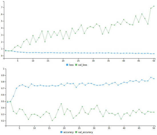
Figure 7.
Training and Validation loss, accuracy during training process at Step 1 (case 1).
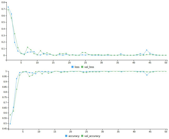
Figure 8.
Training and Validation loss, accuracy during training process at Step 1 (case 2).
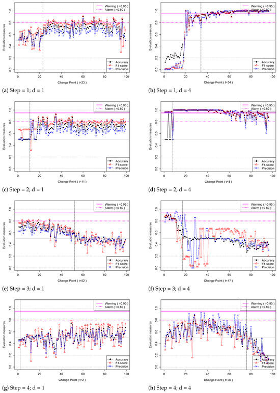
Figure 9.
Evaluation measures for the CNN (Euler method); Step = 1, 2, 3, 4, d = 1, 4.
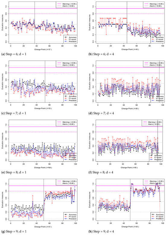
Figure 10.
Evaluation measures for the CNN (Euler method); Step = 6, 7, 8, 9, d = 1, 4.
Table 2 shows the overall results. A large difference between the average value of accuracy before and after the change point means the change in equipment status is large. The difference () in average accuracy before and after the change point for each step can be seen in Table 2. The value was larger when than when , which can be interpreted as more sensitive detection of abnormal signals when . When the alarm level was set to 0.80, an alarm occurred at Steps 1, 2, 3, and 9 for and at Steps 1, 2, 3, 4, and 9 for . When the warning level was set to 0.95, a warning did not appear in any step for , but a warning occurred in Steps 1, 2, and 9 when . In conclusion, we know that when , abnormal signals were detected faster and more sensitively than when . It is necessary to conduct a complementary analysis rather than find the best d value because the characteristics of the information differ depending on the d value. Depending on the d value, a change in a narrow area may be sensitive to changes in a wider area, whereas a change in a broader area may be sensitive to changes in a narrow area. As a result, selecting d as a large value will enable you to see the trend of the overall change. By selecting a small value for d, you will see the trend focusing on the current change rather than the accumulated change. By using , we were able to obtain more useful alarm and warning information in this paper.

Table 2.
Overall results from the experiment.
6. Discussion and Conclusions
Most of the previous studies about equipment monitoring were conducted under the assumption that labels indicating equipment failures could also be collected when collecting data. In cases where data were collected without labels, research was mainly conducted to explore outliers rather than equipment monitoring problems. In the former case, various types of failure were arbitrarily generated in the laboratory; failure labels were assigned to the equipment data collected, and a supervised learning algorithm was applied. However, because various types of failure occur intermittently in the field, labeled data sufficient for supervised learning is rarely collected. Additionally, because the results obtained from research on detecting outliers in equipment data do not indicate equipment failure, fault alarms are often generated. In the case of equipment condition monitoring using the pseudo-label technique proposed in this paper, equipment data collected in unlabeled form were targeted, but normal/abnormal pseudo-labels were assigned to enable the use of various classification algorithms. We proposed a procedure for generating an alarm by monitoring the performance change trends in various classifiers, and we verified its usefulness by applying it to data collected after equipment failure. In this paper, we briefly reviewed recent research to diagnose equipment status based on classification learning. We collected vibration signals from a test rig manufactured to resemble field equipment, assigned pseudo-labels with the Euler method, and observed changes in the classification performance index of the CNN classifier.
In summary, this article contributed to and achieved the following results. First, we proposed assigning pseudo-labels to vibration data collected without labels regarding abnormal equipment conditions. Based on a labeled dataset, we learned a CNN classifier and analyzed the classification accuracy of the model. An alarm is generated if the classification accuracy surpasses 0.80 and a warning signal if it surpasses 0.95. Experimental data were divided into 10 sections called Steps. Using pseudo-labels in Steps 1 to 3, changes in equipment status were detected based on monitoring classification accuracy. In Steps 4 to 8, there was no significant change in status, but in Step 9, a catastrophic failure occurred, and classification accuracy rapidly changed. In this paper, it was confirmed that the d value is one of the parameters of the Euler method that affects the sensitivity of capturing changes in the state of equipment. Results showed that when interval parameter , the change in accuracy was greater than when , and alarm and warning performance was also better. The interval parameter is related to latency in the effect of an equipment failure, and it is important to monitor equipment status efficiently. A classification-based equipment status diagnosis model using pseudo-labels provides meaningful alarm and warning information for each step, but why the alarm occurred is unknown. A promising future study could apply AI to explain the reason the CNN classifier judged the data to be normal or abnormal. If classifier performance is improved by activating a specific frequency region in the CWT image of the vibration signal, fault identification will be possible beyond merely detecting the fault. In the classification-based equipment status diagnosis model, meaningful alarm information was provided for each step, but as future research topics, explanatory research is required for the process of separately extracting and selecting time domain and frequency domain features that can explain changes.
Author Contributions
Conceptualization, M.-K.S. and W.-Y.Y.; methodology, M.-K.S. and W.-Y.Y.; software, M.-K.S.; formal analysis, M.-K.S.; investigation, M.-K.S.; resources, M.-K.S.; data curation, M.-K.S.; writing—original draft, M.-K.S. and W.-Y.Y.; writing—review and editing, W.-Y.Y.; visualization, M.-K.S.; supervision, W.-Y.Y.; project administration, W.-Y.Y. All authors have read and agreed to the published version of the manuscript.
Funding
This research received no external funding.
Institutional Review Board Statement
Not applicable.
Informed Consent Statement
Not applicable.
Data Availability Statement
The data presented in this study are available upon request from the corresponding author. The data are not publicly available due to laboratory regulations.
Conflicts of Interest
Author Myung-Kyo Seo was employed by the company POSCO. The remaining authors declare that the research was conducted in the absence of any commercial or financial relationships that could be construed as a potential conflict of interest.
Abbreviations
The following abbreviations are used in this manuscript:
| AI | Artificial Intelligence |
| ML | Machine Learning |
| Cp | Change point |
| CWT | Continuous Wavelet Transform |
| CNN | Convolutional Neural Network |
| CMS | Condition Monitoring System |
| DCP | Change point Difference |
| DS | Drive Side |
| NDS | Non-Drive Side |
| PN | Pseudo-Normal |
| PA | Pseudo-Abnormal |
| FC | Fully Connected Layer |
| ReLU | Rectified Linear Unit |
| SVM | Support Vector Machine |
| AE | Auto Encoder |
| LSTM | Long Short-Term Memory |
| ODR | Omnidirectional regenerator |
| GMM | Gaussian Mixture Model |
| JTFA | Joint Time-Frequency Analysis |
| FEMP | The Federal Energy Management Program |
| WT | Wavelet Transform |
References
- Yacout, S. Fault detection and Diagnosis for Condition Based Maintenance Using the Logical Analysis of Data. In Proceedings of the 40th International Conference on Computers and Industrial Engineering Computers and Industrial Engineering (CIE), Awaji, Japan, 25–28 July 2010; pp. 1–6. [Google Scholar]
- Farina, M.; Osto, E.; Perizzato, A.; Piroddi, L.; Scattolini, R. Fault detection and isolation of bearings in a drive reducer of a hot steel rolling mill. Control Eng. Pract. 2015, 39, 35–44. [Google Scholar] [CrossRef]
- Jardine, A.K.S.; Lin, D.; Banjevic, D. A review on machinery diagnostics and prognostics implementing condition-based maintenance. Mech. Syst. Signal Process. 2006, 20, 1483–1510. [Google Scholar] [CrossRef]
- Chen, Z.; Li, C.; Sanchez, R.V. Gearbox fault identification and classification with convolutional neural networks. Shock Vib. 2015, 2015, 390134. [Google Scholar] [CrossRef]
- Jing, L.; Zhao, M.; Li, P.; Xu, X. A CNN based feature learning and fault diagnosis method for the condition monitoring of gearbox. Measurement 2017, 111, 1–10. [Google Scholar] [CrossRef]
- Seo, M.K.; Yun, W.Y. Clustering-based monitoring and fault detection in hot strip rolling mill. J. Korean Soc. Qual. Manag. 2017, 45, 298–307. [Google Scholar] [CrossRef]
- Seo, M.K.; Yun, W.Y. Clustering-based hot strip rolling mill diagnosis using Mahalanobis distance. J. Korean Inst. Ind. Eng. 2017, 43, 298–307. [Google Scholar]
- Lee, J.W.; Chon, H.S.; Kwon, D.I. Research trends and analysis in the field of fault diagnosis. Korean Soc. Mech. Eng. (Mech. J.) 2016, 56, 37–40. [Google Scholar]
- Lee, T.H.; Yu, E.S.; Park, K.Y.; Yu, S.S.; Park, J.P.; Mun, D.W. Detection of Abnormal Ship Operation using a Big Data Platform based on Hadoop and Spark. Korean Soc. Manuf. Process Eng. 2019, 18, 82–90. [Google Scholar] [CrossRef]
- Heng, A.; Zhang, S.; Tan, A.C.C.; Matthew, J. Rotating machinery prognostics: State of the art, challenges and opportunities. Mech. Syst. Signal Process. 2009, 23, 724–739. [Google Scholar] [CrossRef]
- Ince, T.; Kiranyaz, S.; Eren, L.; Askar, M.; Gabbouj, M. Real-time motor fault detection by 1-D convolutional neural networks. IEEE Trans. Ind. Electron. 2016, 63, 7067–7075. [Google Scholar] [CrossRef]
- Lupea, L.; Lupea, M. Detecting Helical Gearbox Defects from Raw Vibration Signal Using Convolutional Neural Networks. Sensors 2023, 23, 8769. [Google Scholar] [CrossRef] [PubMed]
- Hu, P.; Zhao, C.; Huang, J.; Song, T. Intelligent and Small Samples Gear Fault Detection Based on Wavelet Analysis and Improved CNN. Processes 2023, 11, 2969. [Google Scholar] [CrossRef]
- Abdeljaber, O.; Avci, O.; Kiranyaz, S.; Gabbouj, M.; Inman, D.J. Real-time vibration-based structural damage detection using one-dimensional convolutional neural networks. J. Sound Vib. 2017, 388, 154–170. [Google Scholar] [CrossRef]
- Park, J.S. Wafer map-based defect Detection Using Convolutional Neural Networks. J. Korean Inst. Ind. Eng. 2018, 44, 249–258. [Google Scholar]
- Perera, L.P.; Brage, M. Data analysis on marine engine operating regions in relation to ship navigation. Ocean Eng. 2018, 128, 163–172. [Google Scholar]
- Jeong, H.; Park, S.; Woo, S.; Lee, S. Rotating machinery diagnostics using deep learning on orbit plot images. Procedia Manuf. 2016, 5, 1107–1118. [Google Scholar] [CrossRef]
- Jung, J.H.; Jeon, B.C.; Youn, B.D.; Kim, M.; Kim, D.; Kim, Y. Omnidirectional regeneration (ODR) of proximity sensor signals for robust diagnosis of journal bearing systems. Mech. Syst. Signal Process. 2017, 90, 189–207. [Google Scholar] [CrossRef]
- Gao, D.; Zhu, Y.; Wang, X.; Yan, K.; Hong, J. A fault diagnosis method of rolling Bearing Based on Complex Morlet CWT and CNN. In Proceedings of the Prognostics and System Health Management Conference (PHM-Chongqing), Chongqing, China, 26–28 October 2018; pp. 1101–1105. [Google Scholar]
- Lee, J.H.; Okwuosa, C.N.; Hur, J.W. Extruder Machine Gear Fault Detection Using Autoencoder LSTM via Sensor Fusion Approach. Inventions 2023, 8, 140. [Google Scholar] [CrossRef]
- Ramteke, D.S.; Parey, A.; Pachori, R.G. A New Automated Classification Framework for Gear Fault Diagnosis Using Fourier–Bessel Domain-Based Empirical Wavelet Transform. Machines 2023, 11, 1055. [Google Scholar] [CrossRef]
- Lee, S.H.; Youn, B.D. Industry 4.0 and direction of failure prediction and health management technology (PHM). J. Korean Soc. Noise Vib. Eng. 2015, 21, 22–28. [Google Scholar]
- Pecht, M.G.; Kang, M.S. Prognostics and Health Management of Electronics-Fundamentals Machine Learning, and the Internet of Things; John Wiley and Sons: Hoboken, NJ, USA, 2008; pp. 23–56. [Google Scholar]
- Yang, B.S.; Widodo, A. Introduction of intelligent Machine Fault Diagnosis and Prognosis; Nova Science Publishers: Hauppauge, NY, USA, 2009; pp. 23–76. [Google Scholar]
- Choi, J.H. A review on prognostics and health management and its application. J. Aerosp. Syst. Eng. 2014, 38, 7–17. [Google Scholar]
- Philip, M.G.; Richard, J.G.; John, I.H. Fundamentals of Fluid Mechanics; Addison-Wesley: Boston, MA, USA, 2009. [Google Scholar]
- Liang, P.L.; Chao, W.; Jun, Y.; Zhixin, Y. Intelligent fault diagnosis of rotating machinery via wavelet transform, generative adversarial nets and convolutional neural network. Measurement 2020, 159, 107768. [Google Scholar] [CrossRef]
- Huang, L.; Wang, J. Forecasting energy fluctuation model by wavelet decomposition and stochastic recurrent wavelet neural network. Neurocomputing 2018, 309, 70–82. [Google Scholar] [CrossRef]
- Lee, J.W.; Lee, H.W.; Yoo, C.S. Selection of mother wavelet for bivariate wavelet analysis. J. Korea Water Resour. Assoc. 2019, 52, 905–916. [Google Scholar]
- Liu, T.; Fang, S.; Zhao, Y.; Wang, P.; Zhang, J. Implementation of training convolutional neural Networks. arXiv 2015, arXiv:1506.01195. [Google Scholar]
- Chollet, F. Deep Learning with R; Manning: Shelter Island, NY, USA, 2018. [Google Scholar]
Disclaimer/Publisher’s Note: The statements, opinions and data contained in all publications are solely those of the individual author(s) and contributor(s) and not of MDPI and/or the editor(s). MDPI and/or the editor(s) disclaim responsibility for any injury to people or property resulting from any ideas, methods, instructions or products referred to in the content. |
© 2024 by the authors. Licensee MDPI, Basel, Switzerland. This article is an open access article distributed under the terms and conditions of the Creative Commons Attribution (CC BY) license (https://creativecommons.org/licenses/by/4.0/).

