Article

Stripe-Assisted Global Transformer and Spatial–Temporal Enhancement for Vehicle Re-Identification

School of Intelligent Systems Engineering, Shenzhen Campus of Sun Yat-sen University, Shenzhen 510275, China
*
Author to whom correspondence should be addressed.
Appl. Sci. 2024, 14(10), 3968; https://doi.org/10.3390/app14103968
Submission received: 22 March 2024 / Revised: 5 May 2024 / Accepted: 6 May 2024 / Published: 7 May 2024
(This article belongs to the Section Transportation and Future Mobility)

Abstract

:
As a core technology in intelligent transportation systems, vehicle re-identification has attracted growing attention. Most existing methods use CNNs to extract global and local features from vehicle images and roughly integrate them for identifying vehicles, addressing intra-class similarity and inter-class difference. However, a significant challenge arises from redundant information between global and local features and possible misalignment among local features, resulting in suboptimal efficiency when combined. To further improve vehicle re-identification, we propose a stripe-assisted global transformer (SaGT) method, which leverages a dual-branch network based on transformers to learn a discriminative whole representation for each vehicle image. Specifically, one branch exploits a standard transformer layer to extract a global feature, while the other branch employs a stripe feature module (SFM) to construct stripe-based features. To further facilitate the effective incorporation of local information into the learning process of the global feature, we introduce a novel stripe-assisted global loss (SaGL), which combines ID losses to optimize the model. Considering redundancy, we only use the global feature for inference, as we enhance the whole representation with stripe-specific details. Finally, we introduce a spatial-temporal probability (STPro) to provide a complementary metric for robust vehicle re-identification. Extensive and comprehensive evaluations on two public datasets validate the effectiveness and superiority of our proposed method.

1. Introduction

With the rapid increase in number of vehicles, the establishment of intelligent transportation systems (ITS) has become increasingly essential. Vehicle re-identification plays a crucial role in ITS by aiming to retrieve all the images of a given query vehicle identity [1,2,3,4,5,6,7], contributing significantly to applications such as suspicious vehicle tracking, vehicle event detection, and vehicle counting [8]. While license plates are commonly used identifiers for vehicles, real-world road surveillance systems often face challenges such as challenging angles and lighting conditions, making accurate license plate recognition difficult. Additionally, intentional obstruction, forgery, and privacy concerns associated with license plates pose significant challenges for vehicle re-identification using them [9]. Consequently, the visual features of vehicles are explored as an alternative to license plates for vehicle re-identification.
With the significant progress of deep learning in computer vision, many methods [10,11,12,13,14,15,16,17,18] now utilize neural networks to adaptively extract high-level features from vehicle images, making them a primary and efficient approach for vehicle re-identification. Some methods [10,11,12,13] focus on embedding a vehicle image into a global feature using CNNs. Nevertheless, they underperform when different vehicles share significantly similar appearance attributes (e.g., Figure 1a) or when the same vehicle exhibits diverse appearances (e.g., Figure 1b), namely, the inter-class similarity and the intra-class difference issues. As shown in Figure 1a, the two different vehicles are difficult to distinguish by their overall appearance but can be by local details. Therefore, most methods [14,15,16,19,20,21,22,23] extract local features from regions and combine them with the global feature to enhance vehicle representation. Still, as depicted in Figure 1b, the regions of local details in different images of the same vehicle do not always correspond, which means that their local features are not inherently aligned. Thus, when local features are conventionally used during the inference stage, irrelevant information caused by misalignment may be introduced. Furthermore, crudely combining the global feature with local features will result in redundancy, as there is some overlap in information between them.
In addition to visual features, other cues are essential to provide complementary information for vehicle re-identification. Unlike the random movement of humans, the movement of vehicles in real-world traffic scenarios is restricted by road topology and traffic rules. This suggests that we can filter vehicle images with the help of spatial–temporal information to achieve more robust vehicle re-identification. Although some methods [10,24,25,26,27] have attempted to use statistical means to model spatial–temporal relations or constraints to refine the retrieval results of vehicles, there is still a need for a comprehensive exploration of both spatial–temporal pattern mining and its integration with visual features.
Considering the above-mentioned issues, we proposed a stripe-assisted global transformer (SaGT) method that guides the global feature to focus on discriminative details from local region representations. Concretely, we design a dual-branch architecture to learn global and local features based on the pure vision transformer (ViT). Following the ViT, we first split the images into patches and embed them with a transformer encoder. Then, we design a stripe feature module (SFM) in one branch to construct stripe-based features and employ a transformer layer to obtain a global representation in the other one. To encourage the model to learn regional features to enrich the whole representation, we further design a stripe-assisted global loss (SaGL). In this way, we can only use the global feature with key parts’ details for vehicle re-identification, avoiding the redundancy and misalignment problems of fusing local features. Furthermore, we introduce spatial–temporal probability (STPro) based on kernel density estimation and fuse it with a visual feature distance as the synthesized similarity of vehicles. Comprehensive evaluations demonstrate that the global feature can learn more details when guided and that STPro can provide complements for vehicle re-identification, effectively.
Our main contributions are summarized as follows:
(1)
We propose a novel SaGT method for vehicle re-identification that learns a discriminative global feature with the assistance of local feature learning, while also considering the redundancy, thereby only using the global feature for inference.
(2)
We design an SFM to construct stripe-based features that effectively capture details in stripe regions. Additionally, we introduce an SaGL to encourage the global feature to learn discriminative information from stripe-based features.
(3)
We introduce STPro to offer an additional metric to enhance vehicle re-identification relying on only visual features. We also explore the fusion of the visual feature metric and STPro to further improve vehicle re-identification.
The rest of this paper is structured as follows. Section 2 provides an overview of related works. Our proposed approach is detailed in Section 3. In Section 4, the experimental results are presented and discussed. Finally, Section 5 concludes this paper.

2. Related Work

2.1. Visual Feature-Based Vehicle Re-Identification

Vehicle re-identification methods using CNNs to extract visual features can be mainly summarized into two categories: global feature-based and local feature-based methods. The former extracts global representations to describe a vehicle. For example, Jiang et al. [10] presented a multi-branch architecture that extracted color, model, and appearance features to comprehensively characterize a vehicle. Similarly, Li et al. [11] introduced the DF-CVTC (Deep Feature with Camera Views, Vehicle Types, and Colors) for vehicle re-identification. To incorporate viewpoint information, Li et al. [12] introduced a method named Viewpoint-Aware Re-Identification (VARID), which employed viewpoint clustering and deep metric learning to acquire discriminative features.
The local feature-based methods concentrate on capturing intricate details from specific regions through either a uniform partition or a predefined key part approach to identify similar vehicles. For example, Chen et al. [19] exploited a Partition and Reunion Network (PRN) that uniformly divided the feature map based on height and width dimensions to obtain local features for vehicle re-identification. Additionally, the DPGM [14] combined the local features split from the same two directions as PRN with a global feature to represent vehicles. In particular, inspired by the PCB [28] designed for person re-identification, the SAN [23] constructed stripe-based features for vehicle re-identification. Like PRN and DPGM, the SAN divided the global feature map from the height dimension into several average part-level features, called stripe-based features. In contrast to these methods mentioned above, Zhang et al. [15] employed an SSD detector to detect 16 vehicle parts and extracted local features from these parts. Liu et al. [16] proposed a Parsing-Guided Cross-Part Reasoning Network (PCRNet), leveraging an image segmentation model to identify predefined local regions and capture details from these regions. However, uniform partitioning leads to a misalignment issue, and predefined key part methods typically rely on an additional detection module, imposing significant annotation and computational burdens. Furthermore, redundancy exists in information between global and local features. Their fusion and use in the inference stage may result in inefficiency, as they incur substantially higher storage costs but yield only marginally improved performance.

2.2. Spatial–Temporal Information-Based Vehicle Re-Identification

While local feature-based methods excel in capturing intricate details, some methods also attempt to explore spatial–temporal information to improve vehicle re-identification. For example, Shen et al. [24] utilized the Markov random field chain to formulate candidate visual–spatial–temporal paths for pairs of vehicles, and then introduced a Siamese–CNN+Path–LSTM model to generate similarity scores for vehicle re-identification, which was the first work to introduce spatial–temporal cues for vehicle re-identification. Lv et al. [25] constructed a maximum transfer time matrix between pairs of cameras, utilizing it to filter gallery images with transfer times exceeding the corresponding matrix values. Jiang et al. [10] observed that the same vehicle shared a smaller space distance and time interval, and they modeled the spatial–temporal relationship to re-rank vehicle re-identification results based on visual features. However, the Siamese–CNN+Path–LSTM model implicitly combined spatial–temporal and visual cues for vehicle re-identification, which lacked interpretability. Furthermore, relying on empirical assumptions or observations, the latter two methods roughly modeled spatial–temporal information of vehicles as constraints to filter unreasonable images, which still faced challenges in complex scenarios. On one hand, they performed limitedly because empirical assumptions or observations were not always accurate in complex cases. On the other hand, they separately utilized the visual and spatial–temporal cues for vehicle re-identification, and the improvement from introducing spatial–temporal information was ineffective. Instead, kernel density estimation (KDE) can flexibly capture deeper characteristics of spatial–temporal data distribution for vehicles by estimating the probability density function in a non-parametric manner. Consequently, leveraging KDE, we construct a fine-grained spatial–temporal probability and fuse it with a visual feature distance to improve vehicle re-identification.

2.3. Vision Transformers

The transformer [29] was originally introduced for machine translation. Dosovitskiy et al. [30] extended its application to images, introducing the vision transformer (ViT) for image classification. Subsequently, various adaptations of transformers for vehicle re-identification have been proposed. For example, Yu et al. [18] proposed a Vehicle Attribute Transformer (VAT), which incorporated color, model, and viewpoint embeddings into a unified feature for effective vehicle re-identification. Shen et al. [31] innovatively designed a Graph Interactive Transformer (GiT), leveraging a combination of a graph network and a transformer to enhance cooperation between local and global features, thereby improving vehicle re-identification. Li et al. [32] introduced a Multi-Scale Knowledge-Aware Transformer (MsKAT) to eliminate state interference (e.g., camera and viewpoint) and gather attribute information (e.g., color and type) for reliable representations of vehicle images. Different from these methods, we employ a ViT to construct stripe-based features that enrich the global feature for vehicle re-identification. We additionally introduce the SaGL to optimize the model. During inference, we exclusively use the global feature, resulting in reduced computational and storage requirements.

3. Methodology

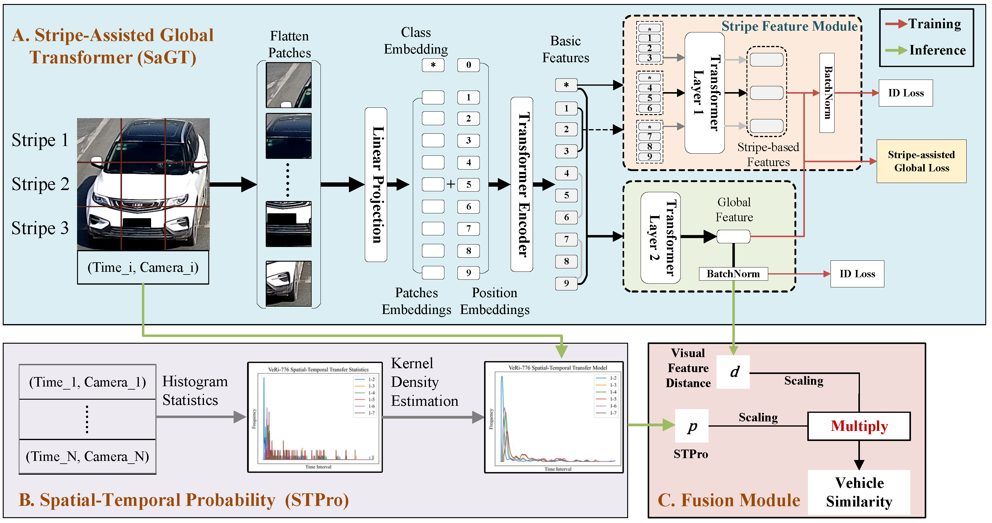
Vehicle re-identification is a retrieval task, and its key to problem-solving is constructing a judgment basis for identifying vehicles. Considering the visual and spatial–temporal cues of vehicles, we extract their visual features and STPro for vehicle re-identification. As illustrated in Figure 2, our approach comprises two streams: visual features and STPro. Within the visual feature stream, we exploit an SaGT that contained a transformer encoder for embedding basic features, an SFM for constructing stripe-based features, and a standard transformer layer for extracting a global feature. All features are first passed through the batch normalization layer (BN) and then used to calculate the ID loss. Meanwhile, the SaGL is directly calculated by the original global and stripe-based features. In the STPro stream, the pattern of spatial–temporal transfer for vehicles is based on the kernel density estimation model. Finally, during inference, the visual (global) feature distance and STPro corresponding to the pair of query and gallery images are fused to obtain the final similarity of the pair.

3.1. SaGT

3.1.1. Embedding Basic Features

Consider a vehicle image X R H × W × C , where H, W, and C denote the height, width, and the number of channels of images, respectively. Following the ViT, we first split the image into N patches x p R P × P × C , where N = H P × W P , ( P , P ) is the size of each patch. Then, we flatten each patch and map it to 1D with a trainable linear function F l ( · ) . Furthermore, we also prepend a learnable class embedding x c l s as the global feature and add a 1D learnable position embedding E p o s to retain spatial information. Therefore, the input Z 0 of the transformer encoder can be expressed as follows:
Z 0 = [ x c l s , F l ( x p 1 ) , F l ( x p 2 ) , , F l ( x p N ) ] + E p o s ,
where x c l s R 1 × D and E p o s R ( N + 1 ) × D .
Finally, the basic features E b of image patches are generated by a transformer encoder including L standard transformer layers, which is described in Equation (3). The transformer layer consists of two layer-normalization (LN) units, a multi-head self-attention (MHSA), and a multi-layer perceptron (MLP) with two hidden layers, detailed in Equation (2) as follows:
Z i = MHSA ( LN ( Z i 1 ) ) + Z i 1 , Z i = MLP ( LN ( Z i ) ) + Z i ,
E b = Z L ,
where Z i R ( N + 1 ) × D is the output of the ith transformer layer.

3.1.2. Extracting Global and Stripe-Based Features

From Figure 2, we employ a transformer layer to encode the basic features E b , and the resulting class embedding serves as the global feature f g of the vehicle image, which is described in Equation (4) as follows:
E g = MHSA ( LN ( E b ) ) + E b , E g = MLP ( LN ( E g ) ) + E g , f g = e g 0 ,
where E g = e g 0 , e g 1 , , e g N .
Meanwhile, we also designed an SFM to construct stripe-based features, capturing local details from specific stripe regions. As depicted in Figure 2, the SFM utilizes a transformer layer to encode patch embeddings from the identical stripe region, along with an additional class embedding x ˜ c l s to represent the stripe-based feature. The class embedding is initialized by the basic class embedding e b 0 , as expressed in Equation (7). As described in Section 3.1.1, the vehicle image is divided uniformly into N patches. Assume that K stripe-based features are constructed along the vertical direction, resulting in M = N K patches in each horizontal stripe region. Note that proper K must ensure that M is an integer. The embeddings of the jth horizontal stripe X s j can be formed according to Equation (5) as follows:
X s j = e b ( j 1 ) M + 1 , e b ( j 1 ) M + 2 , , e b j M ,
where j { 1 , , K } . Then, the input Z ˜ 0 j for the jth stripe fed to the SFM can be described in Equation (6):
Z ˜ 0 i = x ˜ c l s , x s j , 1 , , x s j , M ,
x ˜ c l s = e b 0 ,
where x ˜ c l s R 1 × D and X s j = [ x s j , 1 , , x s j , M ] . Then, the jth stripe-based feature f l j is produced by the SFM according to Equation (8).
E l , j = MHSA ( LN ( Z ˜ 0 i ) ) + Z ˜ 0 i , E l , j = MLP ( LN ( E l , j ) ) + E l , j , f l j = e l , j 0 ,
where E l , j = e l , j 0 , e l , j 1 , , e l , j M .
Finally, we can obtain K horizontal stripe-based features F l for one vehicle image, i.e., F l = f l 1 , f l 2 , , f l K .

3.1.3. Model Optimization

To optimize the model, we combined the ID loss and SaGL for global and stripe-based feature learning. The global ID loss L I D g based on cross-entropy loss with label smoothing [33] is defined as follows:
L I D g = 1 N i = 1 N m = 1 M log y ^ i [ m ] q ( y i , m ) , y ^ i = softmax FC BN f g i , q ( y i , m ) = ( 1 ε ) 1 | y i = m + ε M ,
where N and M denote the number of training samples and the number of training identity labels, respectively. y ^ i represents the predictive probability distribution over identities of the ith sample, obtained using the softmax function. FC refers to the fully connected layer. f g i is the global feature of the ith sample; y i represents the ground-truth label of the ith sample; q ( y i , m ) is the modified probability of y i ; ( 1 | y i = m ) equals 1 for y i = m and 0 for otherwise; and ε , set to 0.1 in this work, is the weight coefficient of label smoothing.
Similar to the global ID loss, the local ID loss L I D l is described as follows:
L I D l = 1 N × K i = 1 N k = 1 K m = 1 M log y ^ i , k [ m ] q ( y i , m ) , y ^ i , k = softmax FC BN f l k , i ,
where K denotes the number of stripe-based features for each vehicle image. y ^ i , k is the predictive probability distribution over identities corresponding to the kth stripe-based feature of the ith sample, and f l k , i is the kth stripe-based feature of the ith sample; q ( y i , m ) still represents the modified probability of y i and is defined in the same manner as L I D g .
In particular, to encourage the global feature to learn more discriminative details from stripe-based features, we designed an SaGL inspired by the triplet loss. Given a training batch containing M × N vehicle images, with M vehicles identities and N images for each identity, the SaGL L S a G L is defined as follows:
L S a G L = i = 1 M a = 1 N [ m + d ( f g a , i , f g p , i ) + 1 K k = 1 K d ( f l a , i , k , f l p , i , k ) d ( f g a , i , f g n , j ) 1 K k = 1 K d ( f l a , i , k , f l n , j , k ) ] + , p = arg max p ( 1 , , N ) d ( f g a , i , f g p , i ) , n , j = arg min j ( 1 , , M ) n ( 1 , , N ) d ( f g a , i , f g n , j ) ,
where K denotes the number of stripe-based features for each vehicle image. f g x , y denotes the global feature corresponding to the xth image of the yth vehicle in the above-mentioned batch. Similarly, f l x , y , k denotes the kth stripe-based feature corresponding to the xth image of the yth vehicle in the same batch. The function d ( · ) represents the Euclidean distance. The margin m is a hyperparameter set to 0.6 in this work. The notation [ x ] + denotes the maximum value between 0 and x. Note that all features are normalized.
Therefore, the total loss L t o t a l is formulated as follows:
L t o t a l = L I D g + L I D l + L S a G L .

3.2. STPro

To improve vehicle re-identification, we modeled and incorporate spatial–temporal patterns based on KDE. Specifically, we estimated the distribution of vehicle movement times between camera pairs based on the training data. The process is detailed in the following two steps:

3.2.1. Histogram Statistic

We first define image pairs with the same ID as positive pairs. Then, we build the training set T ( c i , c j ) for the camera pair ( c i , c j ) from those positive pairs, which is described as follows:
T ( c i , c j ) = ( t i , t j ) | I D i = I D j ,
where c i , t i , and I D i denote the camera number, timestamp, and identity of the ith training image, respectively. We further count the time interval histogram p ^ ( k | c i , c j ) for camera pair ( c i , c j ) :
p ^ ( k | c i , c j ) = n k m n m ,
where k = | t i t j | Δ t , ( t i , t j ) T ( c i , c j ) , and n k represents the amount in the kth bin. Δ t is the width of the bin.

3.2.2. Kernel Density Estimation

After obtaining the histogram for the camera pair ( c i , c j ) , we smooth it using a Gaussian kernel N ( x | 0 , σ 2 ) with a zero mean and variance σ 2 and estimate its probability. The final STPro model for ( c i , c j ) can be formulated according to Equation (15).
p ( k | c i , c j ) = 1 ω l p ^ ( l | c i , c j ) N ( l k | 0 , σ 2 ) , ω = m p ( m | c i , c j ) .

3.3. Fusion Module

Given two images A and B with timestamp and camera ID, as described in Section 3.1 for the visual feature stream and Section 3.2 for the STPro stream, we can obtain their global features f g A , f g B , and spatial–temporal probability (STPro) p. We then calculate the Euclidean distance d = | | f g A f g B | | 2 between f g A and f g B , which is used for inference when only considering visual features.
Visual feature distance d and STPro p show opposite trends in measuring vehicle similarity. A smaller d means vehicle images are more similar, while a smaller p indicates they are less similar. Furthermore, d and p have different ranges: d ( 0 , ) and p ( 0 , 1 ) . Therefore, we adopted two nonlinear transforms based on the exponential function to scale d and p from 0 to 1 before fusing them, respectively. Concretely, the visual feature distance d and STPro p are scaled according to Equation (16) and Equation (17), respectively.
d = 2 2 e d + 1 ,
where d ( 0 , 1 ) represents the scaled visual feature distance, and e is the Euler number.
p = e p 1 ,
where p ( 0 , 1 ) represents the scaled STPro.
Finally, according to Equation (18), the result of d multiplied by p represents the final similarity S between A and B for vehicle re-identification. The multiplication operation is inspired by the union of independent probabilities, under the assumption that visual features of vehicle images and their spatial–temporal cues are quite independent.
S = d × p .

4. Experiment

We evaluated our proposed method on two large-scale datasets, i.e., VeRi-776 [34] and VehicleID [35]. Similar to previous works [34,35], we employed the mean average precision (mAP) and Rank-1 accuracy as our evaluation metrics.

4.1. Dataset

4.1.1. VeRi-776

The VeRi-776 [34] dataset collected around 50,000 images of 776 vehicles captured by 20 surveillance cameras in real-world traffic scenes. These images were labeled with vehicle ID, color, and model information. Among them, 576 vehicles with a total of 37,746 images were selected for training, and the remaining 11,579 images of 200 vehicles were for testing. Concretely in the testing set, 1678 images of 200 vehicles were selected as query images. Note that during evaluation, for each query image, gallery images captured by the same camera were discarded. Additionally, it provided timestamp and camera location information, crucial for evaluating our STPro method.

4.1.2. VehicleID

The VehicleID [35] dataset captured 221,763 images of 26,267 vehicles from multiple non-overlapping surveillance cameras in real-world scenarios. Each image was also annotated with vehicle ID, color, and model information. Unlike VeRi with multiple different viewpoints, images in VehicleID were taken exclusively from the front or back, with fewer but more drastic changes in viewing angle. Similarly, the dataset was divided into training and testing sets. The training set contained 110,178 images of 13,134 vehicles, while the testing set retained 111,585 images associated with 13,133 vehicles. Three subsets were further extracted from the testing set, i.e., a small subset with 7332 images of 800 vehicles, a medium subset with 12,995 images of 1600 vehicles, and a large subset with 20,038 images of 2400 vehicles. More specifically, for each subset, the gallery set was formed by randomly extracting one image for each vehicle, and the remaining images were used for query set construction. It is important to note that we iteratively constructed each subset and evaluate it 10 times, taking the average result as the final performance. Unfortunately, it provided no timestamp and camera location information to evaluate our STPro method.

4.2. Implementation Details

All our experiments were conducted on eight Nvidia Tesla T4 GPUs with the PyTorch Toolbox. Both training images and testing images were resized to 256 × 256 . The training images were augmented with horizontal flipping and random erasing. Four images for each identity were sampled in a training mini-batch. We employed the stochastic gradient descent (SGD) to optimize our model with 300 epochs, where the momentum and the weight decay were set at 0.9 and 0.0001 , respectively. The learning rate was initialized to 0.045 with a linear warmup and cosine learning rate decay.
For our model, we initialized the 13 transformer layers with the pre-trained weight of the ViT on ImageNet, where 11 transformer layers were utilized to embed the basic features, 1 layer was applied to extract a global feature, and 1 shared layer was employed to construct the stripe-based features. Each transformer layer consisted of an eight-head self-attention module. We split the original image into 256 non-overlapping patches with size 16 × 16 as the input of the model and constructed K = 8 horizontal stripe-based features. The feature dimension was 768. The width of bin Δ t was set to 4 s, and variance σ 2 was set to 100 in the STPro stream.

4.3. Comparisons with State-of-the-Art Methods

We compared our method with some state-of-the-art (SOTA) approaches from the last three years, categorized into three groups: (1) Global feature-based (GF) methods, such as SN [13], VARID [12], VAT [18], and MsKAT [32], mainly concentrate on extracting whole representation for vehicle images. (2) Local feature-based (LF) methods, including DPGM [14], LG-CoT [36], HPGN [37], DFR [38], DSN [39], SFMNet [40], GiT [31], SOFCT [22], MART [41] integrate local features with the global feature to learn reliable vehicle representations. (3) Spatial–temporal (ST) methods, such as DPGM-ST [14] and DFR-ST [38], exploit extra timestamp and camera location information to enhance vehicle re-identification using visual features. The Baseline refers to our model using only a branch for global feature learning without the SFM. Since our method only takes the global feature for inference, we classified it as a GF-based method.

4.3.1. Comparisons on VeRi-776

Table 1 compares the performance of the SOTA methods on VeRi-776. First, our SaGT-ST method demonstrated superior performance by incorporating spatial–temporal information, achieving the highest mAP of 86.59 % and Rank-1 accuracy of 98.75 % . Furthermore, among methods relying solely on visual features, our SaGT method outperformed most GF- and LF-based approaches, securing the fourth place. Specifically, SaGT combined local features to complement global feature learning compared to GF-based methods, while avoiding local feature misalignment issues associated with LF-based methods. However, it is important to note that without considering background interference, SaGT exhibited a relatively lower performance than MART on VeRi-776. Moreover, SaGT exhibited comparatively lower performance than DFR and MsKAT. This difference can be attributed to the integration of attention mechanisms that effectively combine multiple features in DFR and MsKAT. Obviously, the incorporation of spatial–temporal cues significantly enhanced the performance of vehicle re-identification. For example, both DFR-ST and DPGM-ST achieved superior performance compared to their counterparts DFR and DPGM which only adopt visual features. It is noteworthy that, since only the VeRi-776 dataset contained timestamp and camera position information, similar to DGPM-ST and DFR-ST, we also only evaluated our SaGT-ST method on VeRi-776.

4.3.2. Comparisons on VehicleID

Table 2 compares the performance of the SOTA methods on VehicleID. Our SaGT method continued to achieve competitive performance on three subsets of VehicleID. In particular, our SaGT method achieved the highest mAP and Rank-1 on the small subset, the highest mAP and second highest Rank-1 on the medium subset, and the third highest mAP and Rank-1 on the large subset. Compared with other methods that performed well on VeRi, our method was superior on VehicleID. This can be attributed to the fact that VehicleID provides more training data, promoting our model to learn more patterns. Additionally, when vehicle images encounter drastic viewpoint changes in VehicleID, we employed local features to assist SaGT in learning a reliable whole representation, which brought better overall performance than MsKAT and DFR.

4.4. Ablation Study and Analysis

To further analyze the effectiveness of our proposed method, we conducted extensive ablation experiments on VeRi-776 and VehicleID.

4.4.1. Effectiveness of STPro

ST refers to the method employing STPro, while Baseline still indicates that our model solely activates a branch for global feature learning without the SFM. Add and Multiply represent different ways of fusing scaled visual feature distance and scaled STPro. According to Table 3, methods integrated with STPro significantly outperformed those only using visual features, which demonstrates the effectiveness of mining spatial–temporal patterns. When visual appearance features alone prove insufficient for determining a vehicle’s identity, its spatial–temporal cues provide complementary information, thus enhancing vehicle re-identification. Additionally, it is evident that the fusion of visual feature similarity and STPro performed better in a multiplicative manner compared to an additive way. This supports our intuition that the visual features of vehicle images and their spatial–temporal cues are highly independent, hence treating their fusion as a joint probabilistic processing of independent events is justified.

4.4.2. Effectiveness of SFM and SaGL

Table 4 displays the results of the ablation study involving SFM and SaGL on VeRi-776 and VehicleID datasets. SaGT-SFM integrated an SFM into the Baseline, which trained global and local features using the triplet loss, respectively. Compared to SaGT-SFM, the final method SaGT was optimized by an SaGL instead of the triplet loss. As illustrated in Table 4, SaGT-SFM and SaGT significantly outperformed the Baseline method on VeRi-776 and VehicleID, indicating the substantial contribution of effective local feature learning to overall representation enhancement. Furthermore, SaGT exhibited superior performance compared to SaGT-SFM. The advantage can be credited to SaGL, which enables more focused attention on acquiring a discriminative global representation when the model simultaneously learns global and local features, compared to the original triplet loss.
Table 5 shows the performance of different features for inference on VeRi-776. Time represents the average time required to extract features for one image, measured on a Tesla T4 GPU. Storage denotes the storage cost of image features on a 64-bit system. GF and LF refers to combining the global feature distance and the local feature distance for inference by taking their sum. From Table 5, compared to using either GF or LF for inference, fusing them only brought a slight improvement in mAP. This indicated a significant overlap of information between global and local features, namely, redundancy. Moreover, although the fusion or utilization of only LF for inference outperformed GF, their feature dimension also increased by almost eight times, which implied that applications associated with vehicle re-identification would demand eight times more storage space and more computing consumption. This consideration motivated us to choose only a global feature for inference, and SaGT, employing only a global feature, achieved performance similar to the fusion method in SaGT-SFM.

4.4.3. Visualization Analysis

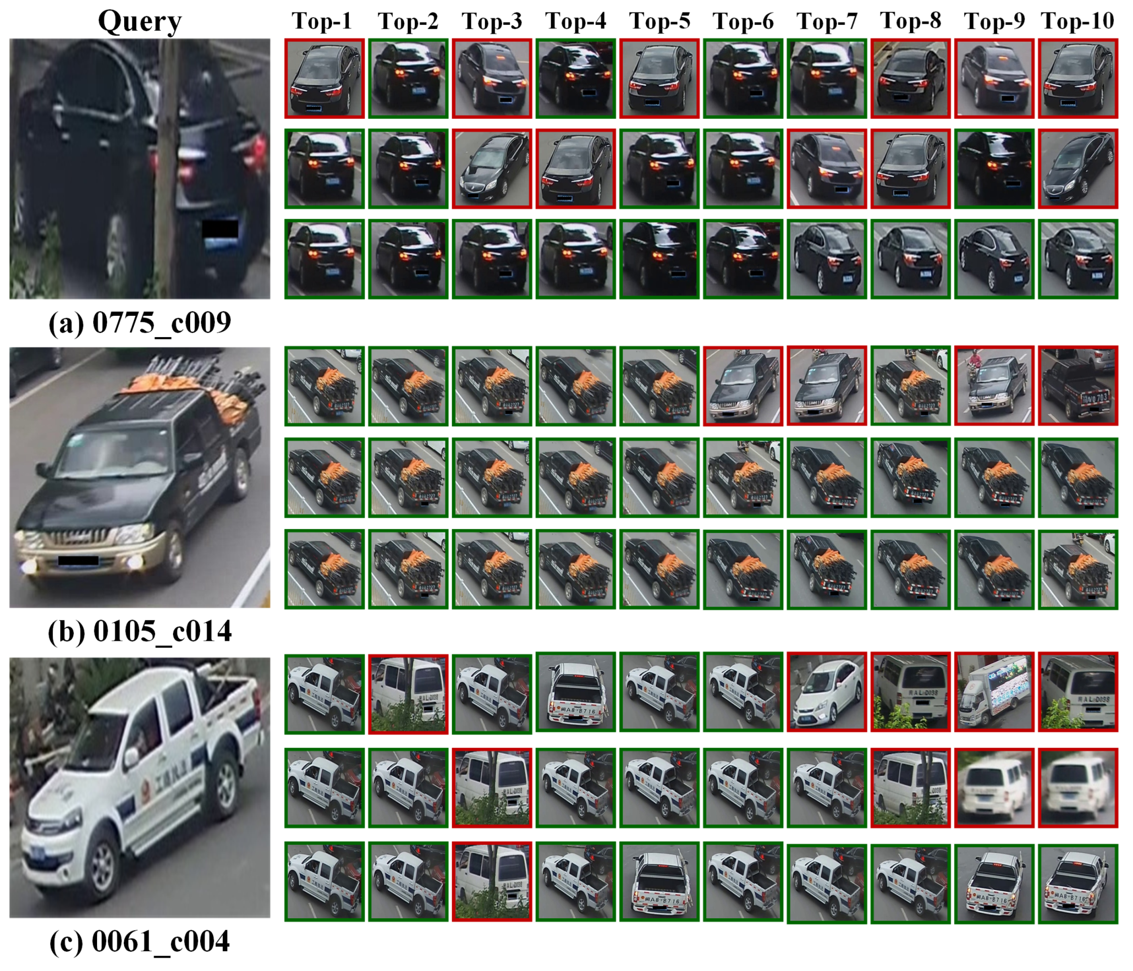
In addition to the ablation study of our proposed method, we visualized the results of vehicle re-identification and Grad-CAM of attention maps to further analyze its effectiveness. Figure 3 presents the top-10 retrieval results of three query images from VeRi-776, where green and red borders denote correct and incorrect retrieval results, respectively. It is clear that both Baseline and SaGT achieved promising performance in scenarios with slight viewpoint variations (e.g., Figure 3b,c). When vehicle images shared similar appearances, SaGT, capturing crucial local details for accurate identification, yielded a larger number of correct retrieval results than Baseline (e.g., Figure 3b). Nevertheless, in cases involving occlusions and extremely similar appearances (e.g., Figure 3a,c), both Baseline and SaGT, relying solely on visual features, generated great error matches. The introduction of spatial–temporal cues in SaGT-ST significantly improved performance for these challenging scenarios.
Figure 4 shows the Grad-CAM [42] visualization of attention maps. Compared to the Baseline, SaGT paid more attention to local regions with key details, which can provide more discriminative information for the global representation of vehicles. However, both baseline and SaGT were interfered with by irrelevant information, especially the road sign, in the background.

5. Conclusions

In this paper, we proposed an SaGT method to extract a global feature for robust vehicle re-identification. In particular, we designed an SFM to construct stripe-based features and to capture local details. We also implemented an SaGL to ensure that the SFM provided the identity-relevant information in the stripe regions for the global feature, making it more discriminative. Therefore, in the inference stage, we only used the global feature for effective identity matching, while reducing the computing and storage consumption of the method and improving its efficiency in practical applications. Additionally, we enhanced the performance of vehicle re-identification by mining spatial–temporal patterns through kernel density estimation. While extensive experimental evaluations confirmed the effectiveness of our method and demonstrated its superior performance compared to SOTA methods, it is still necessary to further address the significant interference from the background of vehicle images.

Author Contributions

Conceptualization, methodology, software, data curation, writing—original draft, Y.A.; investigation, formal analysis, data curation, X.Z.; funding acquisition, supervision, writing—review and editing, X.T.; data curation, B.S. All authors have read and agreed to the published version of the manuscript.

Funding

The research is supported by the Key-Research and Development Prgoram of Guangdong Province under Grant 2020B0909030005.

Institutional Review Board Statement

Not applicable.

Informed Consent Statement

Not applicable.

Data Availability Statement

We, the authors, will provide the data when the necessary information and data are required.

Conflicts of Interest

The authors declare no conflicts of interest.

References

  1. Khan, S.D.; Ullah, H. A survey of advances in vision-based vehicle re-identification. Comput. Vis. Image Underst. 2019, 182, 50–63. [Google Scholar] [CrossRef]
  2. Lou, Y.; Bai, Y.; Liu, J.; Wang, S.; Duan, L. Veri-wild: A large dataset and a new method for vehicle re-identification in the wild. In Proceedings of the IEEE/CVF Conference on Computer Vision and Pattern Recognition, Long Beach, CA, USA, 15–20 June 2019; pp. 3235–3243. [Google Scholar] [CrossRef]
  3. Bai, Y.; Liu, J.; Lou, Y.; Wang, C.; Duan, L.Y. Disentangled feature learning network and a comprehensive benchmark for vehicle re-identification. IEEE Trans. Pattern Anal. Mach. Intell. 2021, 44, 6854–6871. [Google Scholar] [CrossRef]
  4. He, S.; Luo, H.; Wang, P.; Wang, F.; Li, H.; Jiang, W. Transreid: Transformer-based object re-identification. In Proceedings of the IEEE/CVF International Conference on Computer Vision, Montreal, BC, Canada, 11–17 October 2021; pp. 15013–15022. [Google Scholar] [CrossRef]
  5. Lian, J.; Wang, D.H.; Wu, Y.; Zhu, S. Multi-Branch Enhanced Discriminative Network for Vehicle Re-Identification. IEEE Trans. Intell. Transp. Syst. 2023, 25, 1263–1274. [Google Scholar] [CrossRef]
  6. Sun, K.; Pang, X.; Zheng, M.; Nie, X.; Li, X.; Zhou, H.; Yin, Y. Heterogeneous context interaction network for vehicle re-identification. Neural Netw. 2024, 169, 293–306. [Google Scholar] [CrossRef]
  7. Xu, Z.; Wei, L.; Lang, C.; Feng, S.; Wang, T.; Bors, A.G.; Liu, H. SSR-Net: A Spatial Structural Relation Network for Vehicle Re-identification. ACM Trans. Multimed. Comput. Commun. Appl. 2023, 19, 216. [Google Scholar] [CrossRef]
  8. Wang, H.; Hou, J.; Chen, N. A survey of vehicle re-identification based on deep learning. IEEE Access 2019, 7, 172443–172469. [Google Scholar] [CrossRef]
  9. Guo, H.; Zhu, K.; Tang, M.; Wang, J. Two-level attention network with multi-grain ranking loss for vehicle re-identification. IEEE Trans. Image Process. 2019, 28, 4328–4338. [Google Scholar] [CrossRef]
  10. Jiang, N.; Xu, Y.; Zhou, Z.; Wu, W. Multi-attribute driven vehicle re-identification with spatial-temporal re-ranking. In Proceedings of the 2018 25th IEEE International Conference on Image Processing (ICIP), Athens, Greece, 7–10 October 2018; pp. 858–862. [Google Scholar] [CrossRef]
  11. Li, H.; Lin, X.; Zheng, A.; Li, C.; Luo, B.; He, R.; Hussain, A. Attributes guided feature learning for vehicle re-identification. IEEE Trans. Emerg. Top. Comput. Intell. 2021, 6, 1211–1221. [Google Scholar] [CrossRef]
  12. Li, Y.; Liu, K.; Jin, Y.; Wang, T.; Lin, W. VARID: Viewpoint-aware re-identification of vehicle based on triplet loss. IEEE Trans. Intell. Transp. Syst. 2020, 23, 1381–1390. [Google Scholar] [CrossRef]
  13. Li, K.; Ding, Z.; Li, K.; Zhang, Y.; Fu, Y. Vehicle and person re-identification with support neighbor loss. IEEE Trans. Neural Netw. Learn. Syst. 2020, 33, 826–838. [Google Scholar] [CrossRef]
  14. Chen, X.; Sui, H.; Fang, J.; Feng, W.; Zhou, M. Vehicle re-identification using distance-based global and partial multi-regional feature learning. IEEE Trans. Intell. Transp. Syst. 2020, 22, 1276–1286. [Google Scholar] [CrossRef]
  15. Zhang, X.; Zhang, R.; Cao, J.; Gong, D.; You, M.; Shen, C. Part-Guided Attention Learning for Vehicle Instance Retrieval. IEEE Trans. Intell. Transp. Syst. 2022, 23, 3048–3060. [Google Scholar] [CrossRef]
  16. Liu, X.; Liu, W.; Zheng, J.; Yan, C.; Mei, T. Beyond the parts: Learning multi-view cross-part correlation for vehicle re-identification. In Proceedings of the 28th ACM International Conference on Multimedia, Seattle, WA, USA, 12–16 October 2020; pp. 907–915. [Google Scholar] [CrossRef]
  17. Teng, S.; Zhang, S.; Huang, Q.; Sebe, N. Multi-view spatial attention embedding for vehicle re-identification. IEEE Trans. Circuits Syst. Video Technol. 2020, 31, 816–827. [Google Scholar] [CrossRef]
  18. Yu, Z.; Pei, J.; Zhu, M.; Zhang, J.; Li, J. Multi-attribute adaptive aggregation transformer for vehicle re-identification. Inf. Process. Manag. 2022, 59, 102868. [Google Scholar] [CrossRef]
  19. Chen, H.; Lagadec, B.; Bremond, F. Partition and reunion: A two-branch neural network for vehicle re-identification. In Proceedings of the CVPR Workshops, Long Beach, CA, USA, 16–20 June 2019; pp. 184–192. [Google Scholar]
  20. Wang, H.; Peng, J.; Jiang, G.; Xu, F.; Fu, X. Discriminative feature and dictionary learning with part-aware model for vehicle re-identification. Neurocomputing 2021, 438, 55–62. [Google Scholar] [CrossRef]
  21. Qian, J.; Zhao, J. PFNet: Part-guided feature-combination network for vehicle re-identification. Multimed. Tools Appl. 2024, 1–18. [Google Scholar] [CrossRef]
  22. Yu, Z.; Huang, Z.; Pei, J.; Tahsin, L.; Sun, D. Semantic-Oriented Feature Coupling Transformer for Vehicle Re-Identification in Intelligent Transportation System. IEEE Trans. Intell. Transp. Syst. 2023, 25, 2803–2813. [Google Scholar] [CrossRef]
  23. Qian, J.; Jiang, W.; Luo, H.; Yu, H. Stripe-based and attribute-aware network: A two-branch deep model for vehicle re-identification. Meas. Sci. Technol. 2020, 31, 095401. [Google Scholar] [CrossRef]
  24. Shen, Y.; Xiao, T.; Li, H.; Yi, S.; Wang, X. Learning deep neural networks for vehicle re-id with visual-spatio-temporal path proposals. In Proceedings of the IEEE International Conference on Computer Vision, Venice, Italy, 22–29 October 2017; pp. 1900–1909. [Google Scholar] [CrossRef]
  25. Lv, K.; Du, H.; Hou, Y.; Deng, W.; Sheng, H.; Jiao, J.; Zheng, L. Vehicle Re-Identification with Location and Time Stamps. In Proceedings of the CVPR Workshops, Long Beach, CA, USA, 16–20 June 2019; pp. 399–406. [Google Scholar]
  26. Tong, P.; Li, M.; Li, M.; Huang, J.; Hua, X. Large-scale vehicle trajectory reconstruction with camera sensing network. In Proceedings of the 27th Annual International Conference on Mobile Computing and Networking, New Orleans, LA, USA, 25–29 October 2021; pp. 188–200. [Google Scholar] [CrossRef]
  27. Yao, H.; Duan, Z.; Xie, Z.; Chen, J.; Wu, X.; Xu, D.; Gao, Y. City-scale multi-camera vehicle tracking based on space-time-appearance features. In Proceedings of the IEEE/CVF Conference on Computer Vision and Pattern Recognition, New Orleans, LA, USA, 18–24 June 2022; pp. 3310–3318. [Google Scholar] [CrossRef]
  28. Sun, Y.; Zheng, L.; Yang, Y.; Tian, Q.; Wang, S. Beyond Part Models: Person Retrieval with Refined Part Pooling (and A Strong Convolutional Baseline). In Lecture Notes in Computer Science; Springer International Publishing: Berlin/Heidelberg, Germany, 2018; pp. 501–518. [Google Scholar] [CrossRef]
  29. Vaswani, A.; Shazeer, N.; Parmar, N.; Uszkoreit, J.; Jones, L.; Gomez, A.N.; Kaiser, Ł.; Polosukhin, I. Attention is all you need. In Proceedings of the Advances in Neural Information Processing Systems, Long Beach, CA, USA, 4–9 December 2017; Volume 30. [Google Scholar]
  30. Dosovitskiy, A.; Beyer, L.; Kolesnikov, A.; Weissenborn, D.; Zhai, X.; Unterthiner, T.; Dehghani, M.; Minderer, M.; Heigold, G.; Gelly, S.; et al. An Image is Worth 16 × 16 Words: Transformers for Image Recognition at Scale. In Proceedings of the International Conference on Learning Representations, Addis Ababa, Ethiopia, 26–30 April 2020. [Google Scholar]
  31. Shen, F.; Xie, Y.; Zhu, J.; Zhu, X.; Zeng, H. Git: Graph interactive transformer for vehicle re-identification. IEEE Trans. Image Process. 2023, 32, 1039–1051. [Google Scholar] [CrossRef] [PubMed]
  32. Li, H.; Li, C.; Zheng, A.; Tang, J.; Luo, B. MsKAT: Multi-scale knowledge-aware transformer for vehicle re-identification. IEEE Trans. Intell. Transp. Syst. 2022, 23, 19557–19568. [Google Scholar] [CrossRef]
  33. Szegedy, C.; Vanhoucke, V.; Ioffe, S.; Shlens, J.; Wojna, Z. Rethinking the inception architecture for computer vision. In Proceedings of the IEEE Conference on Computer Vision and Pattern Recognition, Las Vegas, NV, USA, 27–30 June 2016; pp. 2818–2826. [Google Scholar] [CrossRef]
  34. Liu, X.; Liu, W.; Mei, T.; Ma, H. A deep learning-based approach to progressive vehicle re-identification for urban surveillance. In Proceedings of the ECCV 2016, Amsterdam, The Netherlands, 11–14 October 2016; Springer: Berlin/Heidelberg, Germany, 2016; pp. 869–884. [Google Scholar] [CrossRef]
  35. Liu, H.; Tian, Y.; Yang, Y.; Pang, L.; Huang, T. Deep relative distance learning: Tell the difference between similar vehicles. In Proceedings of the IEEE Conference on Computer Vision and Pattern Recognition, Las Vegas, NV, USA, 27–30 June 2016; pp. 2167–2175. [Google Scholar] [CrossRef]
  36. Shi, Y.; Zhang, X.; Tan, X. Local-guided Global Collaborative Learning Transformer for Vehicle Reidentification. In Proceedings of the 2022 IEEE 34th International Conference on Tools with Artificial Intelligence (ICTAI), Macao, China, 31 October–2 November 2022; pp. 793–798. [Google Scholar] [CrossRef]
  37. Shen, F.; Zhu, J.; Zhu, X.; Xie, Y.; Huang, J. Exploring spatial significance via hybrid pyramidal graph network for vehicle re-identification. IEEE Trans. Intell. Transp. Syst. 2021, 23, 8793–8804. [Google Scholar] [CrossRef]
  38. Tu, J.; Chen, C.; Huang, X.; He, J.; Guan, X. DFR-ST: Discriminative feature representation with spatio-temporal cues for vehicle re-identification. Pattern Recognit. 2022, 131, 108887. [Google Scholar] [CrossRef]
  39. Zhu, W.; Wang, Z.; Wang, X.; Hu, R.; Liu, H.; Liu, C.; Wang, C.; Li, D. A Dual Self-Attention mechanism for vehicle re-Identification. Pattern Recognit. 2023, 137, 109258. [Google Scholar] [CrossRef]
  40. Li, Z.; Deng, Y.; Tang, Z.; Huang, J. Sfmnet: Self-guided feature mining network for vehicle re-identification. In Proceedings of the 2023 International Joint Conference on Neural Networks (IJCNN), Gold Coast, Australia, 18–23 June 2023; pp. 1–8. [Google Scholar] [CrossRef]
  41. Lu, Z.; Lin, R.; Hu, H. MART: Mask-aware reasoning transformer for vehicle re-identification. IEEE Trans. Intell. Transp. Syst. 2022, 24, 1994–2009. [Google Scholar] [CrossRef]
  42. Selvaraju, R.R.; Cogswell, M.; Das, A.; Vedantam, R.; Parikh, D.; Batra, D. Grad-cam: Visual explanations from deep networks via gradient-based localization. In Proceedings of the IEEE International Conference on Computer Vision, Venice, Italy, 22–29 October 2017; pp. 618–626. [Google Scholar] [CrossRef]
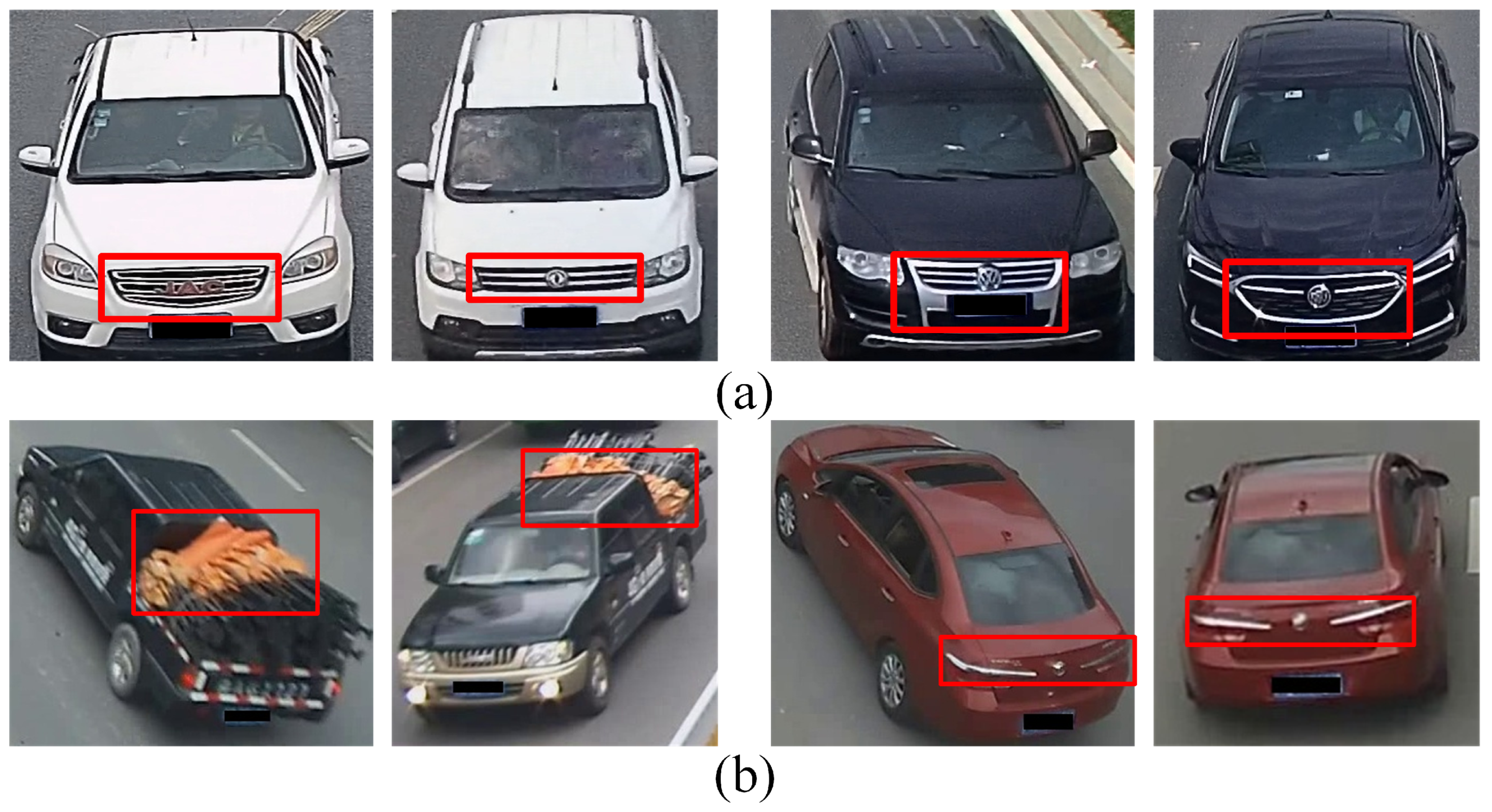
Figure 1. Two significant challenges in vehicle re-identification. (a) Different vehicles share a similar appearance. (b) The same vehicle exhibits different visual patterns, and the regions of key details are non-corresponding.
Applsci 14 03968 g001
Figure 2. The overall framework of our proposed approach. It consists of two streams. The top is the visual feature stream that employs an SaGT to extract global and stripe-based features for vehicle images. The lower left is the STPro stream that utilizes the location and timestamp of vehicles to estimate the probability when vehicles take time to move from one camera to another. The fusion module in the lower right fuses the global feature distance and the STPro for vehicle re-identification. (Best viewed in color.)
Applsci 14 03968 g002
Figure 3. Re-identification visualization examples on VeRi-776. For each query, the three rows from top to bottom show the top-10 retrieval results produced by Baseline, SaGT, and SaGT-ST, respectively.
Applsci 14 03968 g003
Figure 4. The Grad-CAM visualization of attention maps. The first, second, and third rows show the original image, Baseline, and SaGT, respectively.
Applsci 14 03968 g004
Table 1. The performance (%) comparison on VeRi-776. The best performance is marked in bold.
MethodTypeReferencemAPRank-1
SN [13]GFTNNLS’2275.7095.10
VARID [12]GFTITS’2279.3096.00
VAT [18]GFIPM’2280.4097.50
MsKAT [32]GFTITS’2282.0097.10
PGAN [15]LFTITS’2279.3096.50
DGPM [14]LFTITS’2179.3996.19
LG-CoT [36]LFICTAI’2279.7097.00
HPGN [37]LFTITS’2280.1896.72
DFR [38]LFPR’2284.4793.02
DSN [39]LFPR’2376.3094.80
SFMNet [40]LFIJCNN’2380.0097.00
GiT [31]LFTIP’2380.3496.86
SOFCT [22]LFTITS’2380.7096.60
MART [41]LFTITS’2382.7097.60
DPGM-ST [14]LF and STTITS’2182.1798.45
DFR-ST [38]LF and STPR’2286.0095.67
BaselineGFOurs78.3895.71
SaGTGFOurs80.6796.96
SaGT-STGF and STOurs86.5998.75
Table 2. The performance (%) comparison on VehicleID. The best performance is marked in bold.
MethodTypeReferenceSmallMediumLarge
mAPRank-1mAPRank-1mAPRank-1
SN [13]GFTNNLS’2278.8076.7076.8074.8076.3073.90
VARID [12]GFTITS’2288.5085.8084.7081.2082.4079.50
VAT [18]GFIPM’2289.9084.5087.1080.5085.0078.20
MsKAT [32]GFTITS’22-86.30-81.80-79.40
DFR  [38]LFPR’2287.5582.1584.9479.3383.1877.93
HPGN [37]LFTITS’2289.6083.9186.1679.9783.6077.32
PGAN [15]LFTITS’22----83.9077.80
LG-CoT [36]LFICTAI’2290.5085.2086.6080.5084.4078.00
DSN [39]LFPR’2381.7080.6079.1078.2075.5075.00
SOFCT [22]LFTITS’2389.8084.5086.4080.9084.3078.70
GiT [31]LFTIP’2390.1284.6586.7780.5284.2677.94
SFMNet [40]LFIJCNN’23-85.10-80.50-77.60
BaselineGFOurs85.0677.3881.6374.1378.0469.75
SaGTGFOurs91.3686.3387.3081.4484.3878.13
Table 3. The ablation study (%) of STPro on VeRi-776.
MethodFusionmAPRank-1
Baseline-78.3895.71
Baseline-STAdd82.94 (+4.56 )98.27 (+2.56)
Baseline-STMultiply84.93 (+6.55)98.75 (+3.04)
SaGT-80.6796.96
SaGT-STAdd84.61 (+3.94)98.33 (+1.37)
SaGT-STMultiply86.59 (+5.92)98.75 (+1.79)
Table 4. The ablation study (%) of SFM and SaGL on VeRi-776 and VehicleID. The best performance is marked in bold.
MethodVeRi-776VehicleID
SmallMediumLarge
mAPRank-1mAPRank-1mAPRank-1mAPRank-1
Baseline78.3895.7185.0677.3881.6374.1378.0469.75
SaGT-SFM80.3096.9689.6684.0086.0180.0983.8477.67
SaGT80.6796.9691.3686.3387.3081.4484.3878.13
Table 5. The performance of different features for inference on VeRi-776.
MethodFeaturemAP ↑Parameter ↓Time ↓Storage ↓
(%)(M)(ms/Image)(KB/Image)
SaGT-SFMGF80.3085.68.136
LF80.3385.713.4548
GF and LF80.3492.715.1754
SaGTGF80.6785.68.136
Disclaimer/Publisher’s Note: The statements, opinions and data contained in all publications are solely those of the individual author(s) and contributor(s) and not of MDPI and/or the editor(s). MDPI and/or the editor(s) disclaim responsibility for any injury to people or property resulting from any ideas, methods, instructions or products referred to in the content.