Abstract
This article presents an analysis of three different approaches to the identification of the thickness of the fouling layer inside the pipes of natural gas (NG) coolers. At present, there is no existing simple analytical procedure for the identification of the fouling layer thickness. The authors of this article describe in detail the balance method, which required the use of a large number of physical parameters, changes in their sizes depending on the output temperature of the gas, the temperature of the cooling air, the air quantity, as well as the physical properties of both media. The computational model was robust, and its disadvantage was the iterative computation. The second analysed method was a dimensional analysis. It was applied using the Buckingham’s theorem to express the individual similarity criteria. In this method, 10 simplexes and two complexes were created. The fouling layer thickness, expressed using a derived criterial equation, exhibited real results. The third analysed method was based on analysing selected physical parameters with the use of a multiple regression analysis in MinitabX 18 software. The analysis showed that the fouling layer thickness depended on fewer parameters than the number of parameters assumed in the dimensional analysis or the balance method. The standard deviation that was identified in the multiple linear regression for a double crossflow cooler was 0.0667 and the value of reliability (the coefficient of determination of the multiple linear regression) R2 was 0.9985.
1. Introduction
Natural gas coolers are pressure vessels with many thousands of sealed holes. In the coolers, cooled natural gas flows through tubes with external fins. The maximum projected gas pressure in coolers of various designs is 7.85 MPa. During the cooler operation, a fouling layer is formed on the inside wall of the tubes, and it reduces the cross-sectional area of the tubes. As the fouling layer thickness increases, several negative effects occur: a higher speed of the flowing gas, higher thermal resistance of the tube wall, changes in the operating conditions, etc.
The motivation for conducting the study presented in this article was to find a simple procedure that would facilitate the identification of the thickness of a fouling layer formed on a heat-transfer surface from any material whatsoever. Such materials may include, for example, a limescale layer inside the pipes of a heat exchanger, sediments on the walls of a plate heat exchanger in the pasteurisation of soy milk, and so forth. The currently available literature only provides general equations describing the cooling process for technical devices that require extensive iteration procedures. The authors of the present article have developed a simpler procedure that facilitates the identification of a real thickness of the fouling layer formed on the internal heat-transfer surfaces in the pipes of a cooler. Therefore, this study includes a rather detailed analysis of mathematical equations. The proposed method brings relevant results that have been validated in experiments.
Natural gas coolers are characterised by cooling surfaces of various sizes and shapes. The numbers of tubes and their arrangements inside the cooler block, as well as the methods of transporting gas through the tubes, may vary. Over a prolonged operation of a cooler, its cooling capacity decreases due to sediments accumulated on the internal and external surfaces of the tubes. Keeping the external heat-transfer surface clean is relatively easy; however, cleaning the internal surfaces is a complicated process. The cooler must be dismantled, all its tubes must be cleaned with the use of special technology, and then it must be re-assembled. As the cleaning technology is complicated and very long, the cooler must be removed from service for a long period of time; this causes a considerable financial loss to the gas transporter.
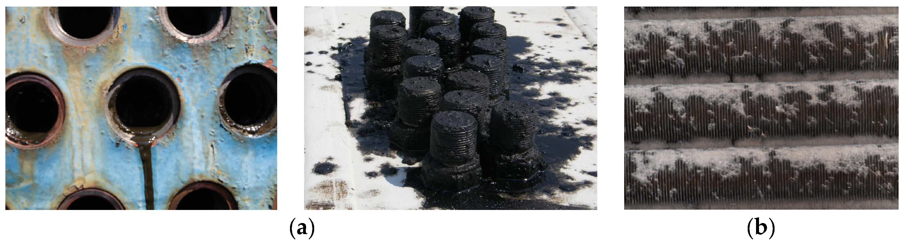
The currently available analytical procedures for the identification of a cooling capacity of any equipment in which heat is transferred between the cooled medium and the cooling medium are rather complicated. In general, the key challenge is to exactly identify the heat transfer coefficient for both the cooled medium and the cooling medium, especially in cases where the internal or external heat-transfer surfaces are fouled and the external surface has a complex shape. Figure 1 shows the real condition of a natural gas cooler fouled with impurities of an unknown composition. The authors of paper [1] identified the heat-transfer coefficient of the fouling layer in an experiment. Expressing a cooling capacity is also difficult due to the fact that the temperatures of the cooled medium and of the cooling medium change on the heat-transfer surface along the entire tube length [2,3,4]. The basics of the process of cooling gas media by applying ventilation technology may be found in the literature [5,6]. The analysed cooler was designed with the tubes arranged in several rows on top of each other. In each row, the temperatures of the gas and of the cooling air are different. As the temperatures change, the heat transfer coefficients for the internal and external sides also change, and so does the gas density and viscosity, as well as the thermal conductivity coefficient.

Figure 1.
Fouled tubes of the natural gas cooler (a); impurities on the external side of the fins (b).
The authors were searching for a procedure that would describe in the simplest possible way, but with sufficient accuracy, the process of formation of the fouling layer in natural gas coolers that are used in various compressor stations and have various shapes of the heat-transfer surface. In this article, two different methods for the identification of the fouling layer thickness were analysed: the balance method, and the procedure using dimensional analysis. When applying dimensional analysis, it is advisable to confront the obtained results with the results obtained by a physical experiment [7] or numerical modelling [8,9], or a complicated analytical procedure [10,11,12]. The method that is described in this article is based on the basics of the probability theory and modelling presented in papers [13,14,15,16,17,18]. Dimensional analysis was also applied in papers [19,20].
The authors of this article have published their own studies on the application of dimensional analysis in various fields in relevant journal studies and publications. A summary of the modelling methods applied with the use of dimensional analysis is presented in publication [21].
For the purpose of proving the applicability of the created mathematical model, the task presented in this article was carried out with a double crossflow cooler. Such coolers are used in compressor stations, for example in Veľké Kapušany, Veľké Zlievce, and elsewhere in Slovakia, as well as in other countries.
Each of the aforesaid methods is described in detail in Section 2.
2. Mathematical Models for Expressing the Fouling Layer Thickness
Each of the methods described below has its positive and negative sides. It is important that the used method is as simple as possible in expressing the fouling layer thickness and provides real results compared to the complicated procedures. In this study, the experimental verification of results was not acceptable for the reasons mentioned in the introductory and final sections of this article. Therefore, the comparison will involve the results obtained by applying the individual methods described below.
2.1. Balance Method
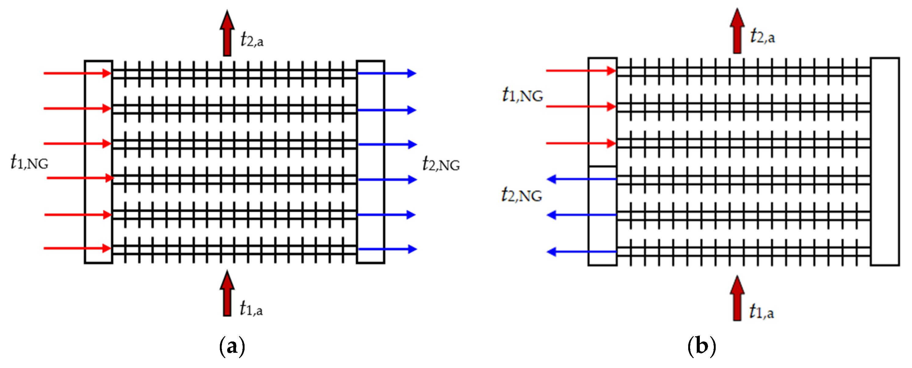
The balance method is based on a comparison of the supplied and removed heat output using Equation (1). The method applicable to a crossflow cooler (Figure 2a) is described in detail in paper [1], while the results related to a double crossflow cooler (Figure 2b) are presented in this article.
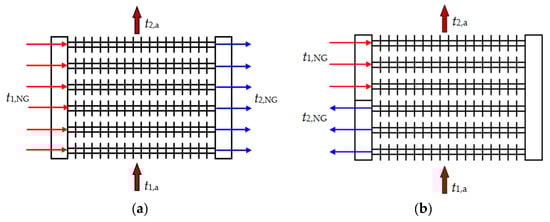
Figure 2.
Tube arrangement in the cooler block: (a) crossflow; (b) double crossflow.
The equation for calculating the cooling capacity P is as follows:
wherein P1 is the heat output withdrawn from natural gas (W); ηlos is the coefficient respecting the heat loss into the cooler’s structure (1); Qm,NG or Qm,a is the mass flow rate of gas or air flowing through the cooler (kg∙s−1); i1,NG, i2,NG is the specific enthalpy of gas at the entry into and exit from the cooler (J∙kg−1); and i1,a, i2,a is the specific enthalpy of air at the entry into and exit from the cooler (J∙kg−1).
Assuming that, for example, 3% of the output P1 transfers into the cooler’s structure, then coefficient ηlos equals 0.97 and the following equation is applied:
Concurrently with Equation (1), the following equation is applied:
wherein k is the overall heat transfer coefficient (W·m−2·K−1); is the mean temperature gradient (K); and SΣ is the total heat-transfer surface area of the cooler (m2).
The total surface area of the cooler SΣ in Equation (3) is determined by the product of the external surface area of a single tube Se (m2) and the number of all tubes in the cooler np:
The surface area of a single tube is calculated using the following equation:
wherein r is the number of fins on a single tube (1); dr is the fin diameter (m); d2 is the external diameter of the tube (m); and b is the fin spacing (m).
The mean temperature gradient (K) in Equation (3) may be identified using the equations presented in detail in paper [1]. The analysed cooler used a double crossflow with two flow runs n = 2. The correction coefficient ψ that is necessary for the identification of the mean temperature gradient is therefore calculated using the following equation:
For parameter A, the Equation (6) determines the following:
The P and R criteria are identified using the following equations:
wherein KNG is the heat capacity rate of gas; Ka is the heat capacity rate of air (W·K-1).
The heat capacity rate expresses the output that is required to heat the mass of the flowing medium by 1 K and is calculated using the following equation:
wherein cp is the specific heat capacity of the medium (J∙kg−1∙K−1).
After substituting the total heat-transfer surface area and the mean temperature gradient into Equation (3), the overall heat transfer coefficient k may be calculated using Equation (10):
Coefficient k may also be calculated based on a detailed description of the process of heat transport from warm natural gas through the tube wall into the surrounding air. If there is a fouling layer inside the tube, the solution must also take into account the heat transfer through that fouling layer.
The authors of this article assumed that the cooler had a fouling layer inside and a clean external heat-transfer surface, and they derived the following equation for calculating the overall heat transfer coefficient:
wherein α1 is the coefficient of heat transfer inside the tube (W∙m−2∙K−1); hf is the thickness of the fouling layer in the tube (m); λf is the thermal conductivity coefficient of the fouling layer (W∙m−1∙K−1); λp is the thermal conductivity coefficient of the tube (W∙m−1∙K−1); S1 is the internal surface area of the tube (m2); d1 is the internal diameter of the tube (m); sp is the thickness of the tube wall; L is the tube length (m); and α2 is the heat transfer coefficient for the heat transfer from the finned tube into the air (W∙m−2∙K−1).
By comparing Equations (11) and (10), the following equation for calculating the fouling layer thickness was obtained:
Parameter D in Equation (12) was as follows:
The key challenge associated with calculating the fouling layer thickness using Equation (12) was that some of the parameters in Equation (12) are a function of hf. As hf increases, the thermal resistance on the tube wall also increases, and this leads to a decrease in the cooling capacity P. The fouling layer reduces the internal diameter of the tube and, consequently, the natural gas flow rate increases as well as the value of coefficient α1. The heat transfer coefficient α1 is calculated using a criterial equation that contains, inter alia, the Reynolds number Re. A higher α1 value leads to a lower value of thermal resistance on the interface between the natural gas and the internal wall of the tube. As a result, the cooling capacity increases. Moreover, changes in the fouling layer thickness cause changes in the mean temperature gradient . Based on the aforementioned facts, it may be stated that the fouling layer thickness cannot be calculated directly and requires numerous iterations.
The basic geometric parameters of the analysed cooler are listed in Table 1.

Table 1.
Geometric parameters of the analysed cooler.
The efficiency of the gas cooling process is significantly affected by the thermal conductivity of the fouling layer. The authors of this article identified the thermal conductivity coefficient of the fouling layer in an experiment. The coefficient value was 0.746 W·m−1·K−1, approximately two orders lower than the value for the tube material [1].
The key settings for the iterations were selected based on the project values of the cooler’s parameters. The cooler was designed to cool natural gas at 242.3 kg·s−1 and a pressure of 7.45 MPa from a temperature of 75 °C to 50 °C. The required quantity of the fan air with a temperature of 28 °C was 565.23 kg·s−1.
In the project, it was assumed that the heat-transfer surfaces were clean; therefore, hj = 0 was substituted into Equation (11). A similar procedure was applied to the iterations that were used for the temperatures of the cooling air which were different from the projected temperature. The ambient temperature ranged from 28 to 0 °C. The mass flow rate, the input temperature, and the gas pressure remained constant during the process. As the ambient temperature decreased, the amount of the air decreased, as described by the following equation:
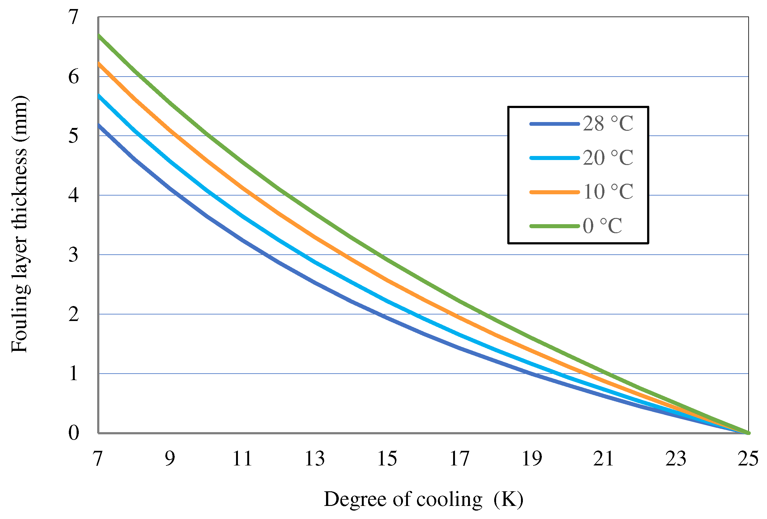
Selected results of iterations are presented in Figure 3. For certain values of the ambient temperature, the curve of the fouling layer thickness corresponds to the relevant gas cooling degree.
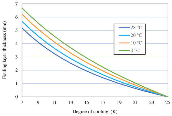
Figure 3.
Correlation between the gas cooling degree and the fouling layer thickness for selected ambient temperatures.
The indicated calculation method is rather complicated. Moreover, it requires obtaining extensive input data before the solving process is commenced—not only geometric data, but also the values of physical properties of natural gas and air. Particularly in the case of natural gas, with a pressure ranging from approximately 6 to 7.5 MPa, complex functions that depend on a pressure and a temperature must be applied in order to describe its physical properties.
Due to the complexity of the iteration procedure, the authors attempted to identify the fouling layer thickness through dimensional analysis based on the Buckingham’s theorem.
2.2. Buckingham’s Method
In the first approximation, all the parameters that were selected for the purpose of deriving a criterial equation were identical to those used in the balance method. In addition to the parameters listed above, these also included density, the thermal conductivity coefficient and kinematic viscosity of the flowing media, as well as the thermal conductivity coefficients of the tube and fin materials. A total of 18 dimensionless criteria were created and the criterial equation was subjected to an analysis, which revealed the effects of the individual criteria on the resulting hf value. The parameters with apparently minor effects were then withdrawn from the model, and a new, simpler model was created. In the new model, some of the geometric dimensions (e.g., the external diameter of the tube, the fin diameter and thickness, and the fin spacing) were replaced with the surface areas calculated on the basis of those parameters. The adjusted list of physical parameters (16 in total) is presented in Table 2.
Table 2.
Input parameters for the mathematical model.
In the creation of the model law, all the dimensions of the selected physical parameters were transformed into seven SI base units (kg; m; s; K, A; mol; cd). The relevant parameters in the aforesaid model for the identification of the fouling layer thickness included only four basic dimensions—kg, m, s, and K.
A criterial equation is normally created by replacing the selected dimensional parameters φ1 through φn with similarity criteria π1 through πm, while the functional correlations between the individual criteria are identified experimentally or through numerical or analytical calculations. The resulting criterial equation then applies to the entire group of similar processes.
When a dimensional analysis is used to describe a process, the number of obtained criteria π is always lower than the number of relevant parameters n on which the process depends. The basic equation that expresses the corelations between n relevant parameters φ1, φ2 … φi … φn of various dimensions is as follows [21]:
Based on the defining equation, each of the φ parameters may be expressed through a specific dimensional equation. It is the product of the base unit symbols with the respective exponents. For the four base units of the selected physical parameters (kg, m, s, K), the defining equation is as follows:
In Equation (16), dimensional exponents x1 through x4 are rational numbers that were identified as described below.
Equation (15) is dimensionally homogenous; therefore, φi variables cannot be used separately, but only in the form of products:
wherein
- π—is the dimensionless variable (similarity criterion) (1);
- xi—is the exponent (rational number);
- φi—is the physical parameter with a respective dimension.
Pursuant to Equation (15) and considering the physical parameters listed in Table 2, the following correlation must apply:
In general, for a certain phenomenon that is described by n relevant parameters, it is possible to create l similarity criteria. The number of searched criteria π is identified using the following equation:
wherein h is the je rank of the dimension matrix.
Pursuant to Equation (17), the following applies:
The dimensional form of Equation (20) is as follows:
Since the left side of Equation (21) equals one, the sum of the dimensional exponents in every basic parameter must equal zero. Therefore, the individual dimensions of the physical parameters (kg, m, s, K) are subject to the set of Equations (22)–(25).
For the “kilogram” unit:
For the “meter” unit:
For the “second” unit:
For the “Kelvin” unit:
The rank of the matrix for the set of Equations (22)–(25) equals four. With a total of 16 physical parameters, the total number of criteria is l = 12, as calculated using Equation (19).
Parameters with identical dimensions are expressed as independent criteria, also referred to as simplexes. The number of simplexes ls equals the difference between the total number of relevant parameters n and the number of relevant parameters with different dimensions nk; therefore:
Table 1 indicates that the number of parameters with different dimensions is six. This means that a task with 16 relevant parameters may be assigned 10 simplex criteria.
The simplex that was created on the basis of the heat capacity rate values, calculated for gas and air using Equation (9), is as follows:
The temperature simplex criteria are as follows:
The simplexes created from the parameters with a length dimension are as follows:
The fouling layer is affected by the flow surface area; therefore, the following simplex was created:
The simplex created from the gas and air density parameters is as follows:
The simplex for the thermal conductivity coefficients for the gas and for the fouling layer is as follows:
With regard to the created simplexes, in the set of Equations (22)–(25), x2 = x3 = x5 = x8 = x9 = x10 = x11 = x12 = x14 = x16 = 0; therefore, the resulting equations are as follows:
The total number of searched criteria is l = 12 and the number of created simplexes is 10. The two missing complex criteria had to be identified based on two independent solutions of the set of Equations (37)–(40).
The set of Equations (37)–(40) contains six unknowns; therefore, they must be solved by determining two of those unknowns and calculating the remaining four.
In the first option, the determined unknowns were x1 = 1 and x6 = 0 and the calculated parameters were the following: x4 = 0; x7 = −1; x13 = 0; and x15 = −1. The identified criterion was as follows:
In the second option, the determined unknowns were x6 = 1 and x1 = 0 and the calculated parameters were the following: x4 = 0; x7 = −2; x13 = 0; and x15 = 0. The identified criterion was as follows:
Since the criterial equation was to be derived for a particular cooler, the criteria π4, π5, π6, π7, and π12 were constant. Therefore, they were pooled into a single new criterion π0.
As a rule, similarity criteria may be transformed into other criteria through multiplication, division, exponentiation with a constant, or multiplication by a constant [21]. That rule was applied to obtain the following new criterion from the constant criteria:
The parameter that was being identified was the thickness of the fouling layer in the cooler tubes hf, and since it fell within the π8 criterion, it was expressed as a function of other criteria, with the following form:
The correlation between the dimensionless arguments in Equation (44) is exponential; therefore, the resulting equation is as follows:
In a logarithmic scale, that correlation is linear and in the following form:
The individual criteria were calculated from the parameter values that were identified through iterations as described above. For the multiple regression analysis, data from 94 iterations were available. The C constant and the unknown exponents zj were identified through multiple linear regression.
The coefficient of determination for the multiple linear regression was 0.9999. The regression sum of squares was 13.153, while the residual sum of squares was 0.005. The values of the C constant and the individual exponents are listed in Table 3.
Table 3.
C constant and the individual exponents.
For the analysed cooler, the thickness of the fouling layer in the cooler tubes was subjected to the following criterial Equation (47), obtained by breaking down Equation (45):
Criteria with a zero exponent were not specified in Equation (47). In the linear regression, their impact was automatically included in the value of the C constant.
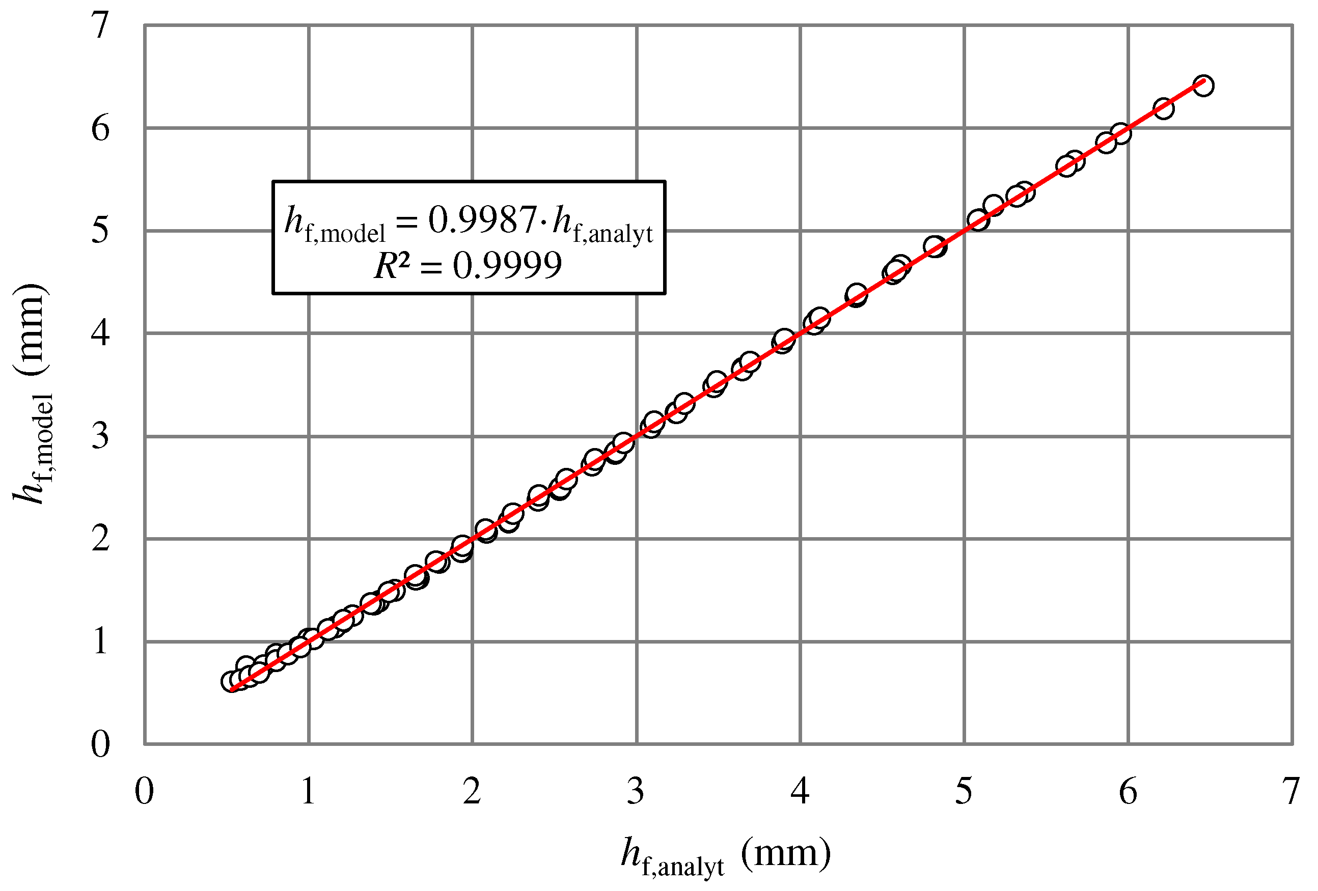
The parameter that was being identified—the fouling layer thickness hf—is on the left side of criterial Equation (47) and is affected by the internal diameter of the cooler tube d1. An adjustment of this criterion leads to solving a quadratic equation. Only one of the identified roots of the equation had a physical meaning—the one with a lower value. The values of the fouling layer thickness obtained from the model and from the analytical solution exhibited very good concordance (Figure 4).
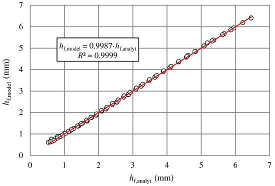
Figure 4.
Correlation between the fouling layer thickness obtained from the analytical solution and the thickness obtained from the model created by applying the Buckingham’s theorem.
The correlation may be described by a regression line with a slope approaching 1, more specifically 0.9987, with a reliability value (a squared correlation index) R2 = 0.9999. The standard deviation of the difference was 0.0331, i.e., 3.2%.
The results of both solutions were also subjected to a pairwise t-test at a significance level α = 0.05. A precondition for using a pairwise t-test was meeting the assumption of normality of the difference scores, which was verified in a Shapiro–Wilk test of normality. The value of the test criterion t was identified using the following equation:
wherein m is the number of values (1) and sΔ is the standard deviation (mm).
Parameter is the average value of the difference Δhf,analyt,i − Δhf,mod,i, calculated using the following equation:
For the analysed data sets, m = 94 and mm; therefore, the value of the test criterion t was 0.030. The critical value tcr at a significance level of 0.05 was t0.05(94−1) = 1.986. Since t < tcr, it may be stated that both methodologies provided identical results.
2.3. Multiple Regression Analysis
In a general case, the derived Equation (47) describes the fouling layer thickness with sufficient accuracy. However, the model is not very convenient for common purposes as it includes 12 independent parameters. Therefore, the investigation was carried out with the aim of exploring how to reduce the number of relevant parameters. In any cooler, the individual criteria of Equation (47) contain certain parameters that are of a constant value. In the analysed cooler, those parameters included, for example, the thermal conductivity coefficient for the pipe material and the fouling layer, the internal and external diameters of the pipe, the pipe lengths, etc.
In this case, the fouling layer thickness was identified by applying multiple regression analysis, using the MinitabX 18 statistical software and the R package software 4.3.3 [22].
With the use of MinitabX, out of the group of relevant parameters, the following six parameters were selected as those with the most significant impact on the fouling layer thickness: Qm,a; T2,NG; T1,a; ρNG; ρa; and cp,NG. Multiple linear regression was applied and the following model equation was created:
Gas density ρNG was used in Equation (50) for the mean temperature value (T1,NG − T2,NG)/2, and it was identified using Equation (51):
Air density ρa was calculated using Equation (52):
wherein .
The specific thermal capacity of gas cp,NG was calculated using Equation (53):
Equation (50) represents the model of a correlation between the fouling layer thickness and the selected input parameters. The regression model parameters were identified by applying the method of least squares, which is sensitive to outliers. Therefore, the input data was also assessed in terms of outliers and influential values, which were excluded from the model.
The statistical significance of the regression model, or of the regression model parameters, was verified in the tests of statistical significance at a significance level α = 0.05. As a rule, if the p-value is lower than the significance level α, then the null hypothesis is rejected in favour of the alternative hypothesis. If the p-value equals or is higher than the selected significance level α, then the null hypothesis is not rejected [23]. The results of the testing showed that the regression model (50) was statistically significant (p-value = 3 × 10−122 < α) and that all of the analysed parameters were also statistically significant (p-value < α). The coefficient of determination for the multiple linear regression was 0.9985; this means that as much as 99.85% of the fouling layer thickness variability may be explained by the proposed regression model with the given parameters.
Heteroscedasticity of the regression model was tested with the use of the Breusch–Pagan test, in which the null hypothesis assumes homoscedasticity. The results (p-value = 0.199 > α) indicated that the regression model did not exhibit heteroscedasticity.
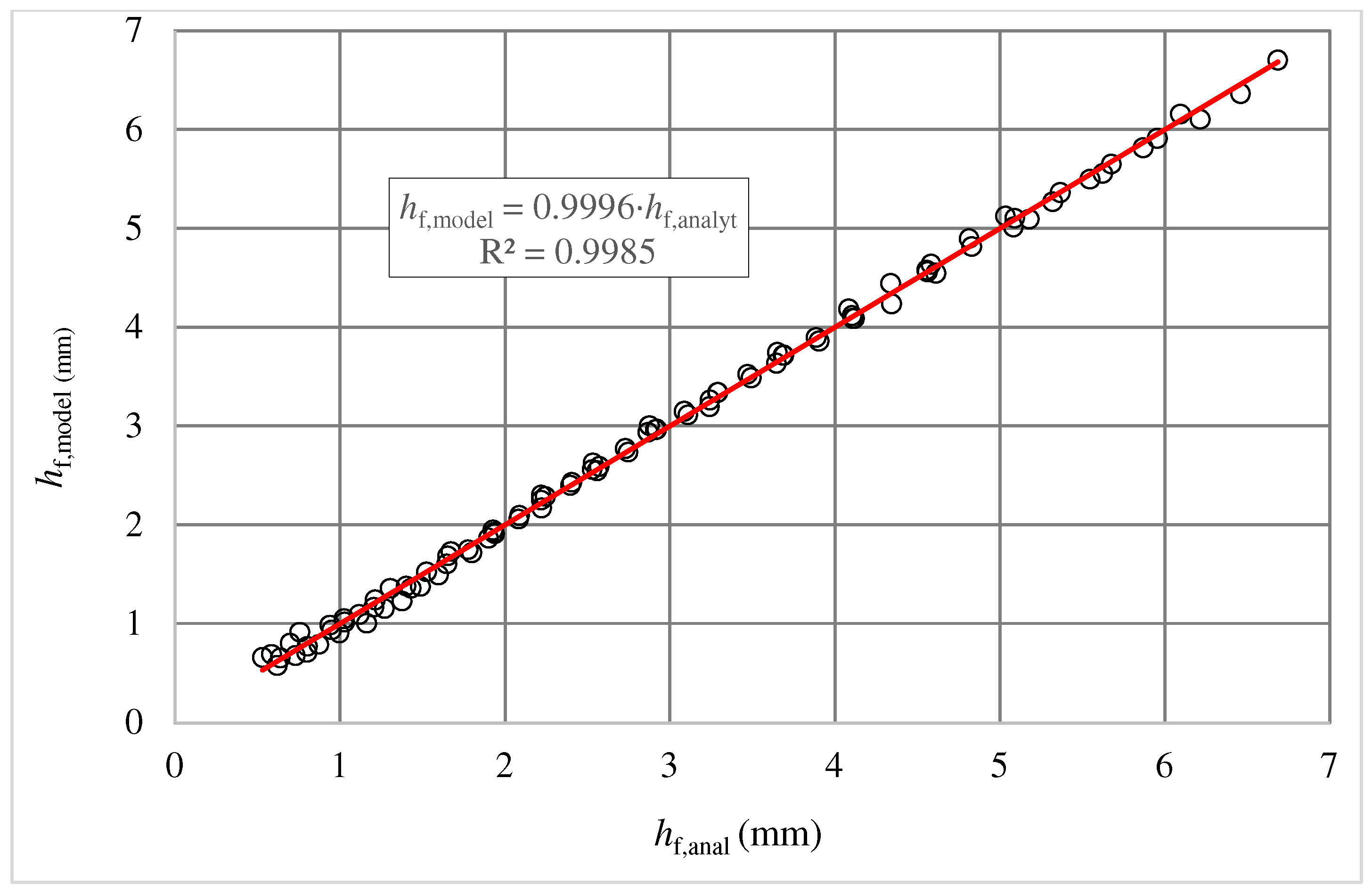
The correlation between the fouling layer thickness obtained from the model created by applying the multiple regression and that obtained analytically may be described by a regression line (Figure 5) with a slope approaching 1, in particular 0.9996, at a reliability value R2 = 0.9985.
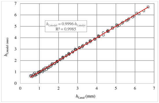
Figure 5.
Correlation between the fouling layer thickness obtained analytically and the fouling layer thickness obtained from the model created through multiple regression.
The values of the fouling layer thickness obtained from the model and from the analytical solution were compared in a pairwise t-test at a significance level α = 0.05. The Shapiro–Wilk test of normality was used to verify data normality. The results of the pairwise t-test (p-value = 0.999 > α) indicated that the two methodologies provided comparable results. The tests were performed using the R package software [24].
3. Conclusions
Based on the performed analyses, it may be stated that the application of the balance method and dimensional analysis to the processes that are affected by a relatively large number of relevant parameters is not very beneficial. It is more appropriate to describe such processes with the use of a regression equation constructed from selected parameters, and not from similarity criteria.
The constructed regression Equation (50) is simple and easy to use for a double crossflow cooler of natural gas. It is therefore unnecessary to put the cooler out of service and dismantle the tubes inside the cooler in order to examine the extent of the fouling layer accumulated on the surface inside the tubes. Such interruptions in the cooler operation cause severe outages in the cooling process and result in a considerable financial loss associated with an interruption in the transportation of gas, as well as the dismantling and re-assembly of the cooler tubes, because there are thousands of tubes in a cooler.
Equation (50) was validated during the process of cleaning the analysed cooler. Prior to the cleaning, the gas temperature at the outlet from the cooler was 15 K lower than the temperature at the inlet. The temperature of the surrounding air was 20 °C. Based on the volume of the fouling matter that was pushed out of all the pipes in the cooler, the average thickness of the fouling layer on the inner pipe surface was calculated as 2.22 mm. The thickness of the fouling layer calculated using Equation (50) was 2.15 mm. The difference between the two values represents 3.1%.
Equation (50) may be simply programmed, and in case of a change in the gas output temperature and the ambient temperature, it facilitates identifying the current thickness of the fouling layer on the internal surface of the cooler tubes without the need to put the entire cooler out of service.
The presented methodology may be applied at any compressor station in Slovakia, as well as any other country, where natural gas is cooled by coolers of the same design as the design of the cooler subjected to the analysis described in this article.
Author Contributions
Conceptualization, M.Č., M.P., M.A. and L.T.; formal analysis, M.Č. and L.T.; visualization, M.Č. and L.T.; validation, M.P, M.Č. and M.A. All authors have read and agreed to the published version of the manuscript.
Funding
This paper was written with the financial support from the VEGA granting agency within the Projects No. 1/0224/23 and No. 1/0532/22, from the KEGA granting agency within the Project No. 012TUKE-4/2022, and with the financial support from the APVV granting agency within the Projects No. APVV-15-0202, APVV-20-0205, and APVV-21-0274, and project SP 2024/025-FMT VŠB TUO.
Institutional Review Board Statement
Not applicable.
Informed Consent Statement
Not applicable.
Data Availability Statement
Data is contained within the article.
Conflicts of Interest
The authors declare no conflicts of interest.
References
- Čarnogurská, M.; Příhoda, M.; Molínek, J. Determination of deposit thickness in natural gas cooler based on the measurements of gas cooling degree. J. Mech. Sci. Technol. 2011, 25, 2935–2941. [Google Scholar] [CrossRef]
- Spalding, D. Heat Exchanger Design Handbook: Heat Exchanger Theory; VDI-Verlag GmbH: Düsseldorf, Germany, 1983; p. 2305. [Google Scholar]
- Dekebo, S.B.; Oh, G.-T.; Lee, M.-W. Cleaning Schedule Optimization of Heat Exchanger Network Using Moving Window Decision-Making Algorithm. Appl. Sci. 2023, 13, 604. [Google Scholar] [CrossRef]
- Lyons, W.C.; Plisga, G.J.; Lorenz, M.D. Standard Handbook of Petroleum and Natural Gas Engineering, 3rd ed.; Elsevier: Amsterdam, The Netherlands, 2016; ISBN 978-0-12-383846-9. [Google Scholar]
- Sekulic, D.P.; Shah, R.K. Fundamentals of Heat Exchanger Design; John Wiley and Sons Ltd.: Hoboken, NJ, USA, 2023; p. 800. [Google Scholar]
- Nemati, N.; Ardekani, M.M.; Mahootchi, J.; Meyer, J.P. Fundamentals of Industrial Heat Exchangers; Selection: Design, Construction, and Operation; Elsevier—Health Sciences Division: Amsterdam, The Netherlands, 2024; p. 514. [Google Scholar]
- Gullberg, P.; Sengupta, R.; Horrigan, K. Transient fan modelling and effects of blade deformation in a truck cooling fan installation. In Proceedings of the Vehicle Thermal Management Systems Conference Proceedings (VTMS11), Coventry, UK, 15–16 May 2013; pp. 219–227. [Google Scholar] [CrossRef]
- Brestovič, T.; Čarnogurská, M.; Příhoda, M.; Lukáč, P.; Lázár, M.; Jasminská, N.; Dobáková, R. Diagnostics of Hydrogen-Containing Mixture Compression by a Two-Stage Piston Compressor with Cooling Demand Prediction. Appl. Sci. 2018, 8, 625. [Google Scholar] [CrossRef]
- Puškár, M.; Brestovič, T.; Jasminská, N. Numerical simulation and experimental analysis of acoustic wave influences on brake mean effective pressure in thrust-ejector inlet pipe of combustion engine. Int. J. Veh. Des. 2015, 67, 63–76. [Google Scholar] [CrossRef]
- Li, H.; Ding, X.; Jing, D.; Xiong, M.; Meng, F. Experimental and numerical investigation of liquid-cooled heat sinks designed by topology optimization. Int. J. Therm. Sci. 2019, 146, 106065. [Google Scholar] [CrossRef]
- Ting, D. Thermofluid: From Nature to Engineering, 1st ed.; Elsevier, Academic Press: Amsterdam, The Netherlands, 2022; p. 434. [Google Scholar]
- Jirouš, F. Application of Heat and Mass Transfer; CVUT Praha: Prague, Czech Republic, 2010; p. 207. (In Czech) [Google Scholar]
- Sritham, E.; Nunak, N.; Ongwongsakul, E.; Chaishome, J.; Schleining, G.; Suesut, T. Development of Mathematical Model to Predict Soymilk Fouling Deposit Mass on Heat Transfer Surfaces Using Dimensional Analysis. Computation 2023, 11, 83. [Google Scholar] [CrossRef]
- Langhar, H.L. Dimensional Analysis and Theory of Models; Kreiger Publishing Company: Malabar, FL, USA, 1987; p. 166. [Google Scholar]
- Barenblatt, G.I. Dimensional Analysis; Gordon and Breach Science Publishers: New York, NY, USA; London, UK; Paris, France; Montreaux, Switzerland; Tokyo, Japan, 1987. [Google Scholar]
- Görtler, H. Dimensionsanalyse: Theorie der Physikalischen Dimensionen mit Anwendungen; Springer: Berlin/Heidelberg, Germany, 1975. (in German) [Google Scholar]
- Kožešník, J. Similarity Theory and Modelling; Academia: Praha, Czech Republic, 1983. (In Czech) [Google Scholar]
- Huntley, H.E. Dimensional Analysis; Dover Publications: New York, NY, USA, 1967. [Google Scholar]
- Dumka, P.; Chauhan, R.; Singh, A.; Singh, G.; Mishra, D. Implementation of Buckingham’s Pi theorem using Python. Adv. Eng. Softw. 2022, 173, 103232. [Google Scholar] [CrossRef]
- Hongxian, Y.G.; Rong, X.F.; Paneiro, G. Ground-Borne Vibration Model in the near Field of Tunnel Blasting. Appl. Sci. 2023, 13, 87. [Google Scholar] [CrossRef]
- Čarnogurská, M.; Příhoda, M. Application of Dimensional Analysis for Modeling Phenomena in the Field of Energy; SjF TUKE: Košice, Slovak, 2011; pp. 113–129. (In Slovak) [Google Scholar]
- Keith, T.Z. Multiple Regression and Beyond: An Introduction to Multiple Regression and Structural Equation Modeling, 3rd ed.; Routledge: New York, NY, USA, 2019; 654p. [Google Scholar]
- Montgomery, D.C.; Runger, G.C. Applied Statistics and Probability for Engineers, 7th ed.; John Wiley & Sons: New York, NY, USA, 2018; 720p. [Google Scholar]
- Dalpiaz, D. Applied Statistics with R; GitHub Publisher: Champaign, IL, USA, 2021; 417p, Available online: https://book.stat420.org/ (accessed on 14 December 2023).
Disclaimer/Publisher’s Note: The statements, opinions and data contained in all publications are solely those of the individual author(s) and contributor(s) and not of MDPI and/or the editor(s). MDPI and/or the editor(s) disclaim responsibility for any injury to people or property resulting from any ideas, methods, instructions or products referred to in the content. |
© 2024 by the authors. Licensee MDPI, Basel, Switzerland. This article is an open access article distributed under the terms and conditions of the Creative Commons Attribution (CC BY) license (https://creativecommons.org/licenses/by/4.0/).