This section elucidates the SkinSwinViT methodology and presents the dermoscopic image dataset utilized for the classification of seven distinct lesion types.
3.3. Proposed SkinSwinViT Architecture
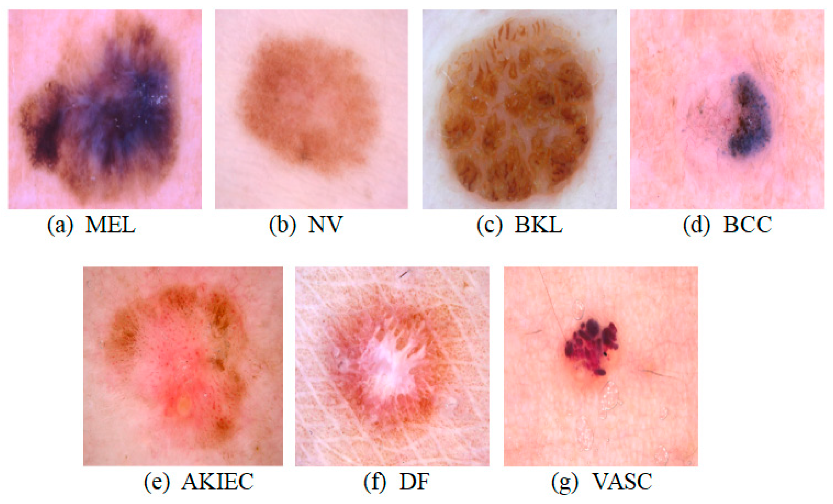
The SkinSwinViT model, as proposed in this study, is designed for the purpose of identifying skin disorders classified into seven distinct categories.
Figure 3 presents the architectural design of the SkinSwinViT model. Drawing inspiration from SwinViT [
32], the model primarily integrates components including data preprocessing, SwinTransformer Block, Global Attention Block, and Classifier Block.
To address the imbalance within the skin lesion dataset during data preprocessing, augmentation techniques are employed to enrich the segmented training set. Subsequently, the parameters of the pre-trained model serve as initial values. Following this, the proposed methodology utilizes a two-layer encoder, comprising SwinTransformer Block and Global Attention Block, to extract nuanced features across various dimensional spaces. Finally, the proposed method employs a Classifier Block to ascertain the categorical outcome of skin lesion images. The detailed framework is expounded below.
1. SwinTransformer Block: Derived from the SwinViT model, the SwinTransformer Block initially conducts patching to segment skin lesion images into smaller patches, facilitating localized processing and computational efficiency. Embedding preserves spatial relationships among patches, facilitating comprehensive feature capture. Subsequently, Windowed Multi-Head Self-Attention (W-MSA) and Shifted Windowed Multi-Head Self-Attention (SW-MSA) are employed to capture local features and inter-patch relationships. These attention mechanisms enable contextual comprehension of local information, enhancing feature extraction efficacy. By integrating W-MSA and SW-MSA, contextual dependencies between neighboring patches are effectively captured, bolstering feature extraction. Moreover, employing multiple Swin Blocks within the SwinTransformer Block facilitates the learning of complex, abstract-level features. Each Swin Block comprises layers of W-MSA and SW-MSA. Additionally, patch merging reduces image resolution and integrates multi-scale information, enhancing overall comprehension.
Specifically, the Patching and Embedding layer divides the input image
into non-overlapping patches of size 4 × 4, mapping dimensions to C dimensions to produce an embedded image
. Subsequently,
is normalized using Layer Normalization and forwarded to the Swin Block for feature extraction. The SwinTransformer Block consists of four stages, with patch merging operations at the conclusion of the first three stages to alter input feature dimensions. [1, 1, 3, 1] Swin Blocks are utilized across four stages, with channel counts per stage as [C, 2C, 4C, 8C]. The attention mechanism within each Swin Block is detailed as follows:
where
and
represent output features of W-MSA and Multi-Layer Perceptron (MLP) modules, respectively.
and
denote functions of W-MSA and SW-MSA, respectively.
represents the transformation function of the SwinTransformer Block.
2. Global Attention Block: Comprising multi-head self-attention mechanisms, layer normalization, and MLP layers, the Global Attention Block integrates spatial and semantic information. A multi-head self-attention mechanism fuses global information, followed by residual connections and layer normalization for feature representation learning. Subsequently, an MLP layer, comprising two linear layers and a nonlinear activation function (e.g., GELU), integrates feature information from different locations to generate a comprehensive global feature representation. This block enables global contextual comprehension through self-attention calculations on all feature vectors. The algorithm for the global attention mechanism is articulated as follows:
Here, represents the multi-head self-attention mechanism, are the query, key, and value matrices, respectively. is the dimensionality of the key vectors and is used to scale the dot product to prevent gradient vanishing or exploding. The Softmax function converts the dot product results into a probability distribution. signifies the concatenation of multi-head attention mechanisms. is a weight matrix, and is a bias term. denotes the transformation function of the Global Attention Block. denotes the residual connection. stands for Layer Normalization, which is used to stabilize the training process.
3. Classifier Block: Incorporated within the model decoder, the Classifier Block commences with layer normalization to stabilize data distribution and expedite training. Following normalization, the feature vector undergoes dimensionality reduction via adaptive average pooling to compress feature vector length from sequence length to a fixed length 1. This compression retains essential features, facilitating efficient data representation. The data then progresses to a linear transformation layer to learn input-output linear relationships. Ultimately, the linear layer output is processed through a Softmax function, yielding a probability distribution for final classification. This distribution reflects model confidence or likelihood for each class, enabling classification based on the highest probability class.
4. Loss Function: The model’s classification loss function utilizes cross-entropy loss, quantifying disparities between model-predicted probability distributions and true label distributions. The loss function is expressed as follows:
Here, L denotes the loss value, represents category j value in the true label (utilizing one-hot encoding), symbolizes model-predicted probability value for category j, N represents category count, and M represents sample count. The summation symbol accumulates all categories.
3.5. Performance Metrics
To evaluate the performance of individual models such as the proposed SkinSwinViT, this study considers the following performance metrics.
To measure the performance indicators of multi-classification, after data enhancement technology processing, the number of pictures in each category is the same, and there is no imbalance in the number of samples, so this paper adapts the Macro-average method. In multiclass classification problems, Macro-average calculates the indicators of each category and then averages the indicators of all categories. This is equivalent to setting the weights of all categories to be consistent. The specific formula is as follows:
represents the accuracy of prediction of a certain category among the seven categories of skin diseases. represents one of the seven types of skin diseases. The same applies to other indicators, where n represents the number of classification categories. In this article, n = 7, and the summation symbol is used to accumulate all categories. The indicators referred to in this study, by default, refer to the above-average indicators.
(True Positive): Refers to the number of instances that are correctly predicted to be a certain type of skin disease. (False Negative): Refers to the number of instances that are incorrectly predicted to be not a certain type of skin disease. (False Positive): Refers to the number of non-skin disease instances that are incorrectly predicted to be a certain type of skin disease. (True Negative): Refers to the number of cases of non-skin diseases that are correctly predicted to be non-skin diseases. Recall quantifies the frequency with which a classifier accurately predicts a positive outcome among all samples that should have been classified as positive. High precision indicates the test’s ability to precisely identify positive samples, thereby mitigating the occurrence of false positives. Elevated specificity signifies the accurate exclusion of negative samples and a diminished risk of misdiagnosis. The F1 score, as the harmonic mean of precision and recall, offers a comprehensive assessment of a classifier’s accuracy in predicting positive instances.
This study employs the ROC (Receiver Operating Characteristic) curve and AUC (Area Under the Curve) value for separate analyses of each category. The ROC curve plots the False Positive Rate (FPR) on the x-axis and sensitivity on the y-axis. Sensitivity measures the correct identification of positive examples, while the false positive rate represents the incorrect identification of negative examples. The formula for calculating the false positive rate is as follows:
The AUC is a metric that measures the overall performance of a classification model by calculating the area under the ROC curve. A higher AUC indicates better classification effectiveness for the model. The AUC value typically falls between 0.5 and 1.0, where 0.5 represents a random classifier, and 1.0 represents a perfect classifier.


