Article

Research on Multi-Objective Flexible Job Shop Scheduling Problem with Setup and Handling Based on an Improved Shuffled Frog Leaping Algorithm

School of Modern Post (School of Automation), Beijing University of Posts and Telecommunications, Beijing 100876, China
*
Author to whom correspondence should be addressed.
Appl. Sci. 2024, 14(10), 4029; https://doi.org/10.3390/app14104029
Submission received: 3 April 2024 / Revised: 30 April 2024 / Accepted: 7 May 2024 / Published: 9 May 2024

Abstract

:
Flexible job shop scheduling problem (FJSP), widely prevalent in many intelligent manufacturing industries, is one of the most classic problems of production scheduling and combinatorial optimization. In actual manufacturing enterprises, the setup of machines and the handling of jobs have an important impact on the scheduling plan. Furthermore, there is a trend for a cluster of machines with similar functionalities to form a work center. Considering the above constraints, a new order-driven multi-equipment work center FJSP model with setup and handling including multiple objectives encompassing the minimization of the makespan, the number of machine shutdowns, and the number of handling batches is established. An improved shuffled frog leading algorithm is designed to solve it through the optimization of the initial solution population, the improvement of evolutionary operations, and the incorporation of Pareto sorting. The algorithm also combines the speed calculation method in the gravity search algorithm to enhance the stability of the solution search. Some standard FJSP data benchmarks have been selected to evaluate the effectiveness of the algorithm, and the experimental results confirm the satisfactory performance of the proposed algorithm. Finally, a problem example is designed to demonstrate the algorithm’s capability to generate an excellent scheduling plan.

1. Introduction

Job shop scheduling problem (JSSP) is a thriving area of scheduling research. It is the most classical scheduling problem of discrete manufacturing systems. From the perspective of mathematical programming, it is also a kind of difficult combinatorial optimization problem. It allocates various jobs to physical resources or machines in a given time. Recently, with the development of modern information technology, the intelligent transformation of the manufacturing industry is increasingly dependent on the research progress in the field of production scheduling. The demand for multi-variety and small-batch orders and the trend in the application of multi-equipment work centers are all urgent problems for intelligent manufacturing enterprises. In order to meet the current market demand, the JSSP has been paid attention by major factories. Meanwhile, many researchers have studied this problem and proposed lots of algorithms to solve it.
In the JSSP, there is a finite set of n jobs to be processed on a finite set of m machines. Each job comprises a set of operations that must be performed on different machines and in specified processing times, in a given job-dependent order. A typical objective of this process is to minimize the total completion time required for all jobs [1]. In addition, the optimization of schedule handling and the improvement of machine efficiency are also imperative directions when addressing the JSSP. The flexible job shop scheduling problem (FJSP) is an extension of the JSSP that allows an operation to be processed by any machine from a given set of alternative machines. Compared with the traditional JSSP, it becomes more complex and fits the actual production situation of the manufacturing plant, thereby possessing greater practical significance. Therefore, it is more complicated but also of greater practical significance. With the deepening of the problem being discussed, more and more scholars have commenced investigating the kind of scheduling problem which is more suitable for the real workshop system. These aspects can be taken into account in FJSP, whether it is to set the constraints of processing machines and handling equipment, or to consider the sub-objectives such as processing cost and machine utilization. Andy [2] studied a simultaneous scheduling problem of production and material transfer in a flexible job shop environment, and pointed out that the mobile scheduling problem of transportation robots is an indispensable part of shop planning. Yige et al. [3] considered the transportation deadlock in the robot workshop, and proposed two novel robotic job shop scheduling models with deadlock and robot movement considerations by putting forward a set of strict deadlock avoidance constraints. The experimental results show that the two models can achieve the effect of avoiding transportation conflicts. Soroush et al. [4] studied the situation in which the workshop robot transports jobs under the U-shaped layout, taking into account the necessity and flexibility of transportation, but did not consider the situation that multiple workpieces were jobs at the same time. The CP model proves to be capable of finding quality feasible solutions which perfectly fit the dynamic nature of the problem. Allahverdi et al. [5] classified and summarized the workshop scheduling problem with the preparation time by studying the techniques and methods employed in the previous literature that considered preparation time. Zhang et al. [6] considered the setup time before processing when studying the dynamic scheduling of flexible job shops, demonstrating that a proposed improved gene expression programming algorithm performs well on 24 groups of instances. Behnke and Geiger [7] proposed a new FJSP specification featuring centralized machines with similar functions within a work center and presented new test cases. Govi et al. [8] considered the FJSP with the work center, which is a group of machines performing the same type of operations. Pal et al. [9] studied the FJSP with preparation time and transportation time, and established a mathematical model by integrating these two kinds of adjustment time and processing time. The multi-agent system approach has also been found to converge faster than the comparison algorithms. On the basis of considering the adjustment time and processing time, Feng and Kong [10] proposed a scheduling problem of multi-equipment work centers with the goal of minimizing the makespan.
In order to solve the FJSP with different adaptive properties, a lot of heuristic population evolution algorithms have been applied to various studies. Wu et al. [11] proposed a hybrid algorithm combining the cooperative particle swarm optimization and the gravitational search, which used the ability of rapid optimization during the late evolution period to escape local optimization in time and ensure global optimization. The simulation results showed that the algorithm is superior to PSO and GA in solving the FJSP. Vital-Soto et al. [12] developed a novel bionic-mixed bacteria foraging optimization algorithm, which, combined with a simulated annealing algorithm, effectively solved the flexible job shop scheduling problem with flexible sequencing. Liu et al. [13] proposed a new variable neighborhood descent hybrid genetic algorithm to address the issues of the slow convergence speed and low precision of the genetic algorithm. The mutation operator based on BPSO, hybrid heuristic initialization strategy, and VND based on improved multi-level neighborhood structure were integrated into the framework of standard genetic algorithm, which proved the convergence performance and solution accuracy. On the basis of the brainstorming optimization (BSO) algorithm, Alzaqebah et al. [14] introduced the delayed acceptance hill climbing method and three-neighborhood method to overcome the shortcomings of slow convergence speed and low global search ability. Numerical experiments showed that the performance of this algorithm is better than that of the original BSO algorithm. Liu [15] combined the gravitational search algorithm with a memetic algorithm to establish a new algorithm, which can not only solve the multi-objective combinatorial optimization problem, but also keeps searching for the global optimal solution efficiently. Yan et al. [16] studied the FJSP with the constraints of setup time, transportation time, and delivery time, aiming at minimizing the maximum completion time, total workload, workload of key machines, and late punishment. Three initialization methods, entropy, weight method, and non-dominated sorting method, are used in the improved ant colony optimization algorithm to improve the quality and diversity of the scheme and screen the superior and inferior solutions, respectively.
Among many meta-heuristic algorithms, the shuffled frog leading algorithm is famous for its simple content, few parameters, strong searching ability, and strong computing ability. Many scholars have also improved the SFLA to solve specific FJSPs. Teekeng et al. [17] integrated the concept of fuzzy logic into the SFLA, and selected frogs to form sub-members through fuzzy roulette wheel, which significantly improved the performance of the algorithm in solving the FJSP. Ramya et al. [18] integrated employee and job scheduling, and designed a set of SFLA to solve the FJSP with employee scheduling choice, pointing out that the jumping of the SFLA under multiple constraints effectively improved the efficiency of selection. Wang [19] analyzed the disadvantages of the SFLA, and improved the local search strategy by introducing an adaptive migration factor, which avoided the algorithm from falling into the local optimum and improved the convergence speed and optimization accuracy. Lei and Guo [20] analyzed the job shop scheduling problem including outsourcing decision, and improved the SFLA by combining with variable neighborhood search, proving its superiority in solving the problem of minimizing the total delay time while ensuring total outsourcing cost within the upper limit. Meng et al. [21] combined the SFLA with a strong global search capability and variable neighborhood search algorithm with good local search capability to improve the ability to jump out of local optimization to solve the minimum energy consumption of distributed FJSP. Karakoyun et al. [22] proposed an algorithm for multi-objective shuffled GWO (MOSG) based on a gray wolf optimizer with the memeplex structure of the SFLA to solve the multi-objective shop scheduling problem. The results of four different comparison indexes and statistical tests show that the proposed algorithm has better competitiveness. Ramya [23] combined the planning of production resources such as materials, manpower, and machines with the job shop scheduling, proposed a hierarchical mathematical modeling method, and designed a random SFLA to effectively minimize the overall production cost.
To sum up, there have been many research and descriptions on the FJSP, among which there are many articles that consider factors such as job handling, machine setup machine similarity, and multi-objective cooperation. However, there are few articles that consider these factors at the same time and adopt the parallel sequential movement mode. In this paper, according to the mode of parallel sequential movement, various constraints such as machine setup and job handling are considered at the same time, and many goals such as saving resources and reducing equipment loss are realized. Therefore, the FJSP considered in this paper is expanded from the following aspects.
(a)
Multi-variety and small-batch order type:
There are a large number of order-driven production systems with multi-equipment work centers in manufacturing enterprises, such as part production systems in aerospace, large ships, heavy high-precision and complex machines, and other industries. This paper aims at the research of the order-driven production system with the multi-variety and small-batch jobs.
(b)
Production system of multi-equipment work center:
In the actual production system, there is usually a case that one operation can be processed by multiple machines, that is, the optional machine set of the operation. In this paper, the concept of an optional machine set is defined as the multi-equipment work center. The machine in a work center can complete a certain operation of the job. Due to the differences in processing accuracy, processing speed, and processing methods of different machines, different machines in the same work center have different times to process the same operation.
(c)
Taking into account the machine setup time:
The machine setup time occurs when the jobs of two adjacent operations processed by one machine are of different types. The machine processing environment needs to be changed before the next process. In this study, different machines had different setup times for different jobs. The setup time is generally shorter than the processing time.
(d)
Taking into account the job handling time
The job handling time occurs when two adjacent operations of a job are processed in different work centers. The job needs to be moved before processing by the next work center. In this study, the handling time of jobs depends on the handling distance between different work centers. Jobs on each processing machine in the same work center can share the same handling equipment at the same time.
(e)
Adopting parallel sequential movement mode
In order to reduce the downtime of processing machines and energy consumption, this paper studies the scheduling problem of multi-equipment work centers by using the parallel sequential movement mode; that is, after determining the processing sequence of all the jobs in the same layer of operation, design the starting processing time to make the processing machine continuously process.
The comparison results of problem, constraint, model, and algorithm between this paper and the above literature are shown in Table 1.
The main innovation of this paper is to establish a new flexible job shop scheduling problem with the condition of setup and handling (FJSP-cSH) according to the above conditions, and propose a new improved shuffled frog leading algorithm with the update mode of gravitational search algorithm (SFLA-uGSA) to solve it. The algorithm generates a good initial population by the heuristic method, and uses the evolutionary rules of the gravitational search algorithm and Pareto sorting method to solve the above-mentioned multi-constraint and multi-objective FJSP-cSH. The effectiveness of the algorithm is verified in the final test.
The specific structure of the paper is as follows: The problem description and model are established in Section 2. The introduction of the proposed improved algorithm is presented in Section 3. Some model rules and algorithm design for multi-objective optimization are described in Section 4. Experimental results and analysis are in Section 5. The conclusion to the paper is provided in Section 6.

2. Problem Formulation

In this section, the multi-objective FJSP-cSH of the order-driven multi-equipment work center is described, the required assumptions and variables are declared, and the problem model is established.

2.1. Problem Description

There is a multi-variety and small-batch job set J = {Ji|i = 1, 2,…, n} to be processed. The jobs belong to JUtype types, respectively, and need to be processed on a batch of processing machine set M = {Mk|k = 1, 2,…, m}. The machine belongs to MUtype work centers, respectively. Each job Ji has a determined Oi = {Oij|j = 1, 2,…, w} processing process, and the processing sequence of the same types of jobs is identical, whereas the processing sequence of different types of jobs is different. The processing time TPijk of the process Oij on the machine Mk is known, the setup time TSijk of the process Oij on the machine Mk is known, and the handling time TCk1k2 of the job from the machine Mk1 to the machine Mk2 is known (since each process of the same job is processed in different work centers, the handling time of the job between two machines depends on the distance of the work centers to which the machines belong). The goal of the research problem is to reduce the total shutdown time of machines and the total time of handling batch tasks as much as possible before ensuring the optimal makespan Cmax. The research result is to make an accurate production plan for the optimal processing scheme of batch jobs, and determine the processing sequence and machines of jobs, the specific processing time, machine setup time, and job handling time. A schematic diagram of the FJSP-cSH is shown in Figure 1.
As shown in Figure 1, multiple work centers cooperate to process an order containing a batch of jobs, and each work center has more than one processing machine. The transfer of job 1 from work center 2 to work center 5 requires handling time. The third machine in work center 5 requires setup time between processing job 1 and job 3 successively.

2.2. Assumptions

In this study, some necessary assumptions are set according to the actual production situation:
(1)
All jobs can be processed at time 0.
(2)
All machines are available at time 0.
(3)
One machine can only process one operation at a time.
(4)
The same operation can only be processed on one machine in one work center at the same time and can only be processed once.
(5)
The constraint of operation processing order is only considered within the same type of jobs, and the operation processing order cannot be altered.
(6)
Jobs are independent and all types of jobs have the same priority.
(7)
The interruption of a job during processing is not considered.
(8)
Machine breakdowns are not considered.
(9)
When the same machine successively processes two different types of jobs that are different, it needs to have a setup time before processing.
(10)
The handling capacity of each handling equipment is not limited, and the number of handling equipment is not limited.

2.3. Notations

The symbols used to solve the FJSP-cSH in this paper are defined as follows:
The decision variables used to solve the FJSP-cSH in this paper are defined as follows:
x i j k = 1 ,   If   operation   O i j   is   processed   on   machine   M k ; 0 ,   otherwise ;
y i j p q k = 1 ,   If   operation   O i j   is   processed   o n   m a c h i n e   M k   before   operation   O p q ; 0 ,   otherwise ;
z i j k 1 k 2 = 1 ,   If   process   O i j   is   processed   on   machine   M k 1 ,         process   O i j + 1   is   processed   on   machine   M k 2 ; 0 ,   otherwise .
t i j h = 1 ,   If   the   handling   after   operation   O i j   is   the   responsibility   of   task   T h ; 0 ,   otherwise t ;

2.4. Objectives

This paper considers the makespan of order tasks, the total number of machine shutdowns, and the total number of handling batches as the objectives to optimize the scheduling scheme. The formulated decision-making objective functions are as follows.
(a) Makespan:
min   F 1 = C m a x = max { C i | i = 1 , 2 , , n }
The makespan of order task is an important time standard to measure the excellent operation mode of the production system. Under the guidance of the scheduling scheme, this goal is expressed by the maximum completion time of all jobs in the order task.
(b) The total number of machine shutdowns:
min   F 2 = m + k = 1 m y i j p q k ( 1 T P i j k E T S i j k B )
The total number of machine shutdowns reflects the quality stability of continuous processing jobs and the utilization rate of the machine. At the same time, it can also reduce the energy loss of the machine switching on and off. In the FJSP-cSH, a machine may process different operations, and there is a time interval between different operations; that is, there is a shutdown state of the machine. According to the final scheduling scheme, the number of machine shutdowns is calculated in the unit of machine.
(c) The total number of handling batches:
min   F 3 = N O H
The total number of handling batches reflects the impact on the cost of handling. The consideration of the number and utilization rate of handling equipment invested in the production system should be optimized based on this cost. According to the final scheduling scheme, this paper calculates the total number required for the handling of jobs between different work centers in the unit of production process.

2.5. Constraints

In this study, the constraints of the FJSP-cSH design are shown as follows according to the actual production situation:
C i = max   T P i j k E ,     i [ 1 ,   n ] , j [ 1 ,   w ] , k [ 1 ,   m ]
T S p q k B T P i j k E ( 1 y i j p q k ) × L ,   i , p [ 1 ,   n ] , j , q [ 1 ,   w ] , k [ 1 ,   m ]
T P i j k B = T S i j k E ,   i [ 1 ,   n ] , j [ 1 ,   w ] , k [ 1 ,   m ]
T C i j B T P i j k E ,   i [ 1 ,   n ] , j [ 1 ,   w 1 ] , k [ 1 ,   m ]
T P i j + 1 k 2 B T C i j E ( 1 z i j k 1 k 2 ) × L ,   i [ 1 , n ] , j [ 1 , w 1 ] , k 1 , k 2 [ 1 ,   m ]
k = 1 m x i j k = 1 ,   i [ 1 ,   n ] , j [ 1 ,   w ]
h = 1 N O H t i j h 1 ,   i [ 1 ,   n ] , j [ 1 ,   w 1 ]
t i j h × T h B = t i j h × T C i j B t i j h × T C i j E = t i j h × T h E ,     i [ 1 ,   n ] , j [ 1 ,   w 1 ] , h                           [ 1 , N O C ]
x i j k × T P i j k E = x i j k × ( T P i j k B + T P i j k ) ,   i [ 1 ,   n ] , j [ 1 ,   w ] , k [ 1 ,   m [
x i j k × T S i j k E = x i j k × ( T S i j k B + T S i j k ) ,   i [ 1 ,   n ] , j [ 1 ,   w ] , k [ 1 ,   m ]
z i j k 1 k 2 × T C i j E = z i j k 1 k 2 × ( T C i j B + T C k 1 k 2 ) ,   i [ 1 ,   n ] ,   j [ 1 ,   w 1 ] ,   k 1 , k 2                            [ 1 ,   m ]
T P i j k B ,   T S i j k B ,   T C i j B ,   T h B 0 ,   i [ 1 ,   n ] , j [ 1 ,   w ] , k [ 1 ,   m ] , h [ 1 , N O C ]
Equation (4) states that the completion time of the job Ji is the completion time of the last operation for the job Ji. Equation (5) states that only one operation can be processed by one machine at the same time, and the start setup time of the next operation of the same machine is not less than the completion processing time of the previous operation. Equation (6) states that when a machine processes an operation of a job, the start processing time is equal to the completion setup time of the operation. Equation (7) states that the starting handling time after a process of a job is not less than the completion processing time of the operation. Equation (8) states that a job can start the next operation only after the previous operation of the job is completed, and the start processing time of the operation is not less than the completion handling time of the job after the previous operation. Equation (9) states that each operation will be allocated to only one machine. Equation (10) states that each operation will be allocated to at most one handling task. Equation (11) states that the operation is the same as the beginning time and the completion time of the corresponding handling task. Equation (12) is the processing time constraint: the completion processing time of operation Oij on machine Mk is equal to the sum of the start processing time and the processing time on machine Mk. Equation (13) is the setup time constraint: the completion setup time of operation Oij on the machine Mk is equal to the sum of the start setup time and the setup time on the machine Mk. Equation (14) is the handling time constraint: when the handling occurs between operation Oij and operation Oi(j + 1), it is handled from the work center of machine Mk1 to the work center of machine Mk2, and the completion handling time is equal to the sum of the start handling time after operation Oij and the handling time from the work center of machine Mk1 to the work center of machine Mk2. Equation (15) is the working time constraint: the start time of processing, preparing, and handling shall not be less than 0.

3. Optimization Algorithm for FJSP-cSH

3.1. Shuffled Frog Leaping Algorithm

The shuffled frog leaping algorithm (SFLA) is a new heuristic population evolution algorithm which has efficient computational performance and excellent global search ability. Although the SFLA was proposed earlier, there are few papers on its application to solve the FJSP. There is alot of room for research and improvement in this field. It can also be seen from the existing literature that the convergence speed and optimization accuracy of the SFLA can be improved by changing the updating strategy.
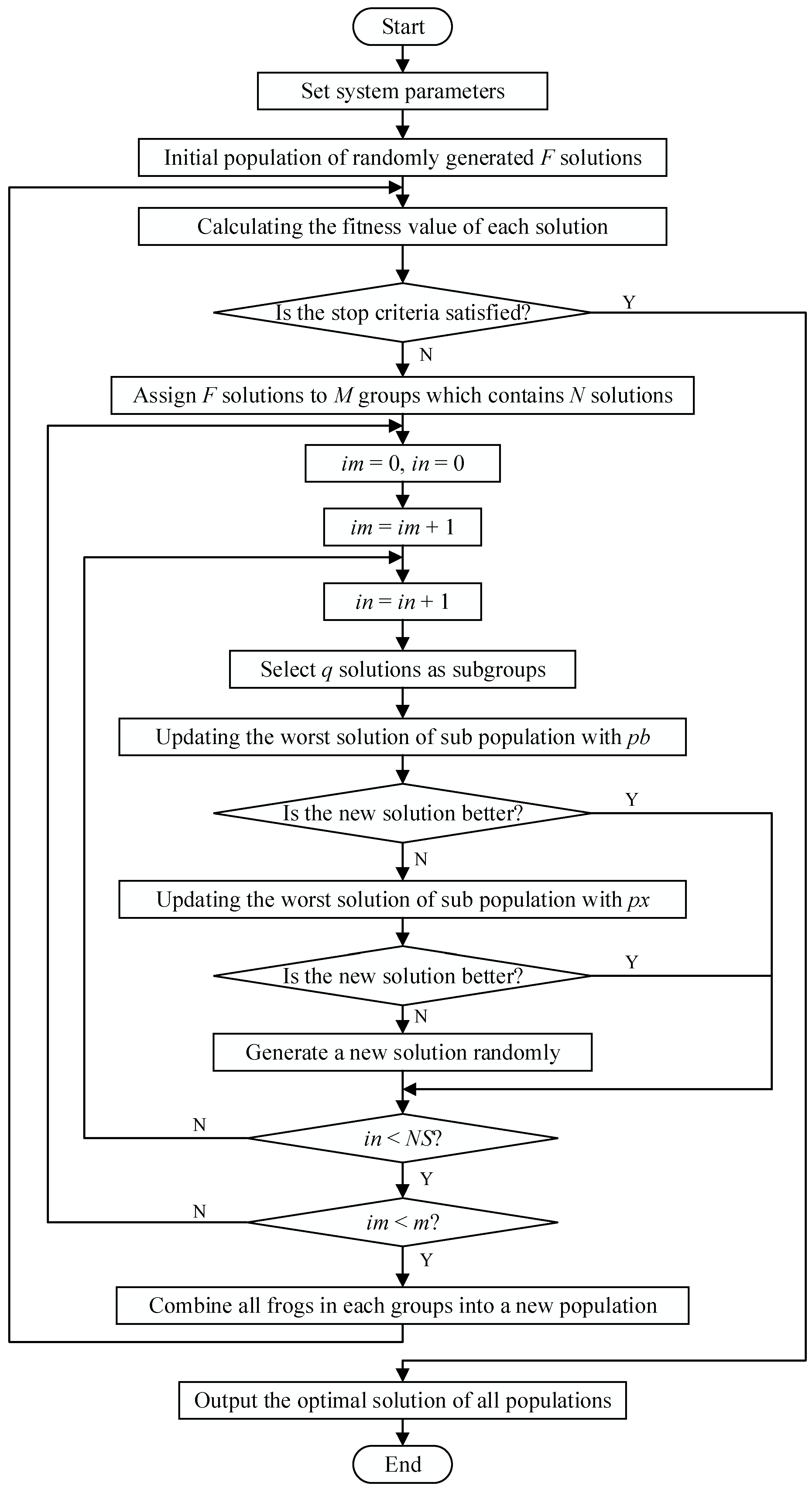
The standard SFLA is based on simulating the foraging behavior of frogs in nature. The specific flow is shown in Figure 2. After initializing the population, obtain F frogs, and calculate the fitness of each frog x. Sort all the frogs in descending order, and divide the population into m groups according to the sorting result so that each group contains n frogs; record the best frog px of the population, the best frog pb and the worst frog pw of each group, set im as the counter of the group and in as the counter of local evolution, and start the local evolution process; select q frogs in the im-th group to enter the sub-group and optimize the sub-group according to formula (16):
n e w   x   =   o l d   x   +   r a n d   ×   p b     p w
where rand is the random number following uniform distribution on [0,1].
If the position of the new frog is better than that of the old frog, then replace the old frog with the new frog; otherwise, replace the best frog pb from the group with the best frog px from the population, and continue to update according to Equation (16). If the frog is better, keep it; if not, randomly generate a new frog to replace the worst frog. Repeat the evolution process of the population until the number of local evolution NS is reached. Carry out the evolution of the next ethnic group until all ethnic groups have completed the evolution process.
After the evolution of all ethnic groups is completed, it is judged whether the frog with the best population has achieved the ideal result or has not changed many times. If the algorithm termination criterion is not met, all ethnic groups are mixed into a large population for the next population evolution process.
The overall flow of the SFLA is shown in Figure 2.

3.2. Solution Representation

This paper studies that the solution of FJSP-cSH needs to solve two key problems under the main goal of minimizing the makespan, that is, the optimal operation sequence of all jobs and the suitable machine allocation of all operations. Therefore, each solution to the problem is usually composed of two sequences, namely, job sequence and machine sequence. The job sequence represents the scheduling sequence of all operations, and the machine sequence represents the machine allocated to the corresponding operation.
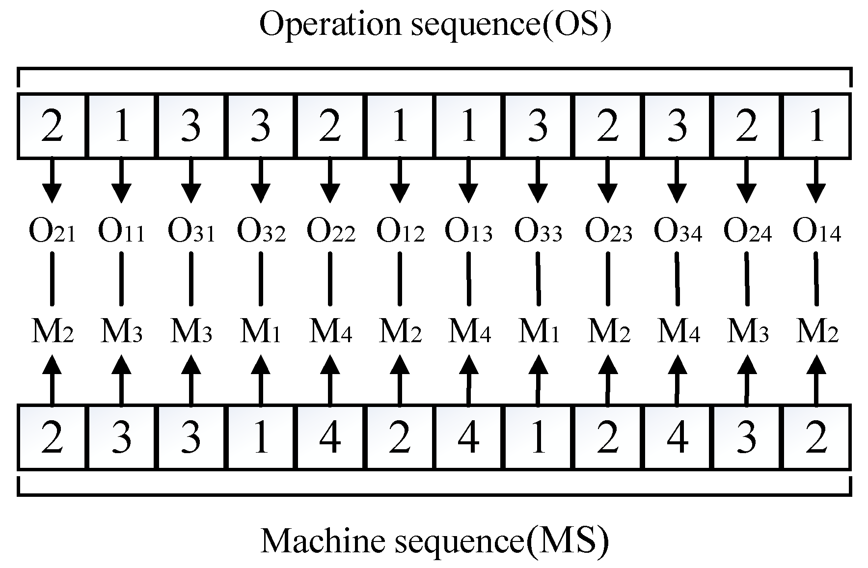
For example, there are four machines from three different work centers to process three jobs, all of which have only four operations and belong to different types. One of the solutions can be expressed in code as shown in Figure 3.
OS indicates the operation sequence of jobs, and MS indicates the sequence of machine selection. The number in the operation sequence is the serial number of the job. For example, the first occurrence of two in the first place indicates the first operation O21 of job 2, the second occurrence of two in the fifth place indicates the second operation O22 of job 2, and so on. The number in the machine selection sequence is the serial number of the machine, indicating the machine corresponding to the position operation. For example, the number two in the first place indicates that the machine in the operation O21 is the machine 2, and the number one in the fifth place indicates that the machine in the operation O22 is the machine 1.

3.3. Population Initialization

The following three rules are adopted to design the initial solution, aiming to enhance both the quality and diversity of the initial solution, thereby reducing algorithm iteration times and expediting its overall process. When generating the initial population, these three rules are used on average.

3.3.1. The Machine with the Earliest Idle Time for the Job That Arrives First

This rule means that the job that is finished in the previous operation earlier will have the priority to be processed in the next operation, and this job will be processed by the machine with the earliest idle time at present.
Firstly, for the first operation, randomly initialize the job sequence, and randomly arrange machines for processing corresponding jobs. After processing, the completion processing time of the first operation of all jobs and the completion processing time of all machines will be obtained, and two sequences of the completion processing time will be obtained by sorting in ascending order. Next, for the second operation, according to the two sequences of the completion processing time obtained in the first operation, select the job with the earliest completion processing time in the first operation. Among the optional machines in the second operation of this job, select the machine with the earliest completion processing time for processing. After the processing is completed, update the completion processing time of the machine. Then, select the job with the second earliest completion processing time in the first operation in turn, and select the machine for processing according to the same rules as above. After all jobs are processed, the completion processing time of the second operation for all jobs will be obtained, and the completion processing time sequence of the second operation will be obtained by sorting in ascending order. Afterwards, the remaining operations 3, 4,…, w are sorted according to the same rules as the operation 2.

3.3.2. The Machine with the Shortest Processing Time for the Job That Arrives First

This rule means that the job that is finished in the previous operation earlier will have the priority to be processed in the next operation, and the job will be processed by the machine with the shortest processing time.
Firstly, for the first operation, randomly initialize the job sequence. For the jobs in sequence, select the machine with the shortest processing time for the operations in turn. After the processing is completed, the completion processing time of the first operation of all jobs will be obtained, and the completion processing time sequence of the first operation will be obtained and sorted in ascending order. Next, for the second operation, according to the completion processing time sequence of the jobs obtained in the first operation, the jobs are selected in turn, and each job is processed by a machine with the shortest processing time. After the processing is completed, the completion processing time of the second operation of all jobs will be obtained, and the completion processing time sequence of the second operation will be obtained and sorted in ascending order. Afterwards, the remaining operations 3, 4,…, w are sorted according to the same rules as the operation 2.

3.3.3. Simple Randomly Generated Solution

This rule refers to the method of randomly generating an operation sequence and randomly selecting the corresponding machines to generate a machine sequence. The random generation method is to enhance the diversity of the population and avoid the obvious local characteristics of the initial population, which would cause the algorithm to be trapped into the local optimum.

3.4. Population Division

Population division is an indispensable step in the SFLA, and a prerequisite for the later process of seeking local evolution. The F frogs in the population are divided into m groups, and each group contains n frogs. The division rules are as follows: Sort the F frogs in the population according to their fitness. Divide the first frog into group 1, the second frog into group 2, the m-th frog into group m, the m + 1 frog back into group 1, the m + 2 frog back into group 2, and so on, until all frogs are divided.

3.5. Local Evolutionary Process

In the SFLA, the evolutionary optimization process of each sub-population is independent of each other. The essence is to improve the inferior solution according to the superior solution. For FJSP-cSH, each solution that is expressed by an operation sequence and a machine sequence is discrete. Therefore, the step size formula and position update formula using the standard SFLA are not applicable.
The new local evolutionary strategy used in this paper is proposed and described below.
new pw = δ (pwpb)
new pw = δ (pwpx)
The jump size δ and rules ⨁ of local evolutionary strategy are described below.

3.5.1. The Jump Size of the FJSP-cSH Based on Gravity Search Algorithm

In the SFLA, rand is a random value in the given [0,1] interval, and the probability transformation can be selected according to the evolution speed of the solution, and the transformation step size is limited by the maximum step size and the minimum step size. This fixed parameter selection method limits the evolution freedom of the solution.
In the FJSP-cSH, the updating strategy of the gravity search algorithm is used to determine the evolution parameters δ. The specific rules are as follows:
There is a mutual attraction between the solution of population and the solution of sub-population, which is determined by the quality of the solution and the distance between the two solutions, and the quality of the solution can be expressed by fitness. In the solution space, each solution gets its acceleration from the attraction of other solutions, and the solution with a greater mass (higher fitness) provides greater acceleration, thus making the poor solution move towards the optimal solution. The gravitational formula used to determine the value of δ is shown in Equation (19).
δ   =   G   t a r g e t p w   ×   t a r g e t p b h a m m i n g p w , p b
where G represents the gravitational constant, which is used to control the value of δ between [0,1]; and target represents the objective function value of frogs, which is calculated according to the objective linear weighting; and hamming represents the difference between two frogs in coding methods, which is calculated by the hamming distance between two decoding codes.
The introduction of gravitational search rules makes up for the weakness of the standard SFLA’s local search ability and its tendency to fall into the local optimum. In the initial SFLA, the evolution speed of the poor frog will be given directly according to the system requirements. If the evolution speed is too fast, the local search will be lost. After embedding GSA, the gravity is determined by the mass and distance between the poor frog and the better frog, which further affects the evolution speed. In the case of a long distance, the jumping distance of the worst frog is short, which will not cause a local deletion. Of course, the control of gravity constant G can still affect the evolution speed of the algorithm. In order to make the update step reasonably distributed in the range of [0,1], the value of G is determined by two solutions of the maximum gap of the population in each iteration.

3.5.2. The Jump Rules of the FJSP-cSH

The specific evolutionary steps of the worst solution are introduced below.
First, the worst solution pw is updated according to the local optimal solution pb (Equation (17)). Because the job is processed by moving in parallel sequential movement mode, the intersection only occurs in the same operation. Take the processing of all jobs in a certain operation as an example, and the updating steps are as follows:
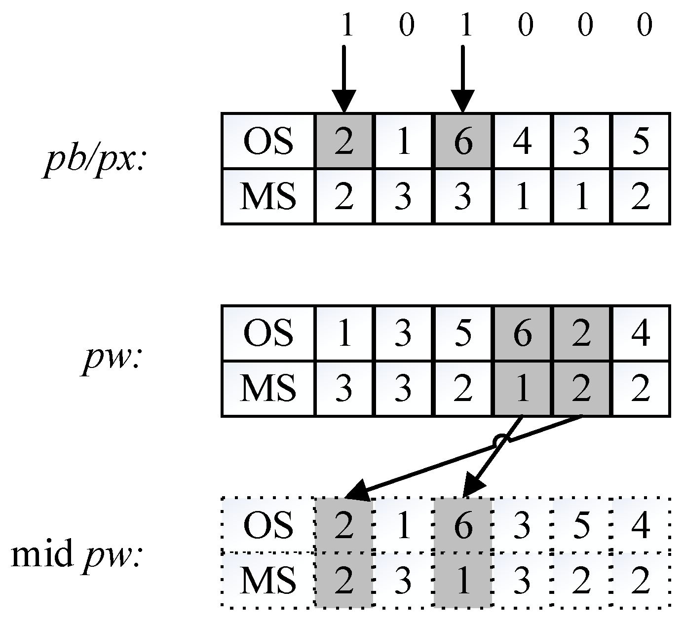
Update of operation sequence: First, a random 0~1 sequence is generated. Then, the operation corresponding to position 1 in the random number sequence will use the operation of the pb/px solution. After arranging all positions 1, the remaining positions 0 are filled in according to the sequence of unfinished operations in pw solution. The machine number moves with the operation number. As shown in Figure 4, in the operation sequence of a certain operation of six jobs, the random number 1 appears at position 1 and position 3. According to the optimal solution pb/px, the operation 2 remains in position 1, and the operation 6 remains in position 3. According to the worst solution pw, the remaining operation sequences are 1, 3, 5, and 4, which are sequentially filled in position 2, position 4, position 5, and position 6. The machine corresponding to the operation is consistent with the worst solution pw.
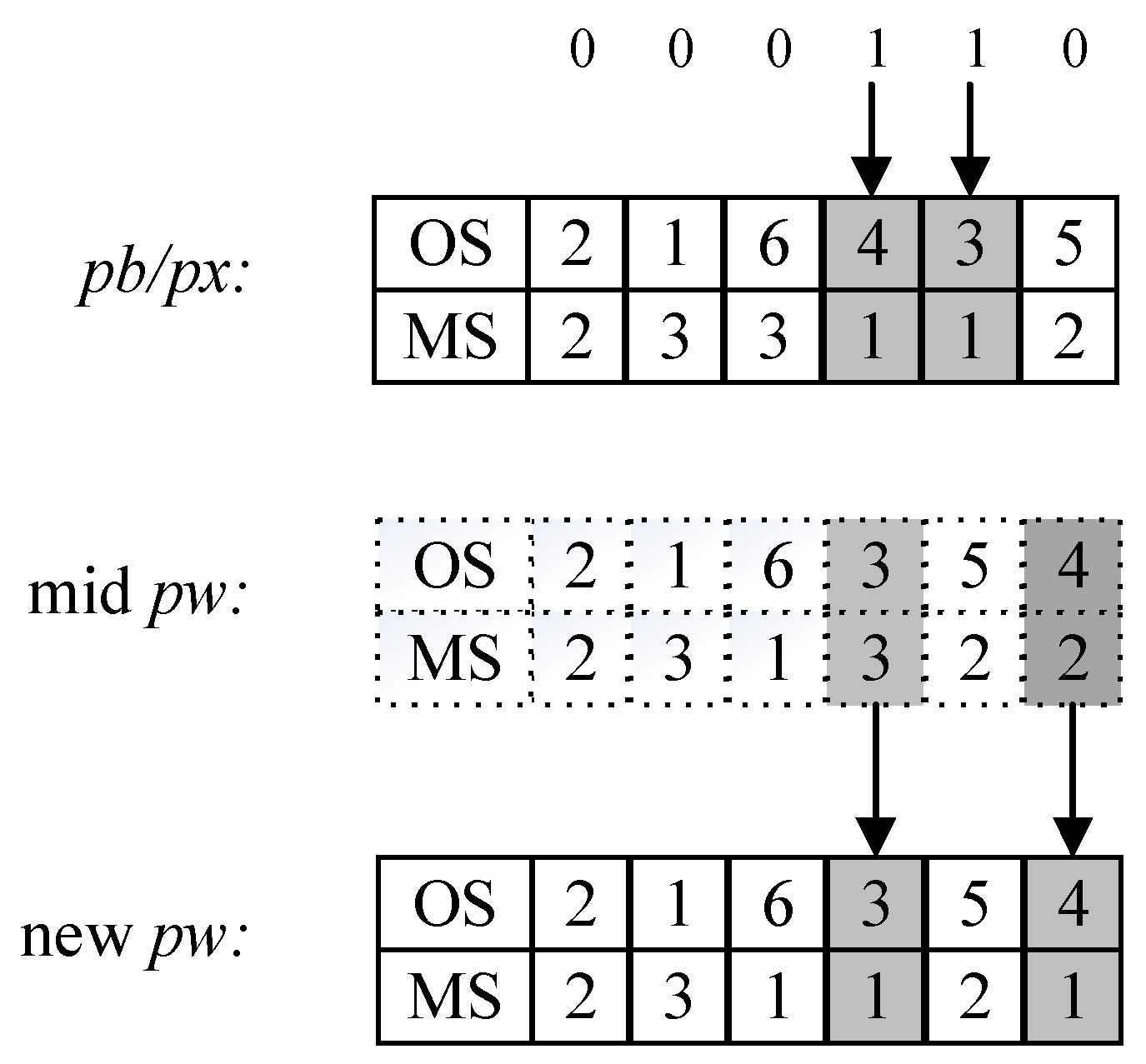
Update the machine sequence: First, generate a random 0~1 sequence. Then, update all the machines corresponding to the operation where the random number 1 appears, so that the machine number of this operation is the machine number of the pb/px solution. The machine number in other locations is unchanged, and the operation number is unchanged. As shown in Figure 5, the random number 1 appears at position 4 and position 5. According to the optimal solution pb/px, the process 4 is kept in the machine 1, and the process 3 is kept in the machine 1, and the machines of other operations remain unchanged. Finally, a new solution can be obtained.
Similar to the standard SFLA process, it is necessary to compare the fitness of the new solution with that of the old solution after the update process is completed. If the fitness of the new solution pw generated after crossover is not as good as the original pw, the global optimal solution px is used to update the worst solution pw (Equation (18)).
If the update effect is still unsatisfactory, a new solution needs to be generated to replace the worst solution. Compared with the operation through which the standard SFLA randomly generates new solutions, the uncertainty of evolution direction increases, which has a great influence on the speed of algorithm optimization. In this paper, the SFLA-uGSA uses the method of individual mutation to generate new solutions. Mutation is used in order to maintain the diversity of the population and to overcome premature convergence. The mutation operations are as follows: (1) Randomly exchange the order of jobs in the same process. (2) Randomly select a certain operation to change its machine. (3) Randomly select the sequence of jobs in a certain operation and change it to the same sequence as that of the previous operation. Each operation is randomly selected from three mutation methods, with an equal probability assigned to each method. If the fitness of the new solution by the mutated operation is better than that of the original worst solution, the original worst solution will be replaced by the new solution, otherwise, a new solution will be randomly generated to replace the original worst solution.

3.6. Population Shuffling

After all the groups have completed the evolutionary optimization process, the shuffling operator is performed to combine all the groups into a new large population, and the whole population is reordered according to fitness. Meanwhile, the best frog px of the new population is obtained and updated. The termination criterion of the algorithm is checked, that is, whether the specified number of population cycles m is completed. If it is met, the algorithm is terminated. If not, the next population division and local evolution will be carried out until the termination criterion is met.

3.7. Algorithm Description

The detailed procedure of our improved SFLA-uGSA is described as follows (Algorithm 1):
Algorithm 1 Step description of improvd SFLA-uGSA
Step 1: Initialization phase.
  Step 1.1: Set the system parameters, such as the population size F, the number of groups m and the number of local evolution NS.
  Step 1.2: Read the file data, such as the number of jobs, the number of machines, the processing time, the handing time and the setup time.
Step 2: Generate the initial population according to three different rules that are established in Section 3.3, calculate the fitness of each frog, and determine the global optimal solution px.
Step 3: If the termination criterion is satisfied, output the global optimal solution px; otherwise, perform step 4.
Step 4: Divide the population F into m groups according to the rules of population division, and calculate the value of G of this generation of population.
Step 5: For each group i, i = 1, 2,…, m, perform local evolution process for NS times.
  Step 5.1: Determine the best solution pb and the worst solution pw in the group i.
  Step 5.2: Update the worst solution pw with the best solution pb according to the local updating evolution formula (Equation (17)), and a new solution is generated through gravitational calculation and renewal evolution. If the fitness of new solution is better than old solution pw, then let the new solution replace the old solution pw, perform step 5.5; otherwise, perform step 5.3.
  Step 5.3: Update the worst solution pw with the population best solution px according to the local updating evolution formula (Equation (18)), and a new solution is generated through gravitational calculation and renewal evolution. If the fitness of new solution is better than old solution pw, then let the new solution replace the old solution pw, perform step 5.5; otherwise, perform step 5.4.
  Step 5.4: Use individual mutation method to transform the worst solution pw, if the fitness of the new solution after transformation is better than that of the old solution before transformation, let the new solution replace the old solution pw, perform step 5.5; otherwise, randomly generate a new solution to replace the worst solution pw, perform step 5.5.
  Step 5.5: Update the group i.
Step 6: Shuffle the evolved groups, perform step 3.
It can be seen from the above procedure that the SFLA-uGSA not only performs several independent evolutionary processes within each group, but also enables the whole population to exchange information periodically through the population shuffling to ensure the global searching ability of the algorithm. The method generation of the initial population and the improvement of the local search method enhance the development ability of the optimization algorithm for the FJSP-cSH.

4. Multi-Objective Optimization: Model Rules and Algorithm Design

In this paper, when considering the FJSP-cSH with the makespan as the main objective, the two objectives of the total number of machine shutdowns and the total number of handing batches are optimized, and finally, the specific processing time (setup time and processing time are closely connected with each other) and the specific handling time are determined. In this section, the parallel sequential movement mode and the design of batch handling mode are mainly introduced, and the multi-objective solution method is described.

4.1. Parallel Sequential Movement Mode

In order to reduce the total number of machine shutdowns as much as possible, this paper adopts the method of continuous processing when the machine processes all jobs in the same operation, that is, parallel sequential movement mode. Parallel sequential movement mode not only considers the parallelism of processing, but also considers the continuity of processing. In order to meet this requirement, jobs should be handled according to the following rules: when the processing time of the previous operation is less than that of the next operation, the job which has been processed in the previous operation should be transferred to the next machine immediately, otherwise, the job which has been processed in the previous operation will be transferred to the next machine only when the number of jobs completed in the previous operation is enough to ensure the continuous processing of the next operation. In this way, the scattered time of the machine can be concentrated.
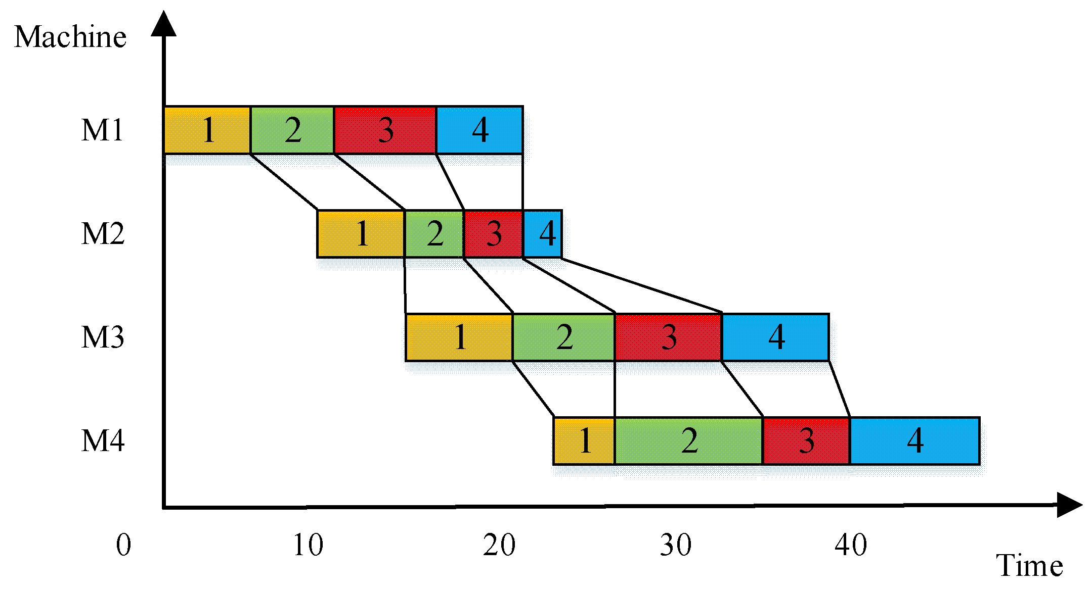
For example, only considering the processing time of jobs, when four different jobs are processed on four machines in succession, that is, when there are four operations, the parallel sequential movement mode can be shown in Figure 6.
As shown in Figure 6, when four jobs move to the machine 2 after being processed by the machine 1, because the processing time of the first operation is greater than that of the second operation, the jobs 1, 2, and 3 have to wait for a while before they can be processed. When four jobs move to the machine 3 after being processed by the machine 2, because the processing time of the second operation is less than that of the third operation, the third operation of job 1 can be processed directly after the second operation is finished, and the jobs 2, 3, and 4 are processed after the machine 3 is idle. When the four jobs move to the machine 4 after being processed by the machine 3, the time is relatively complicated. After executing the parallel movement mode, it will be found that there is a machine idle between the processing of job 1 and job 2. In order to ensure that the parallel sequential movement mode is adopted, the processing time of job 1 must be delayed to ensure the continuity of the processing time of job 2.

4.2. Batch Handling Mode Design

In order to reduce the batch handling tasks of jobs as much as possible, this paper designs a new handling mode of jobs for the solution with fixed processing time. In this paper, the parallel sequential movement mode is adopted to process jobs, so there is a certain slack time between the different operations of jobs, that is, during this time, the job can be handled freely. Without considering the limitation of the handling capacity of the handling equipment, the more jobs are handled in a single time, the less the total number of handling batches will be. Therefore, the handling of jobs between machines follows the following principles: (1) The handling time of jobs does not change the determined setup time and processing time. (2) In a single handling, the handling time is determined by the minimum value of the latest time in the transfer slack time interval of all jobs; that is, the completion handling time should not be greater than the start processing time of the next operation of all transferred jobs. (3) In a single handling, the number of jobs is determined by the number of all jobs to be handled that can meet the handling time.
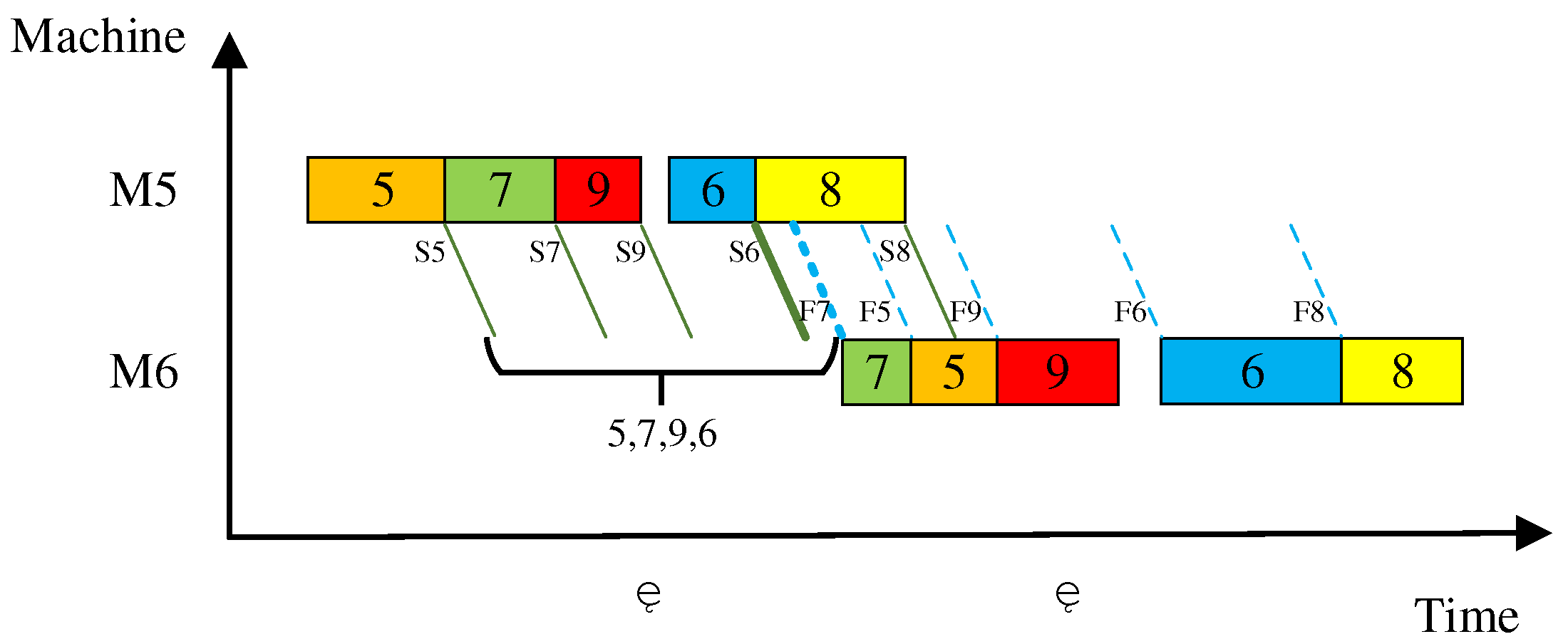
For example, there is a handling task of five jobs, and the handling direction is from machine 5 to machine 6. The handling time and the number of jobs to be handled can be shown in Figure 7.
As shown in Figure 7, the earliest handing time of all jobs (indicated by the solid line) and the latest handing time of all jobs (indicated by the dotted line) of the five jobs are calculated in sequence. The minimum latest handing time (indicated by F), that is, the latest completion handling time of the job 7, is selected as the end time of this handling without affecting the processing of the jobs in the next operation. Then, there are jobs 5, 7, 9, and 6 with the earliest handing time (indicated by S) before that. Therefore, the handling time is indicated by F7, and the number of jobs to be handled is four. Actually, the handing time can be arbitrarily set between S6 and F7 (indicated by the bold lines) without affecting the final result.

4.3. Pareto Ranking Method

The FJSP has been proved to be a NP-hard problem. The research of Pareto optimal method is considered as the result of this problem. In this paper, in order to achieve multi-objective optimization, the Pareto ranking method is used to sort the solutions of population and all groups, and one of the non-dominated solutions is set as the best solution.
When ranking the population, the group with the first-order non-dominated solution is selected first; that is, each goal of each solution of this group is no worse than that of other solutions. Then, the first-order group is removed from the population, and the group with the second-order non-dominated solution is found by the same method. Repeat this step until the population is completely divided into the various groups. The groups are ranked according to Pareto level, while individuals within groups are ranked according to the priority of goals. The rule of individual sequencing within a group is that the makespan is the main goal, the total number of machine shutdowns is the second, and finally, the total number of handling batches is considered.

5. Experimental Results

In this section, the MATLAB R2020b software is used for the calculation experiment to evaluate the performance of the SFLA-uGSA. Firstly, a Design of Experiment (DOE) is carried out to determine the optimal parameter combination. Secondly, the algorithm is tested by a single objective with standard examples. The results are compared with those of other articles, and the effectiveness of this algorithm is obtained. Thirdly, compared with single-objective optimization, the superiority of the algorithm in multi-objective optimization is analyzed. Finally, an example with the setup time and the handling time is designed to analyze the experimental results. The implementation has been performed on a computer with a 2.40 GHz Core (TM) i5 CPU with 16 GB RAM memory.

5.1. Algorithm Parameter Setting

Before applying the SFLA-uGSA to all the instances, a DOE based on MK07 from the article by Brandimarte [24] has been conducted for parameter tuning, and the makespan is calculated as the evaluation criterion. The desirable parameter combinations are as follows: MS = {50, 100, 150, 200}, NS = {5, 10, 15, 20}, F = {30, 60, 90, 120}, and m = {3, 6, 10, 15}. The running time of the experiment is limited to 100 s to prevent the excessive sacrifice of time for the accuracy of the results. Figure 8 shows the average effect results under different parameters.
The results show that in the application of small-sized and medium-sized examples, the algorithm parameters in this paper are set as follows to achieve better performance: the times of global search MS = 100; the times of local evolution NS = 10; the number of population F = 90; the number of group m = 6; the number of individuals in each group n = 15.

5.2. Algorithm Effectiveness Analysis

When analyzing the effectiveness of the algorithm, according to the standard examples, only the makespan is calculated and compared with the optimization algorithms in other articles. We select eight benchmark problems from the article by Brandimarte [24] and the article Kacem [25] to be tested. The SFLA-uGSA is an algorithm proposed in this paper, which runs 10 times to record the optimal value and the average deviation. Five evolutionary algorithms, CCGA [26], GRASP [27], SLGA [28], PSO [29], and MSCGA [30], are selected for comparison. Table 2 shows the results of this experiment, where α represents the number of jobs, β represents the number of machines, Size represents the number of operations, LB represents the known optimal solution, and SD represents the average deviation.
The experimental results show that the algorithm runs well in the problem MK03, Kacem01, Kacem02, Kacem03, and Kacem04, which is the best at present, and runs generally in the problems MK06, MK07, and Kacem05, which are better than some algorithms but not the best. This is because the algorithm follows the parallel sequential movement mode when decoding the solution. One machine needs to work continuously when processing the same operation. Some jobs that can be processed in advance are delayed to ensure the continuous operation of the machine. It can be predicted that the greater the number of work procedures, the greater the deviation of the completion time from the standard time, which is the inevitable result of getting lower shutdown. Overall, the algorithm can stably get a satisfactory solution by minimizing the makespan in small-scale problems.
In the parallel sequential movement mode, in order to further explore the superiority of the strategies introduced in this paper, such as population initialization rules and local evolutionary rules, the proposed SFLA-uGSA is compared with the standard SFLA. A total of 20 benchmark problems (rdata, where most operations can be assigned to a few different machines.) from the article Hurink [31] are selected to be tested, and every example runs 10 times. Table 3 shows the results of this experiment, where Best represents the optimal value and the Average represents the average value.
The data in Table 3 shows that the SFLA-uGSA has better results and stability than the SFLA. Compared with the known optimal solution LB, both the SFLA-uGSA and the SFLA achieve the best in a few small-scale examples, but it is difficult to achieve the LB in other examples, which is the inevitable result of following the parallel sequence movement mode. In the comparison between the SFLA-uGSA and the SFLA, the overall performance of the former is superior to that of the latter in terms of optimal value, average value, and stability.
The influence of Pareto ranking method on the multi-objective solution is analyzed by comparing it with the single-objective solution. Taking the MK03 problem as an example, ten experiments were run to extract one solution from the multi-objective Pareto optimal solution group each time. The results were compared with the previous single-objective solution. The results are shown in Table 4. Target 1 represents the makespan. Target 2 represents the total number of machine shutdowns. Target 3 represents the total number of handling batches.
The experimental results show that in the single-objective optimization, the makespan reaches the minimum, but the total number of machine shutdowns and the total number of handling batches are relatively large, which can result in machine abrasion and energy consumption. In the multi-objective optimization, the solution is more in line with the multi-objective co-optimization situation by reducing the number of machine shutdowns and handling batches with a small amount of sacrifice to the goal of the makespan.

5.3. Example Analysis

In this paper, a small practical example is designed to prove the effectiveness of the model in achieving multi-objective optimization under the constraints of machine setup and job handling. The details of the design are as follows: the processing time is adapted from the problem MK02 in the article by Brandimarte [24]. The setup time refers to the ratio of setup time to processing time in the article by Kong et al. [32] and the article by Zeng et al. [33]. The handling time refers to the ratio of handling time to processing time in the article by Tian et al. [34]. Table 5 shows the distribution of jobs in different types. Table 6 shows the distribution of machines in different work centers. Table 7 shows the job processing time. Table 8 shows the machine setup time. Table 9 shows the handling time between the work centers.
Through the experimental operation of this example, the results are as follows: the makespan is 36, the total number of machine shutdowns is 7, and the total number of handling batches is 17.
The specific scheduling information is shown in Table 10, Table 11 and Table 12 below. Table 10 shows the scheduling information of jobs, that is, the processing situation of every operation of each job, including the setup time and the processing time. Table 11 shows the scheduling information of machines, that is, the working and shutdown of each machine. At time 0, we default that the machine is not working, so it needs to be counted as one shutdown. At this time, for the machine that enters the processing state immediately, the time of shutdown is 0. Table 12 shows the scheduling information of handling batches, that is, the job number, start–end position, and start–end time of each handling batch. In addition, the earliest handling time and the latest handling time are given under the condition of slack time.
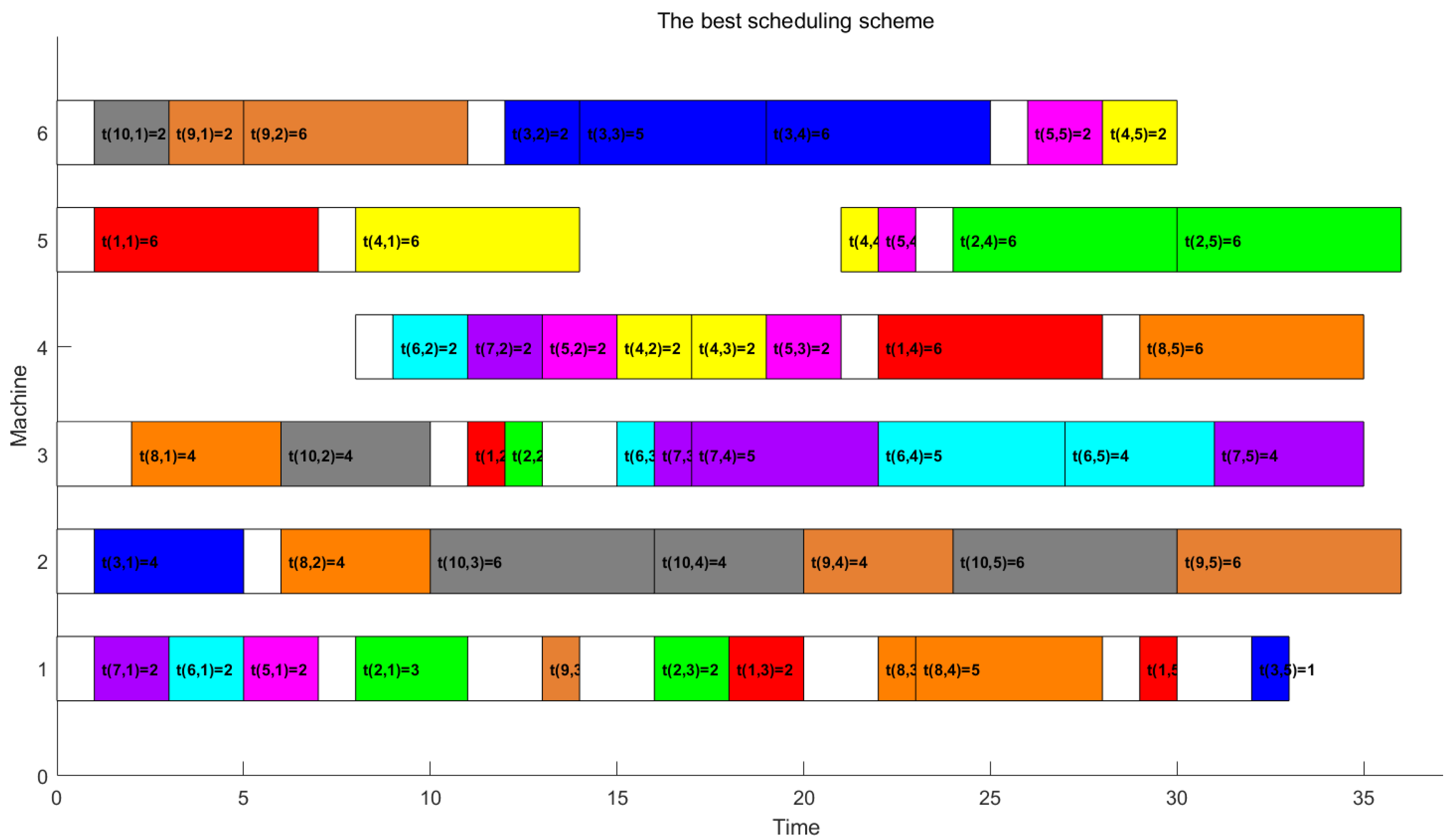
Figure 9 shows the Gantt chart of the scheduling situation. The white rectangle is the process of machine setup, and the colored rectangle is the process of job processing. The left and right sides of the rectangle correspond to the start time and the completion time of machine work. The length of the rectangle corresponds to the time span of the machine work. Different colored rectangles represent different jobs. The text in the rectangular box shows the job number, operation number, and processing time. For example, t(8,1) = 4 indicates that the processing time of the operation 1 of job 8 is 4, and the white rectangle in front of the orange rectangle indicates the setup time of the machine 3.
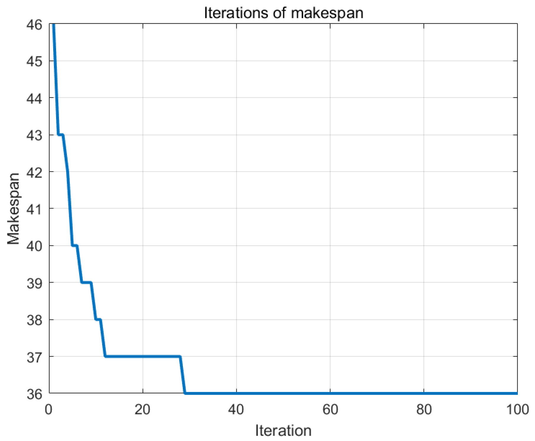
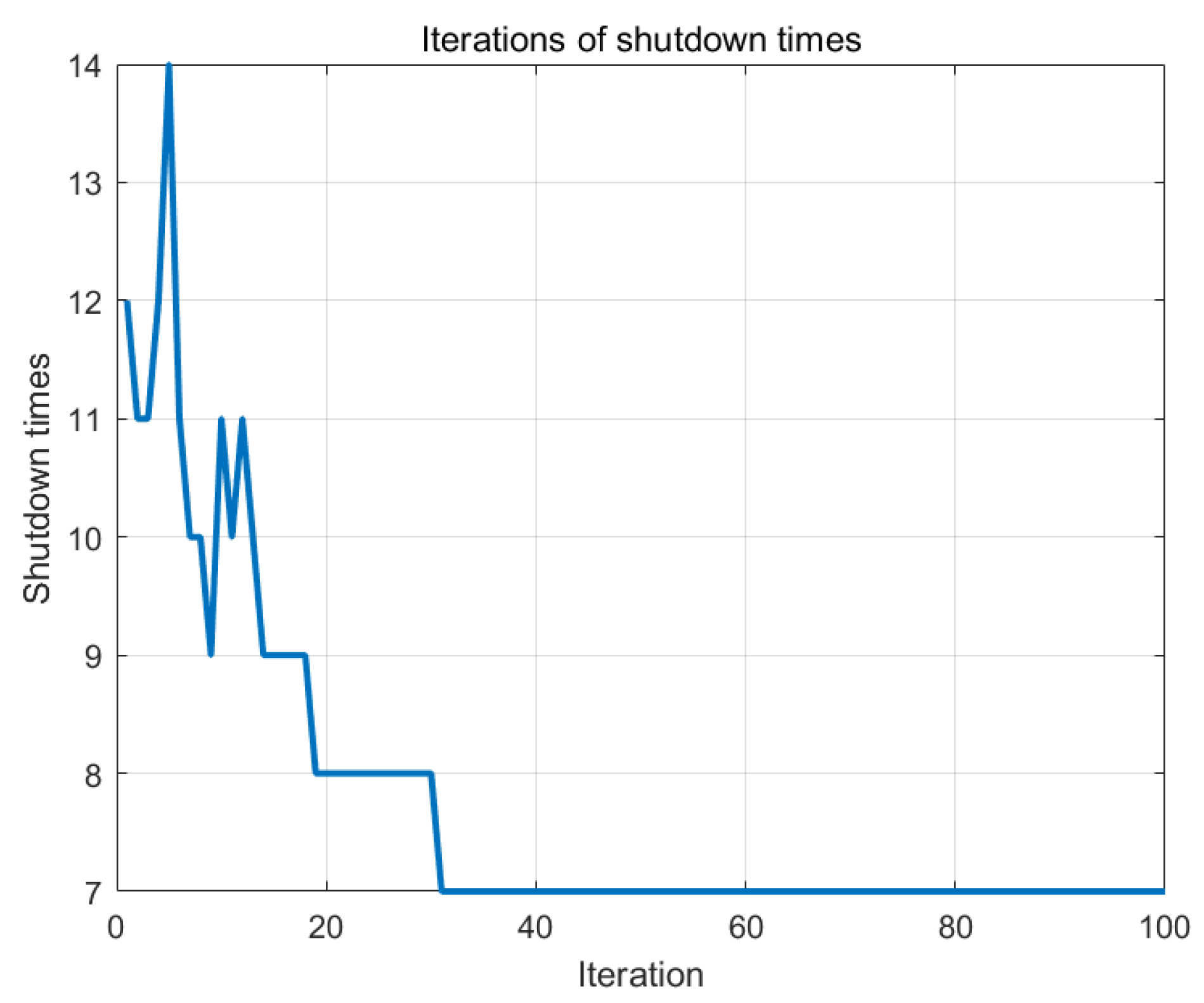
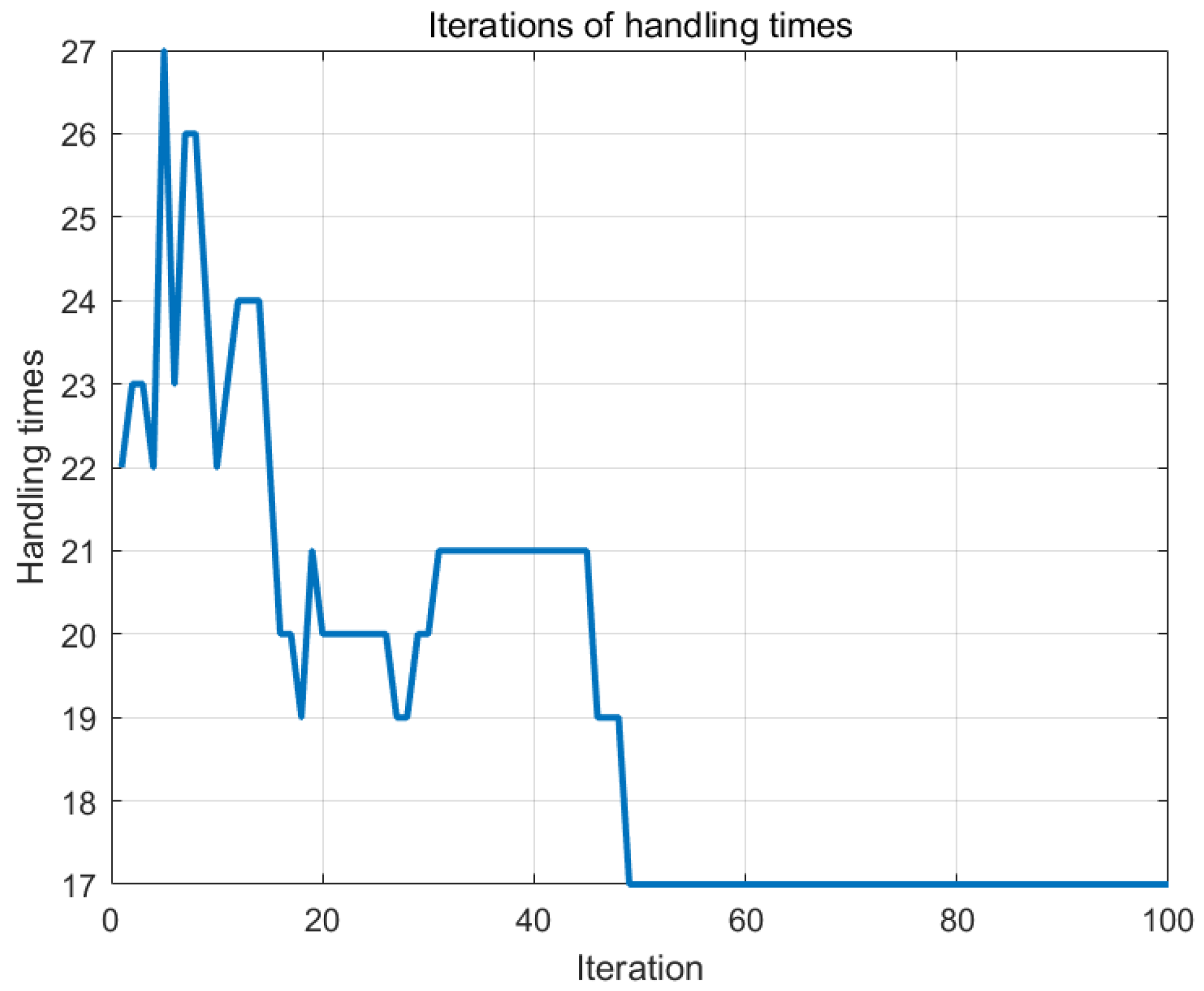
Figure 10, Figure 11 and Figure 12 are, respectively, the iterative results of the makespan, the number of machine shutdowns, and the number of handling batches of the optimal solution after ranking the multi-objectives. It can be seen that in the initial stage of the algorithm operation, the makespan will be optimized quickly as a higher priority goal, and the number of machine shutdowns and handling batches will be gradually reduced in the jump. The number of machine shutdowns and the number of handling batches will change during the search for the minimum makespan, which will still decrease in the subsequent search process, thus realizing the overall optimization of the scheme.
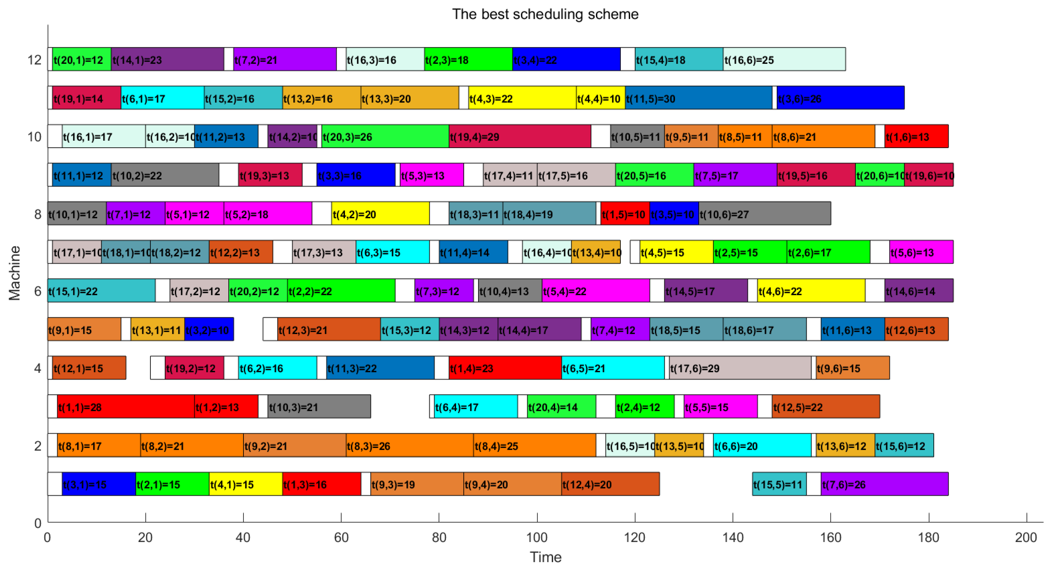
In order to prove that the algorithm designed in this paper is still effective in solving large-scale application examples, a new adaptation example is designed for experiments. This example includes five types of jobs, 20 jobs, six processes, five work centers, and 12 machines. The processing time is adapted from the problem Sm01.1 from the article [7]. The design strategy of setup time and handling time refers to the same small-scale example as above. The processing time of the example is evenly distributed within the interval [10,30]. The setup time of the example is evenly distributed within the interval [0,4]. The handling time of the example is evenly distributed within the interval [1,7].
Figure 13 shows the scheduling Gantt chart of the optimal solution, and the information form is explained in the same way as Figure 9. The objectives of the optimal solution are as follows: the makespan is 185, the total number of machine shutdowns is 17, and the total number of handling batches is 54.

6. Conclusions

This paper proposes a multi-objective FJSP-cSH model, and designs an improved SFLA-uGSA algorithm to solve it. The feasibility of the model and the effectiveness of the algorithm are proved in the final example test. The purpose of this paper is not only to quickly implement the solution, but also to increase the constraints and target coordination of the problem model considering the actual needs of modern factories. In the aspect of model construction, the following two manufacturing factory conditions are considered. On the one hand, the jobs have the characteristics of multi-variety and small-batch. The machines are distributed to different work centers according to their functions and positions. On the other hand, considering the current situation of machine setup and job handling in actual factory production scheduling, it increases the setup time of machines when processing different types of jobs and the handling time when jobs are handled between different work centers. In the aspect of algorithm design, the improved SFLA which is combined with the GSA to update the position is proposed. The scheduling plan is arranged according to the parallel sequential movement mode, and finally the Pareto ranking method is introduced to solve the multi-objective collaborative optimization problem. In the final experimental comparison and analysis, it can be seen that the algorithm is very effective in solving the multi-objective problem under these special constraints. In the final experiment comparison and analysis, the superiority of the SFLA-uGSA in solving multi-objective FJSP is proved by the comparison of standard examples. And, the effectiveness of the SFLA-uGSA in solving multi-objective FJSP-cSH is proved by the designed example.
The future work is mainly carried out from the following two aspects: First, try to break through the limitation of the same number of job operations in parallel sequential movement mode, so that the algorithm can be applied to a wider range of situations. Second, combine with other efficient optimization algorithms to further improve the superiority of the algorithm and the ability to obtain Pareto optimal solution. In addition, in the actual intelligent manufacturing factory, the dynamic performance of the scheduling plan and the stochastic performance of the machine are both uncertain factors. The consideration of these factors will make the scheduling model closer to the real manufacturing world, which is more complicated but interesting and necessary.

Author Contributions

Conceptualization, J.K. and Y.Y.; methodology, Y.Y. and J.K.; software, J.K.; validation, Y.Y. and J.K.; formal analysis, Y.Y. and J.K.; investigation, Y.Y. and J.K.; resources, J.K.; data curation, Y.Y.; writing—original draft preparation, Y.Y. and J.K.; writing—review and editing, Y.Y. and J.K.; visualization, Y.Y.; supervision, J.K.; project administration, J.K. and Y.Y.; funding acquisition, J.K. All authors have read and agreed to the published version of the manuscript.

Funding

This research was funded by the Humanities and Social Science Youth foundation of the Ministry of Education of China, grant number 20YJC630054.

Institutional Review Board Statement

Not applicable.

Informed Consent Statement

Not applicable.

Data Availability Statement

The data presented in this study are available upon request from the corresponding author. The data are not publicly available due to privacy.

Conflicts of Interest

The authors declare no conflicts of interest.

Abbreviations

Description of the symbols.
SymbolsDefinitions
Jithe set of jobs (i = 1, 2,…, n)
Oijthe set of operations (i = 1, 2,…, n; j = 1, 2,…, w; Oij represents the j-th operation of job i)
Mkthe set of machines (k = 1, 2,…, m)
MUijthe set of work centers, that is, the optional machines’ set of the operation Oij
TPijkthe processing time of operation Oij on machine Mk
TSijkthe setup time of operation Oij on machine Mk
TCk1k2handling time from machine Mk1 to machine Mk2
La sufficiently large positive number (or constraint)
Cithe completion time of job Ji
Cmaxthe makespan of order task
T P i j k B the start processing time of operation Oij on machine Mk
T P i j k E the completion processing time of operation Oij on machine Mk
T S i j k B the start setup time of operation Oij on machine Mk
T S i j k E the completion setup time of operation Oij on machine Mk
T C i j B start handling time after operation Oij
T C i j E completion handling time after operation Oij
NOHthe number of handling tasks
Ththe set of handling tasks (h = 1, 2,…, NOH)
T h B the start handling time of the handling task h
T h E the completion handling time of the handling task h

References

  1. Chaudhry, A.I.; Khan, A.A. A research survey: Review of flexible job shop scheduling techniques. Int. Trans. Oper. Res. A J. Int. Fed. Oper. Res. Soc. 2016, 23, 551–591. [Google Scholar] [CrossRef]
  2. Andy, H. Transfer-robot task scheduling in job shop. Int. J. Prod. Res. 2021, 59, 813–823. [Google Scholar]
  3. Yige, S.; Sai-Ho, C.; Xin, W.; Hoi-Lam, M. Novel robotic job-shop scheduling models with deadlock and robot movement considerations. Transp. Res. Part E 2021, 149, 102273. [Google Scholar]
  4. Soroush, F.; Reza, T.; Mehdi, F.; Behdin, V. Scheduling of Multi-Robot Job Shop Systems in Dynamic Environments: Mixed-Integer Linear Programming and Constraint Programming Approaches. Omega 2023, 115, 102770. [Google Scholar]
  5. Allahverdi, A.; Ng, C.; Cheng, T.; Kovalyov, M. A survey of scheduling problems with setup times or costs. Eur. J. Oper. Res. 2006, 187, 985–1032. [Google Scholar] [CrossRef]
  6. Zhang, C.; Zhou, Y.; Peng, K.; Li, X.; Lian, K.; Zhang, S. Dynamic flexible job shop scheduling method based on improved gene expression programming. Meas. Control 2020, 54, 002029402094635. [Google Scholar] [CrossRef]
  7. Behnke, D.; Geiger, M.J. Test Instances for the Flexible Job Shop Scheduling Problem with Work Centers. Logist.-Manag. 2012. [Google Scholar] [CrossRef]
  8. Govi, D.; Rizzuto, A.; Schipani, F.; Lazzeri, A. A Two-stage Genetic Algorithm for a Novel FJSP with Working Centers in a Real-world Industrial Application. In Proceedings of the 2nd International Conference on Innovative Intelligent Industrial Production and Logistics, Online, 25–27 October 2021; pp. 75–83. [Google Scholar]
  9. Pal, M.; Mittal, M.L.; Soni, G.; Chouhan, S.S.; Kumar, M. A multi-agent system for FJSP with setup and transportation times. Expert Syst. Appl. 2023, 216, 119474. [Google Scholar] [CrossRef]
  10. Feng, Y.J.; Kong, J.L. Multi-Objective Hybrid Flow Shop Scheduling in Parallel Sequential Mode While Considering Handling Time and Setup Time. Appl. Sci. 2023, 13, 3563. [Google Scholar] [CrossRef]
  11. Wu, Q.; Ji, Z.; Wu, D. Cooperative hybrid particle swarm optimization algorithm for job-shop scheduling problems. Comput. Eng. Appl. 2016, 52, 266–270. [Google Scholar]
  12. Vital-Soto, A.; Azab, A.; Baki, F.M. Mathematical modeling and a hybridized bacterial foraging optimization algorithm for the flexible job-shop scheduling problem with sequencing flexibility. J. Manuf. Syst. 2020, 54, 74–93. [Google Scholar] [CrossRef]
  13. Liu, Z.; Wang, J.; Zhang, C.; Chu, H.; Ding, G.; Zhang, L. A hybrid genetic-particle swarm algorithm based on multilevel neighbourhood structure for flexible job shop scheduling problem. Comput. Oper. Res. 2021, 135, 105431. [Google Scholar] [CrossRef]
  14. Alzaqebah, M.; Jawarneh, S.; Alwohaibi, M.; Alsmadi, M.K.; Almarashdeh, I.; Mohammad, R. Hybrid Brain Storm Optimization algorithm and Late Acceptance Hill Climbing to solve the Flexible Job-Shop Scheduling Problem. J. King Saud Univ.-Comput. Inf. Sci. 2020, 34, 2926–2937. [Google Scholar] [CrossRef]
  15. Liu, X. Improved Multi-Objective Composed Optimization Algorithm Studying for Flexible Job-Shop Scheduling Problems. Master’s Thesis, Jilin University, Changchun, China, 2020. [Google Scholar]
  16. Yan, S.; Zhang, G.; Sun, J.; Zhang, W. An improved ant colony optimization for solving the flexible job shop scheduling problem with multiple time constraints. Math. Biosci. Eng. MBE 2023, 20, 7519–7547. [Google Scholar] [CrossRef]
  17. Teekeng, W.; Thammano, A. A Combination of Shuffled Frog Leaping and Fuzzy Logic for Flexible Job-Shop Scheduling Problems. Procedia Comput. Sci. 2011, 6, 69–75. [Google Scholar] [CrossRef]
  18. Ramya, G.; Chandrasekaran, D.M. Shuffled frog leaping algorithm approach to employee timetabling and job shop scheduling. Int. J. Internet Manuf. Serv. 2014, 3, 178–203. [Google Scholar] [CrossRef]
  19. Wang, Z.; Zhang, D.; Wang, B.; Chen, W. Research on Improved Strategy of Shuffled Frog Leaping Algorithm. In Proceedings of the 2019 34th Youth Academic Annual Conference of Chinese Association of Automation (YAC), Jinzhou, China, 6–8 June 2019. [Google Scholar]
  20. Lei, D.; Guo, X. A shuffled frog-leaping algorithm for job shop scheduling with outsourcing options. Int. J. Prod. Res. 2015, 54, 4793–4804. [Google Scholar] [CrossRef]
  21. Meng, L.; Ren, Y.; Zhang, B.; Li, J.Q.; Sang, H.; Zhang, C. MILP Modeling and Optimization of Energy-Efficient Distributed Flexible Job Shop Scheduling Problem. IEEE Access 2020, 8, 191191–191203. [Google Scholar] [CrossRef]
  22. Karakoyun, M.; Ozkis, A.; Kodaz, H. A new algorithm based on gray wolf optimizer and shuffled frog leaping algorithm to solve the multi-objective optimization problems. Appl. Soft Comput. J. 2020, 96, 106560. [Google Scholar] [CrossRef]
  23. Ramya, G.; Chandrasekaran, M.; Arulmozhi, P. Optimization of production cost for integrating job shop scheduling with production resources. Mater. Today Proc. 2020, 37, 1839–1844. [Google Scholar] [CrossRef]
  24. Brandimarte, P. Routing and scheduling in a flexible job shop by tabu search. Ann. Oper. Res. 1993, 41, 157–183. [Google Scholar] [CrossRef]
  25. Kacem, I.; Hammadi, S.; Borne, P. Approach by localization and multi-objective evolutionary optimization for flexible job-shop scheduling problems. IEEE Trans. Syst. Man Cybern. Part C 2002, 32, 1–13. [Google Scholar] [CrossRef]
  26. Rou, L.Y.; Asmuni, H. A study of cooperative co-evolutionary genetic algorithm for solving flexible job shop scheduling problem. Int. J. Comput. Inf. Eng. 2010, 4, 1849–1854. [Google Scholar]
  27. Kemmoé-Tchomté, S.; Lamy, D.; Tchernev, N. An effective multi-start multi-level evolutionary local search for the flexible job-shop problem. Eng. Appl. Artif. Intell. 2017, 62, 80–95. [Google Scholar] [CrossRef]
  28. Chen, R.; Yang, B.; Li, S.; Wang, S. A self-learning genetic algorithm based on reinforcement learning for flexible job-shop scheduling problem. Comput. Ind. Eng. 2020, 149, 106778. [Google Scholar] [CrossRef]
  29. Ding, H.; Gu, X. Improved particle swarm optimization algorithm based novel encoding and decoding schemes for flexible job shop scheduling problem. Comput. Oper. Res. 2020, 121, 104951. [Google Scholar] [CrossRef]
  30. Wang, C.; Li, Y.; Li, X. Solving flexible job shop scheduling problem by a multi-swarm collaborative genetic algorithm. J. Syst. Eng. Electron. 2021, 32, 261–271. [Google Scholar]
  31. Hurink, J.; Jurisch, B.; Thole, M. Tabu search for the job-shop scheduling problem with multi-purpose machines. Oper. Res. Spektrum 1994, 15, 205–215. [Google Scholar] [CrossRef]
  32. Kong, J.; Yuan, C.; Yang, F.; Jia, G. Multi-objective flow shop batch scheduling with separable processing time and setup time under parallel-sequence-transfer mode. Syst. Eng.-Theory Pract. 2017, 37, 2882–2896. [Google Scholar]
  33. Zeng, Q.; Chang, M.; Wang, M.; Zhang, J. Multi-objective optimization method for FJSP under mixed work calendars. J. Chongqing Univ. 2019, 42, 10–26. [Google Scholar]
  34. Tian, M.; Zhang, G.; Liu, R. Solve FJSP Considering Transport Time via Particle Swarm Genetic Hybrid Algorithm. Oper. Res. Manag. Sci. 2019, 28, 78–88. [Google Scholar]
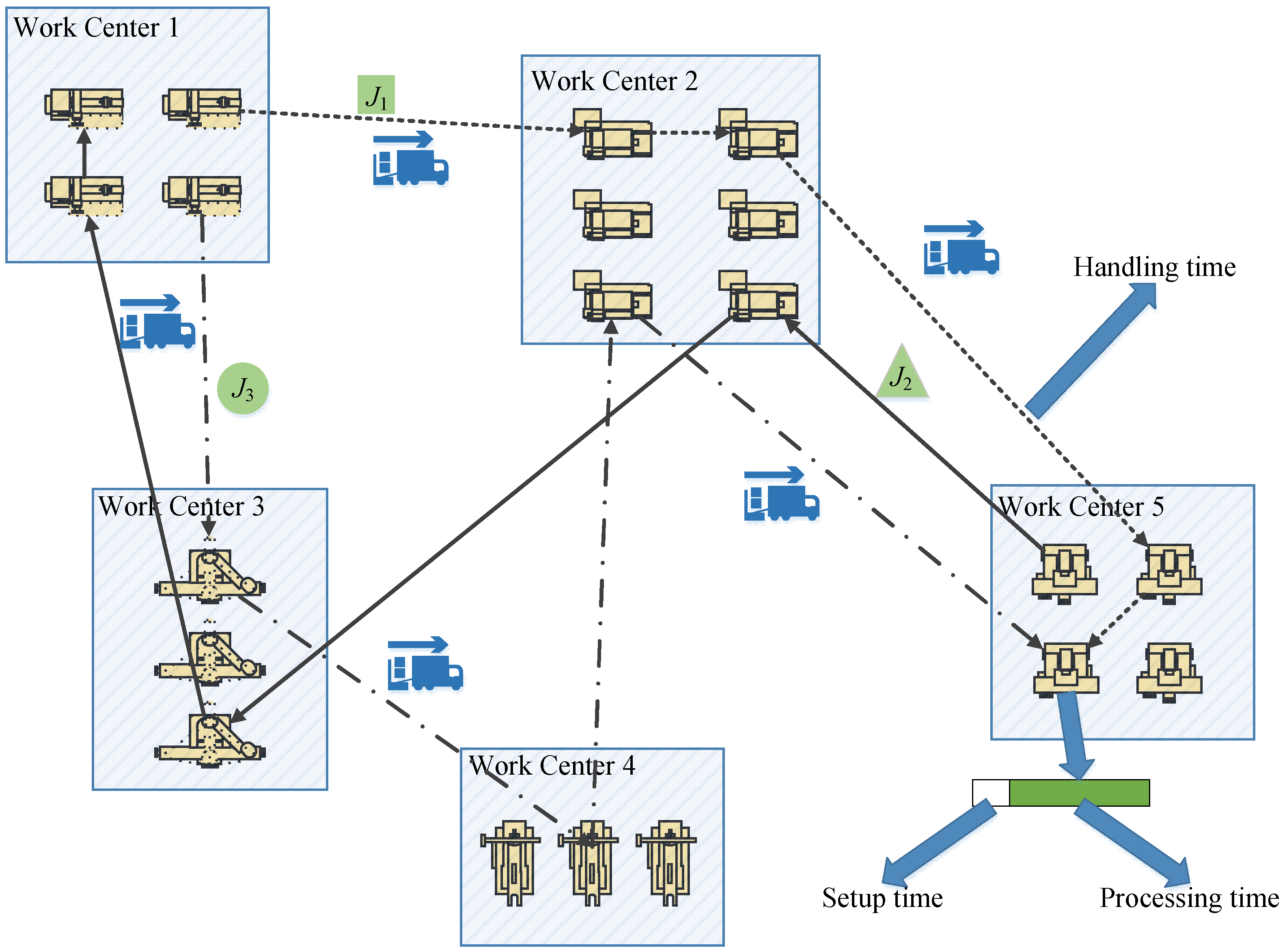
Figure 1. A schematic diagram of the FJSP-cSH.
Applsci 14 04029 g001
Figure 2. Flow chart of the standard SFLA.
Applsci 14 04029 g002
Figure 3. An example of a coding method.
Applsci 14 04029 g003
Figure 4. An example of an operation update.
Applsci 14 04029 g004
Figure 5. An example of a machine update.
Applsci 14 04029 g005
Figure 6. Parallel sequential movement mode.
Applsci 14 04029 g006
Figure 7. Batch handling mode.
Applsci 14 04029 g007
Figure 8. Average effect results under different parameters.
Applsci 14 04029 g008
Figure 9. Gantt chart of optimal scheduling solution for the small practical example.
Applsci 14 04029 g009
Figure 10. Iterative results of the makespan.
Applsci 14 04029 g010
Figure 11. Iterative results of the total number of machine shutdowns.
Applsci 14 04029 g011
Figure 12. Iterative results of the total number of handling batches.
Applsci 14 04029 g012
Figure 13. Gantt chart of optimal scheduling solution for the large example.
Applsci 14 04029 g013
Table 1. The comparison results of different literature.
FJSPTransportationPreparationWork CenterModelAlgorithm
Andy [2]1 CPLNS
Yige et al. [3] RJSPDT
Soroush et al. [4] MILP, CP
Allahverdi et al. [5] FSP, JSP
Zhang et al. [6] DFJSPGEP
Behnke and Geiger [7]
Govi et al. [8] FJSPGA
Pal et al. [9] FJSPhGWO
Feng and Kong [10] HFSP-PSMMNSGA-II-V
This paperFJSP-cSHSFLA-uGSA
1 This represents the consideration of this item in this document.
Table 2. Experimental results of comparison with other algorithms.
Problemα × βSizeLBCCGAGRASPSLGAPSOMSCGASFLA-uGSASD
MK0315 × 81502042042042042042042040
MK0615 × 10150576458697757631.8
MK0720 × 51001391401391441451391442.1
Kacem 014 × 520111111111111110
Kacem 028 × 864141715151415140
Kacem 0310 × 770111313111112110.32
Kacem 0410 × 1010078777770
Kacem 0515 × 10150111213121111120.54
Optimal proportion---25%37.5%37.5%75%62.5%62.5%-
Table 3. Experimental results of comparison between the SFLA-uGSA and the SFLA.
Problemα × βSizeLBSFLA-uGSASFLA
BestAverageSDBestAverageSD
LA0110 × 550570575577.91.88575579.22.61
LA0210 × 550529535541.22.40541543.41.55
LA0310 × 550477477481.73.16482487.04.39
LA0410 × 550502510513.92.10510516.53.94
LA0510 × 550457506514.55.10514520.74.63
LA0615 × 575799799802.31.96801807.14.79
LA0715 × 575749753756.92.70755760.33.11
LA0815 × 5757657667691.807687701.25
LA0915 × 575853856858.81.64858863.93.37
LA1015 × 5758048558582.208678733.85
LA1120 × 5100107110721077.32.7610791084.13.24
LA1220 × 5100936937938.61.40937940.82.15
LA1320 × 5100103810401042.71.6410441046.21.78
LA1420 × 5100107010711073.71.2410711074.42.08
LA1520 × 5100108910941096.72.3810991102.92.46
LA1610 × 10100717728737.19.32735746.28.94
LA1710 × 10100646652657.65.60655661.45.35
LA1810 × 101006637007105.80723730.24.39
LA1910 × 10100617771801.710.16779805.313.85
LA2010 × 101007568008097.20803814.18.32
Table 4. Experimental results with Pareto ranking method.
SinglePareto
12345678910
Target 1204219234209221237213206217204220
Target 23623202121172725243924
Target 311410697107102988689919086
Table 5. Design of job classification.
Job number12345678910
Job type1123333444
Table 6. Design of work center.
Machine number123456
Work center122344
Table 7. Schedule of processing times.
Processing TimesMachine 1Machine 2Machine 3Machine 4Machine 5Machine 6
Job type 1Operation 13- 2--6-
Operation 2--1---
Operation 32-----
Operation 4---66-
Operation 51---65
Job type 2Operation 1-4--6-
Operation 2--4--2
Operation 31---65
Operation 45-4-66
Operation 515----
Job type 3Operation 12---65
Operation 2---26-
Operation 3--12--
Operation 4-35-1-
Operation 5--4--2
Job type 4Operation 1--4--2
Operation 2-44--6
Operation 316---5
Operation 454----
Operation 5-6-6--
2 This operation cannot be processed on this machine. The same meaning as in Table 8.
Table 8. Schedule of setup times.
Setup TimesMachine 1Machine 2Machine 3Machine 4Machine 5Machine 6
Job type 1Operation 11---1-
Operation 2--1---
Operation 32-----
Operation 4---11-
Operation 51---11
Job type 2Operation 1-1--1-
Operation 2--1--1
Operation 32---12
Operation 41-1-11
Operation 521----
Job type 3Operation 11---11
Operation 2---11-
Operation 3--21--
Operation 4-11-2-
Operation 5--1--1
Job type 4Operation 1--2--1
Operation 2-11--1
Operation 321---1
Operation 411----
Operation 5-1-1--
Table 9. Schedule of handling times.
Handling TimesWork Center 1Work Center 2Work Center 3Work Center 4
Work center 1- 3112
Work center 21-11
Work center 311-1
Work center 4211-
3 There is no handling in the same work center.
Table 10. Solution of job scheduling.
Job(i)Operation(ij)Machine(k)Work Center T S i j k B T S i j k T S i j k E / T P i j k B T P i j k T P i j k E
J1O11M5WC401167
O12M3WC210111112
O13M1WC118018220
O14M4WC321122628
O15M1WC128129130
J2O21M1WC1718311
O22M3WC212012113
O23M1WC114216218
O24M5WC423124630
O25M5WC430030636
J3O31M2WC201145
O32M6WC411112214
O33M6WC414014519
O34M6WC419019625
O35M1WC130232133
J4O41M5WC4718614
O42M4WC315015217
O43M4WC317017219
O44M5WC421021122
O45M6WC428028230
J5O51M1WC150527
O52M4WC313013215
O53M4WC319019221
O54M5WC422022123
O55M6WC425126228
J6O61M1WC130325
O62M4WC3819211
O63M3WC213215116
O64M3WC222022527
O65M3WC227027431
J7O71M1WC101123
O72M4WC311011213
O73M3WC216016117
O74M3WC217017522
O75M3WC231031435
J8O81M3WC202246
O82M2WC2516410
O83M1WC120222123
O84M1WC123023528
O85M4WC328129635
J9O91M6WC430325
O92M6WC4505611
O93M1WC111213114
O94M2WC220020424
O95M2WC230030636
J10O10,1M6WC401123
O10,2M3WC2606410
O10,3M2WC210010616
O10,4M2WC216016420
O10,5M2WC224024630
Table 11. Solution of machine scheduling.
Serial
Number
MachineStart Time of Shutdown 3Time of ShutdownCompletion Time of Shutdown
/Start Time of Processing
Time of ProcessingCompletion Time of Processing
1M10003333
2M20003636
3M30003535
4M40882735
5M50001414
6M6147211536
7M60003030
3 The machine from the beginning of time 0 is included in the calculation of a shutdown.
Table 12. Solution of handling scheduling.
Serial
Number
From Work CenterTo Work CenterJobsTime of
Handling
Earliest Start TimeEarliest Completion TimeLatest Start TimeLatest Completion Time
1WC1WC2J2111121112
2WC1WC2J9114151920
3WC1WC3J5, J6, J717889
4WC1WC3J1120212122
5WC1WC3J8128292829
6WC1WC4J2218202224
7WC2WC1J1, J2, J8113141516
8WC2WC4J31561112
9WC3WC1J1128292829
10WC3WC2J6, J7113141415
11WC3WC4J4119202021
12WC3WC4J5121222122
13WC4WC1J9211131113
14WC4WC1J3225273032
15WC4WC2J1013456
16WC4WC2J11781011
17WC4WC3J4114151415
Disclaimer/Publisher’s Note: The statements, opinions and data contained in all publications are solely those of the individual author(s) and contributor(s) and not of MDPI and/or the editor(s). MDPI and/or the editor(s) disclaim responsibility for any injury to people or property resulting from any ideas, methods, instructions or products referred to in the content.