Featured Application
The new algorithm proposed in this paper is mainly applied to radar data processing. By accurately distinguishing between targets and clutter, the clutter removal rate can be improved, and target trajectories can be quickly and accurately established. This algorithm can comprehensively utilize the advantages of classifiers and data characteristics, reducing the dependence on training samples. Therefore, it is also suitable for classification applications on small sample datasets.
Abstract
Accurately classifying targets and clutter plots is crucial in radar data processing. It is beneficial for filtering out a large amount of clutters and improving the track initiation speed and tracking accuracy of real targets. However, in practical applications, this problem becomes difficult due to complex electromagnetic environments such as cloud and rain clutter, sea clutter, and strong ground clutter. This has led to poor performance of some commonly used radar plot classification algorithms. In order to solve this problem and further improve classification accuracy, the radar plot classification algorithm based on evidence adaptive updating (RPC-EAU) is proposed in this paper. Firstly, the multi-dimensional recognition features of radar plots used for classification are established. Secondly, the construction and combination of mass functions based on feature sample distribution are designed. Then, a confidence network classifier containing an uncertain class was designed, and an iterative update strategy for it was provided. Finally, several experiments based on synthetic and real radar plots were presented. The results show that RPC-EAU can effectively improve the radar plot classification performance, achieving a classification accuracy of about 0.96 and a clutter removal rate of 0.95. Compared with some traditional radar pattern recognition algorithms, it can improve by 1 to 10 percentage points. The target loss rate of RPC-EAU is also the lowest, only about 0.02, which is about one third to one half of the comparison algorithms. In addition, RPC-EAU avoids clustering all radar points in each update, greatly saving the computational time. The proposed algorithm has the characteristics of high classification accuracy, low target loss rate, and less computational time. Therefore, it is suitable for radar data processing with high timeliness requirements and multiple radar plots.
1. Introduction
Radar is an important tool for remote detection and tracking of targets, with significant applications in both military and civil fields. Radar emits electromagnetic wave energy into a certain direction in space and receives echoes reflected by objects in that direction, thereby discovering and determining targets. In the actual detection of radar, in addition to the real target echo, the received echo also contains much cloud and rain clutter, sea clutter, and ground clutter. Cloud and rain clutter refers to the abnormal clutter caused by the reflection of radar beams by clouds and rain. Sea clutter refers to the backscattered echoes of the sea surface under radar illumination. Ground clutter refers to ground echoes caused by the super-refraction of radar beams. The characteristics of these mixed clutters are complex and irregular, which will increase the difficulty of identifying real targets. Under the processing of existing target detection methods, clutter cannot be completely eliminated. Therefore, determining whether a target is true or false in a cluttered background is also a basic task in radar data processing [1,2,3]. These large numbers of clutter plots will have two impacts on subsequent radar data processing. First, they can generate a large number of false trajectories, making it difficult to accurately track real targets. In addition, they will inevitably waste computing resources and affect the processing efficiency of the system. Therefore, it is necessary to further classify the target and clutter after object detection and to filter out a large number of false clutter plots that affect radar data processing.
In order to effectively achieve accurate classification of targets and clutter plots, some scholars have conducted a series of studies [4,5,6,7]. In [5,7], the radar plot classification methods based on an optimized support vector machine were proposed, which achieved the distinction between targets and clutter by extracting echo features and fusing multiple features. In [4], Lin et al. used a weighted KNN model to identify the authenticity of radar plots. In [6], Sun et al. proposed a false plot identification method based on multi-frame clustering. These methods are limited to certain scenarios, and the recognition results are not good enough. In recent years, the development and application of artificial intelligence algorithms, especially deep learning network models, have provided a lot of help in solving problems. So, in the field of radar point data processing, fully connected neural networks [8,9], convolutional neural networks [10,11,12], recurrent neural networks [13], multi-layer perceptron [14,15], and their variations or combinations with other algorithms [16,17], have been widely studied. Due to their better feature extraction ability, they can improve the classification accuracy to a certain extent, reaching over 90%. However, due to the lack of representation of uncertain information, they can only make hard judgments of yes or no. But in many specific applications, multi-step decision-making is required. Initially, uncertain classifications can be retained, and then accurate classification can be gradually achieved based on supplementary evidence information.
In order to effectively represent and process uncertain and imprecise information, the belief function theory has been proposed and developed [18,19,20]. At first, it was mainly used to achieve the fusion of multi-sensor data, but later it was expanded to many applications by some scholars. These applications mainly include pattern classification [21,22,23,24,25,26], evidential clustering [27,28,29,30,31,32], multi-sensor data fusion [33], decision making [34,35], image segmentation [36,37], security assessment [38,39], abnormal condition detection [40], and user preference analysis [41,42]. The confidence function has been fully proven to be effective in many fields. Considering that identifying targets and clutter in radar plots is essentially a data classification problem, combining belief functions with deep learning networks to improve classification accuracy is a meaningful topic. Therefore, we proposed the radar plot recognition algorithm based on adaptive evidence classification (RPREC) [43,44], which effectively improves the classification accuracy of radar plots. The limitation of RPREC is that the classifier needs to be retrained during each iteration process. This consumes a lot of computing time and is not conducive to the applications that pursue timeliness. But the iterative updates adopted by RPREC provide us with a good idea for researching the new algorithms in this paper. Therefore, in order to further improve the classification accuracy, and also to effectively shorten the calculation time, the radar plot classification algorithm based on evidence adaptive updating (RPC-EAU) is proposed in this paper. It mainly consists of three parts. Firstly, we establish multi-dimensional features of radar plots that can be used to distinguish between targets and clutter. Secondly, based on the distribution of samples in the feature space, the mass function was constructed, optimized, and combined. Then, we designed a confidence network classifier based on deep learning, which can give confidence that any radar plot belongs to the target, clutter, and uncertain classes. Finally, an iterative update strategy for the evidences and confidence classifier was established. When there is no significant difference in the judgment between the classifier and the combined evidence, the classification result is directly output. When there are certain differences, the evidence is corrected and the classifier is optimized. The optimized classifier then continues to classify radar plots that are difficult to distinguish. It can be seen that RPC-EAU fully utilizes a collaborative decision-making strategy based on classifiers and data distribution, which not only ensures efficient output of easily classified radar plots, but also ensures multi-step optimization decision making for difficult-to-classify plots. So, while improving classification accuracy, it is also possible to minimize computation time and ensure the efficiency performance of the model. Several experiments based on synthetic and real radar plots show that proposed RPC-EAU algorithm performs better than some typical radar plot classification methods. RPC-EAU not only improves classification accuracy, but also reduces the number of iterations to achieve low computation time. The statistical results show that it can achieve a classification accuracy of around 0.95 while maintaining a target loss rate below 0.02. The CPU time is about 2 to 4 s, which is at the same level as deep network recognition algorithms. Although these studies are exciting and interesting, there are still some studies worth further investigation, such as the adaptive setting of some parameters in algorithms.
The rest of this paper is organized as follows. In Section 2, we will recall the belief functions, evidence classification and the intelligent radar plot classification, respectively. In Section 3, we will introduce the proposed radar plot classification algorithm based on evidence adaptive updating. Finally, several experiments based on synthetic and real radar plots will be presented in Section 4, and the paper will be concluded in Section 5.
2. Related Work
2.1. Belief Functions
The belief function theory, also known as evidence theory, has been proven to be highly effective in handling uncertain and imprecise information.
In belief functions, a problem domain is represented by a finite set called the frame of discernment. The set of all subsets of is called the power set of and is denoted . is an independent event under the discernment frame . The combination results of all subsets of are included in . For example, if , then .
is an empty set, representing an impossible event with a confidence assignment of 0. represents complete lack of knowledge and uncertainty as to which independent event occurred. The mass function is used to represent the degree support for each element from . It satisfies a mapping relationship from to [0, 1], such that:
The subsets are called the focal elements of . If , then . And the sum of the basic assignments of all nonempty subsets is 1.
For the subset , the belief function represents the probability that the evidence supports its validity. The belief function can be defined as the following equation.
The plausibility function represents the probability that the evidence does not contradict , and can be defined by the following equation.
In order to provide readers with a clear understanding of the meanings of and , Figure 1 is presented as follows.

Figure 1.
The relationship between Bel and Pl in belief functions.
For example, we are certain that the probability of event occurring is 0.5 and the probability of its not occurring is 0.2. Then, we will obtain the results that , , , .
The combination of different pieces of evidence plays an important role in belief functions. Assuming that and are two independent pieces of evidence to be fused, represents the various propositions provided by Evidence 1, and represents the various propositions provided by Evidence 2. is obtained through the intersection operation of and , which represents the various propositions of the combined evidence. The combination of and with Dempster’s (D-S) rule is defined by:
where
For the nonempty , where represents the degree of conflict between and , such that , if the value of is close to 1, indicating a high conflict between the two pieces of evidences, the D-S rule will have certain shortcomings. To deal with this problem, some improvement rules have been studied. The most representative one among them is the Yager rule, which can assign the degree of conflict set as uncertain by the following combined formula.
In addition, there are many other improvement rules, such as Smets, Dubois and Prade, PCR5, DSmT, and so on. Although these improved rules solve the problem of high conflict allocation when combining evidences, the convergence speed of the algorithm is not as fast as D-S. Therefore, it is necessary to make reasonable choices based on specific tasks and even using multiple combination rules.
2.2. Evidence Classification
In the field of pattern classification, evidence classification algorithms have significant advantages over traditional classification algorithms in representing uncertain information and can effectively improve classification accuracy. The key to implementing evidence classification lies in the construction and combination of decision evidence, and the basic principles of its implementation are as follows.
Assuming an object needs to be divided into a certain class in the category set of . Here, represents the total number of pattern categories. Let be the training set with samples. is the class label of sample . It is necessary to select a certain number of samples from this training dataset to construct evidence, which can be used to assist decision making. There are many ways to select samples, but random selection and selecting nearest neighbors based on feature distance are the two most commonly used methods.
Suppose that is the jth nearest neighbor sample of the object , with a class label of . Here, , is a specific value that can be obtained from training samples. The decision evidence constructed through can be described by Equation (7).
where is the confidence that belonging to class , and represents the uncertainty about the class of . is the feature distance between and . is a mapping function that can convert the feature distance to the interval . In [21], it was proposed toto be set as:
The parameter can be heuristically set as 0.9 to 0.95, and is usually selected as 1 or 2. After obtaining the evidences of nearest neighbors in sequence, the next step is to combine them using the Dempster–Shafer rule.
The class label of can be determined by the global mass function . We can then assign object to the class with the highest confidence.
2.3. Intelligent Radar Plot Classification
In radar data processing, a large number of clutter plots surround the real target, which increases the difficulty of accurate classification. Traditional methods for judging truth from falsehood are difficult to use to fully characterize the distinguishing rules of sample features. The birth and development of artificial neural networks have provided great support for solving this problem. Therefore, some radar plot recognition algorithms based on neural networks have been studied by experts and scholars.
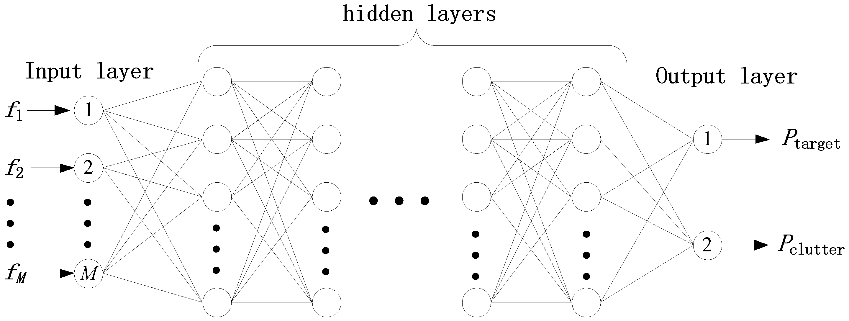
A fully connected neural network, also known as a feedforward neural network, is the most basic type of artificial neural network. In this network, neurons (or nodes) are organized into multiple layers, with each layer’s neurons connected to both the previous and subsequent layers, but there is no connection between neurons within the same layer. The data propagates unidirectionally from the input layer to the output layer without feedback (or loop) connections. Each connection of a fully connected neural network has a weight, which is learned through training data. Each neuron calculates the weighted sum of all its inputs, and then obtains its output through an activation function such as ReLU, sigmoid, or tanh. The fully connected network structure for radar block classification is shown in Figure 2.

Figure 2.
The fully connected network structure for radar plot classification.
Input layer: The number of nodes in this input layer depends on the feature dimension of the radar data. For example, assuming the input feature is , the number of input nodes needs to be set to .
Hidden layer: The design of network hidden layers is usually related to two factors, the size of radar plots and the spatial distribution of feature data. There are no specific rules to follow, and usually exploratory experiments are used to guide the design.
Output layer: The number of nodes in the output layer is generally set to 2, corresponding to the probabilities of being the target and clutter, respectively. Using to represent the probability that the radar point is the target, and to represent the probability of clutter, they satisfy the relationship .
Fully connected neural networks have many advantages, such as an intuitive structure, high computational efficiency, and convenient configuration. Therefore, the research on its application in radar plots is very valuable.
3. Proposed Method
In this section, the radar plot classification algorithm based on evidence adaptive updating (RPC-EAU) is presented in detail. The feature extraction of radar plots will first be described in Section 3.1. The construction and combination of mass functions based on feature sample distribution are presented in Section 3.1 and Section 3.2, respectively. The design and iterative update strategy of confidence network classifiers are discussed in Section 3.4. Finally, the evaluation indicators for the RPC-EAU are provided in Section 3.5.
3.1. Radar Plots Feature Extraction
For a classification problem, the first thing to focus on is reasonable feature selection. We selected range, azimuth, elevation, distance width, azimuth width, total number of resolution units, maximum amplitude, minimum amplitude, average amplitude, and number of resolution units exceeding the threshold as the 10 dimensional recognition features of the radar plots. The design of the extracted features here refers to those features mentioned in [8,9,16]. The specific meanings about these features are shown in Table 1.

Table 1.
The extracted features and their meanings.
There is a significant difference in the range of different sub-features of radar plots. Normalization can eliminate dimensional differences between different sub-features, making them comparable and improving the performance of the model. Therefore, the extracted original feature is normalized by the following formula.
Here, represents the sub-feature of , whose dimension is . and are the maximum and minimum values that can be taken for this sub-feature, respectively. is the qth dimensional sub-feature obtained by normalization, with a value interval of [0, 1].
3.2. Construction of Belief Function
In belief function classification, the most important thing is to construct a reasonable mass function for each decision evidence. Consider a radar plot classification problem in which the objects have to be classified into a certain class from . Here, and represent the target and clutter, respectively. While represents the uncertain class, the samples within it need to be further divided into and by additional information.
Firstly, we need to use the feature extraction method in Section 3.1 to obtain the features of these radar plots. And the feature set of these radar plots can be obtained. Then, we calculate the feature distance between each radar plot using the following formula.
where represents the qth dimensional feature of targets and , with values ranging from 1 to 10. Here, is the Euclidean distance between and . After pairwise calculations of all radar plots, the following symmetric feature distance matrix can be obtained.
The reason why the elements of the main diagonal of matrix D have values of 0 is that they represent the distance between the sample and itself. The information contained in this feature distance matrix can be used to guide us in constructing decision evidences. A very effective strategy is to select other neighbors near a certain radar plot to be achieved.
Assuming we construct the mass function of , and is the set of nearest neighbor samples obtained from the feature distance matrix . Support that the class label of neighboring sample is . Then, the mass function constructed by on can be defined as the following formula.
Here, is the confidence level that considers to belong to class ; therefore, the value of ranges from 0 to 1. Then, the key is to convert to the value interval through a certain mapping function. We find the maximum feature distance and the minimum feature distance of K-nearest neighbor samples as follows:
We then modify the feature distance of each neighboring sample based on the maximum and minimum values of these feature distances.
Many attempts have been made in the design of mapping functions such that , and exponential functions have been proven to be the most suitable. Therefore, the mapping function in this paper is defined as:
Here, parameter is a fixed value used to adjust the mapping, which can be heuristically set to 2. The parameter is related to the distribution of K-nearest neighbor samples in the feature space. And the value of the parameter is usually selected as 1 or 2.
Through the above methods, the mass functions of K pieces of evidence for can be obtained sequentially. In the same way, decision evidence for all radar plots can also be constructed.
In order to better demonstrate the process of constructing the mass function of radar plots, a numerical example is given below.
Example 1.

To construct some decision evidences for a certain radar plot , where , , and are four neighboring samples selected in the feature space. Their feature distances from are as follows:
Then, we traverse to search for the maximum and minimum distances, and obtain:
Correcting each feature distance, one obtains:
The mapping correction parameter of target can be calculated as:
Then, we need to obtain the support of each neighboring evidence through Formula (18):
Finally, based on the class labels of each neighboring evidence, the mass function of can be constructed. The class labels for both and are assumed to be , indicating that they can provide confidence that is target. The class label of is , indicating that it can provide confidence that is clutter. The class label of is , indicating that it knows nothing about the target and cannot provide any valuable classification information. Here, #1, #2, #3 and #4 are used to represent the evidence of the four nearest neighbors, respectively. And the specific results of the mass function constructed by each nearest neighbor are shown in Table 2.

Table 2.
The mass function constructed by different nearest neighbor samples in Example 1.
3.3. Correction and Combination of Evidences
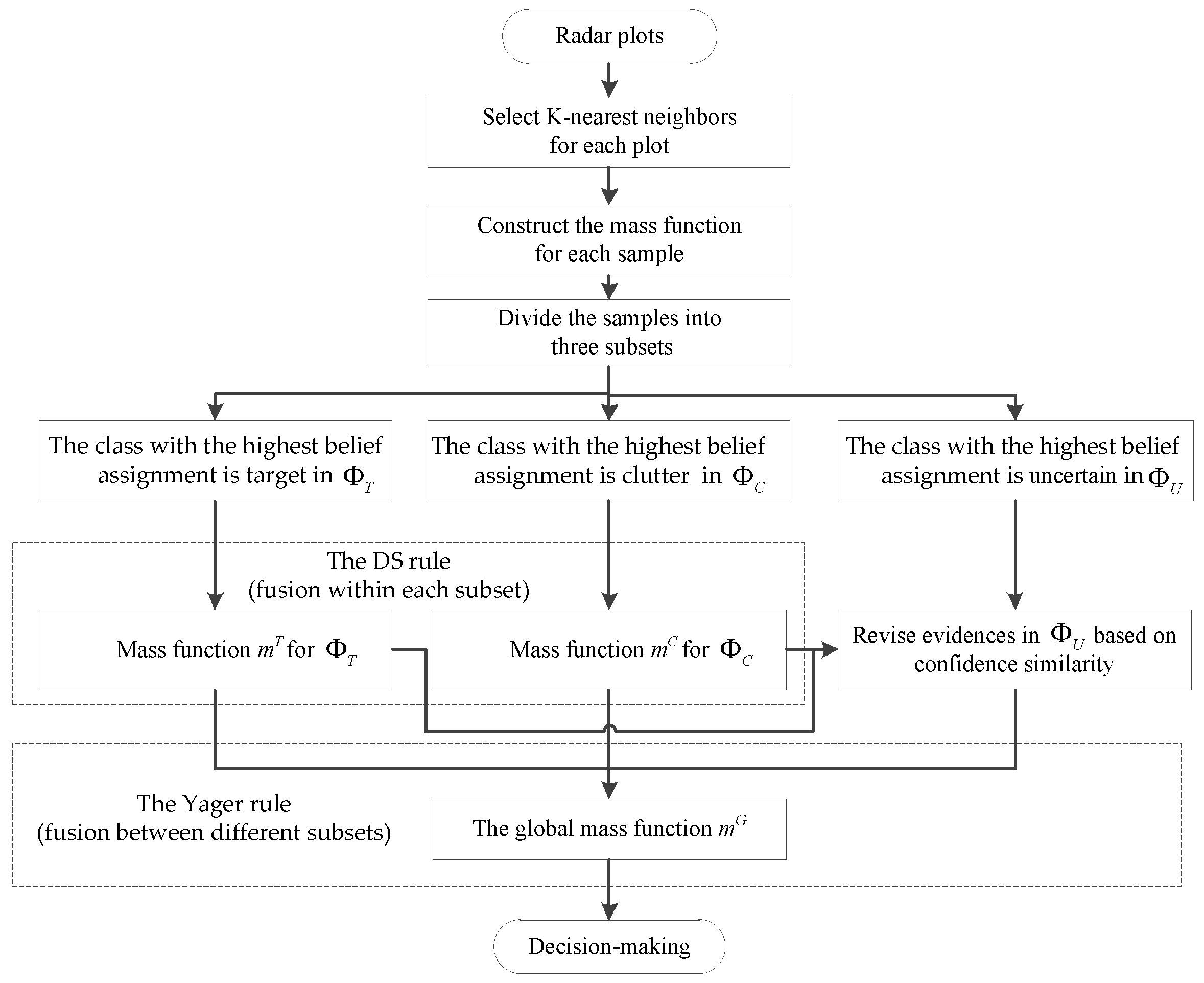
Although each neighbor sample evidence can provide some decision information for radar plot classification, it is particularly important to effectively combine them when these pieces of evidence are not completely consistent. In this section, a specific mixing combination rule is developed to fusion mass functions of the evidences about radar plots. This rule can be referred to as the “D-S + Yager” rule, which can have the efficiency of D-S when processing evidences in the same group, while also having the rationality of Yager in conflict allocation when processing evidences between different groups. For a sample set with K-nearest neighbor evidence, the evidence correction and combination based on this rule are as follows:
Step 1: According to the maximum confidence corresponding to target, clutter, or uncertainty, K-nearest neighbor evidence can mainly be divided into three subsets , and , where , and . The number of evidences contained in them is , , and .
Step 2: There is no conflict between the mass functions in this same set. Therefore, the D-S rule can be chosen to combine the evidences in or separately. We use and to represent the combined mass functions, and they are defined as follows:
And
The reason why the evidences in subset are not directly combined in this step is that they assigned all confidence to unknown, which results in the combination not providing effective decision information.
Step 3: Then, we need to combine and , but there may be some conflicts between them, since, compared to the D-S rule, the Yager rule can perform better when combining these conflicting evidences. So, it is chosen at this step to fuse the conflicting mass function in sets and obtained in the previous step. The combined mass functions obtained by and are given by:
Step 4: The evidences in have the relationship that . So, combining them without correction does not provide additional decision-making information. Therefore, it is necessary to modify these evidences based on and , which can be seen as the fused confidence center of and . Here, is used to represent the confidence similarity between and , and is used to represent the confidence similarity between and , defined as:
Then, we also use the number of evidences as a discount factor, and the updated mass functions for each class from can be obtained as:
Step 5: The Yager rule is still used to combine and , so that the global mass function can be obtained by:
Each radar plot can form its own global mass function through the above steps. In a sense, these mass functions reflect the confidence distribution in the feature space between different radar plots. This is very helpful for the design and updating of classifiers in the following section of this paper.
The correction and combination of evidences discussed above is summarized as a flowchart in Figure 3.

Figure 3.
Flowchart of the correction and combination of evidences in the proposed method.
To better illustrate the combination of K nearest neighbor evidences, an example is given below.
Example 2.


Assume there are six pieces of nearest neighbor evidence. We need to combine them to give a decision on the class to which the object belongs. For simplicity, we use #1, #2, #3, #4, #5, and #6 to represent them sequentially. Evidences #1 and #3 suggest that the object may belong to class ; therefore, they provide confidence levels of 0.8 and 0.9 for class , respectively. On the contrary, evidences #2, #4, and #5 suggest that the object may belong to class , therefore giving the confidence levels of 0.5, 0.4, and 0.2 for class , respectively. Evidence #6 does not provide any information about the target class; therefore, all confidence is given to the unknown. The specific mass function representations of these six pieces of nearest neighbor evidence are shown in Table 3. According to the combination process in the proposed method, evidences belonging to the same class are first combined based on the D-S rule—that is, combining #1 and #3 to obtain , as well as #2, #4 and #5 to obtain ; then, combining and to obtain by using the Yager rule, while also correcting #6 based on them. Finally, the global mass function is obtained by fusing with the modified evidence . The results obtained from these steps are shown in Table 4.

Table 3.
Evidence needs to be combined in Example 2.

Table 4.
The results obtained by combining evidences from each step.
3.4. Design and Update of Confidence Classification Network
In traditional typical radar plot recognition algorithms, the binary classification is widely studied. These algorithms are rapid and simple in determining whether a certain radar plot is target or clutter in [3,4,5,6,7]. Of course, such rapid decision making inevitably increases some misjudgments. So, we added an uncertain class to this radar plot classification problem by drawing on the concept of belief functions. In this way, radar plots that are difficult to make decisions can be first classified as uncertain. Then, through further in-depth data feature analysis or classifier optimization, more reasonable judgments can be made. Therefore, the classifier design and optimization in the proposed algorithm are presented in detail here.
3.4.1. Classifier Design
Deep learning networks have unique advantages in data classification. They can extract the deep characteristics of samples through layer-by-layer networks, thereby achieving the separation in high-dimensional feature spaces. Considering that radar plots do not have the same complexity as image information, it is not necessary to use complex network structures such as convolutional neural networks and recurrent neural networks. Therefore, a fully connected neural network with more efficient uncertain data processing capabilities is designed in this paper.
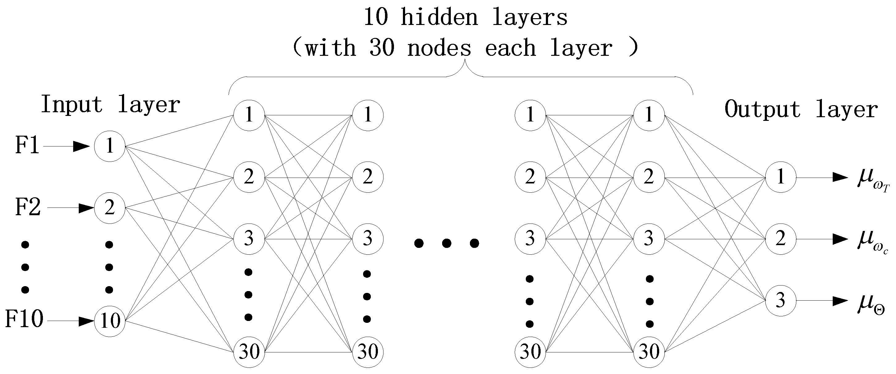
The specific design of this confidence classification network is shown in Figure 4. Firstly, the radar plot features are received through the input layer. Then, deep feature mining is carried out through hidden layers. Finally, in the output layer, the membership degree of radar plots belonging to target, clutter, and uncertainty is given. The specific parameter configurations for each layer of this confidence classification network are as follows:
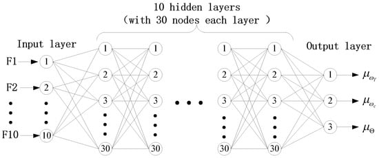
Figure 4.
The design of confidence classification network for radar plots.
Input layer: Before being entered into the confidence network classifier, all radar plots need to undergo feature extraction and normalization processing as described in Section 3.1. Therefore, the number of input layer nodes corresponds to the dimension of normalized features, which is set to 10.
Hidden layer: The design of hidden layers usually considers two factors: the size of radar plots and the distribution of samples in the feature space. After some exploratory data analysis experiments in the early stage, setting the hidden layer at 10 layers with 30 nodes in each layer has a good effect. ReLU, Sigmoid, and Tanh functions are the most commonly used activation functions. ReLU has a fast convergence speed, so it is chosen to activate each hidden layer.
Output layer: In the output layer, it is necessary to provide the membership degree of radar plots belonging to target, clutter, and uncertainty. So, the number of output layer nodes is set to three. We use , , and to represent the class membership, which can be seen as the probability that each radar plot belongs to target, clutter, and uncertainty. They satisfy the relationship that .
3.4.2. Classifier Optimization
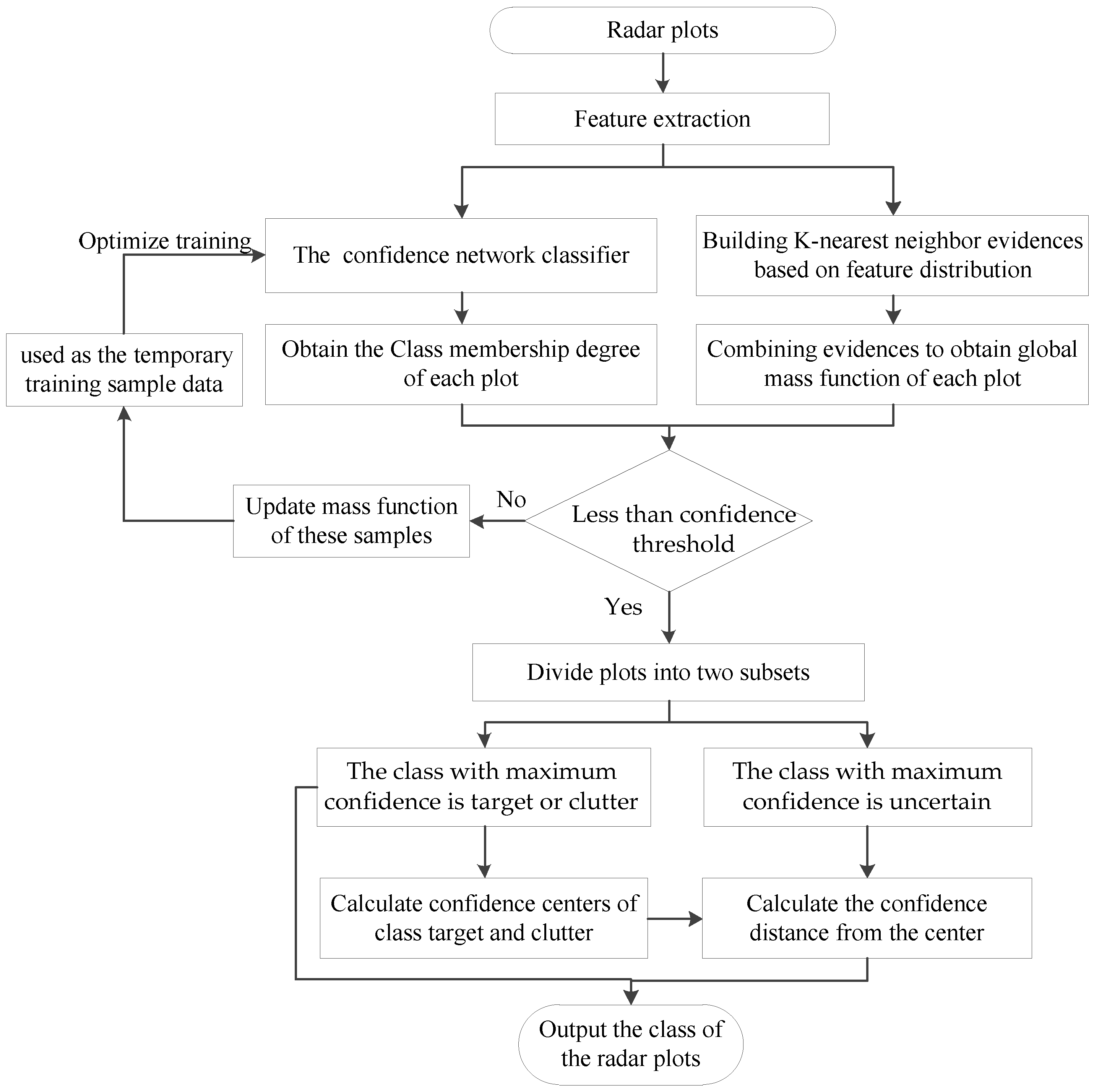
Let be the training set with samples. Firstly, we perform offline initial training on the confidence classification network based on the training sample set . Assuming is a dataset of radar plots to be classified, after extracting features from all these radar plots, the following process is performed as follows:
Step 1: The trained confidence network classifier is used to obtain the class membership of these samples. The class membership of each sample can be expressed as , satisfying the following equation. Since the classifier’s outputs only contain three classes—target, clutter, and uncertainty—the value of is 3.
Step 2: Select K-nearest neighbor samples based on the intrinsic feature distribution of these radar plots. As shown in Section 3.1 and Section 3.2, construct and combine evidence to obtain the global mass function for each sample such that .
Step 3: Calculate the confidence distances between and of each sample using the following equation.
Step 4: When is less than a certain threshold represented by , it indicates that the classifier has good consistency with the data distribution results. These samples can be divided into two subsets which are defined as follows:
The classification results of the samples in subset can be direct output, which gives a judgment on whether the sample is target or clutter. At the same time, these samples are also used to provide decision assistance to subset . Then, the center of these classes can be obtained as follows.
For the samples in subset , we calculate their confidence distances from the class center and separately and assign these samples to the class with the minimum confidence distance in sequence.
Step 5: When is bigger than the threshold , it indicates that the classifier and data distribution have different perceptions of samples’ confidence. Then, we need to make the following evidence correction.
Here, is the confidence correction factor, which is usually set to 0.5 if there is not much experience to follow.
Step 6: These corrected evidences are used as temporary samples to optimize the confidence network classifier.
Step 7: For the samples obtained in step 5 that are greater than the confidence threshold, we repeat steps 1 to 6 based on the optimized confidence network classifier.
Step 8: A certain number of samples are accurately classified in each iteration update. Therefore, we stop the iterative optimization process until no samples exceed the confidence threshold. Then, all the samples are accurately classified.
From the above process, it can be seen that the confidence classification network in the proposed algorithm has two advantages. Firstly, it can quickly provide classification results for easily distinguishable samples, which can also provide decision support for uncertain samples. Secondly, K-nearest neighbor evidence can be constructed based on the distribution of radar plots, which can iteratively optimize the confidence classification network and provide more accurate classification results.
In RPC-EAU, the iterative update process for the class labels of radar plot is shown in Figure 5.

Figure 5.
The flowchart for updating class labels of radar plots.
3.5. Algorithm Performance Evaluation
In RPC-EAU, the classification accuracy, target loss rate and clutter removal rate are used to evaluate its effectiveness. For ease of use, they are represented by , , and , respectively.
The classification accuracy is the proportion of correct radar plots identified by this algorithm model, defined as follows:
Here, and represent the target and clutter plots that can be correctly classified, while and represent the targets and clutters that have been misclassified as each other, respectively.
In practical applications, losing the target plots can sometimes lead to serious impacts, even far higher than the loss of identifying clutter as target. Therefore, it is necessary to consider the target loss rate as an important evaluation indicator. Its definition formula is as follows:
While ensuring that the target plots are not misclassified, it is important to recognize as much clutter as possible for filtering. So, the clutter removal rate is used as another important evaluation indicator, defined as the following formula:
The procedure is summarized in Algorithm 1.
| Algorithm 1 RPC-EAU algorithm |
| Require: Radar plots set ; training set ; confidence threshold ; number of decision evidences K; confidence network classifier; Initialization: The initial offline training of the confidence classification network is carried out based on this training set. 1: Extract features from each radar plot in set . 2: t ← 0; 3: Repeat 4: Obtain the class membership of each sample based on the confidence classification network. 5: Select K-nearest neighbor samples based on the feature distribution of these samples. Construct and combine evidences to obtain the global mass function for each sample . 6: Calculate the confidence distance between and of each sample. 7: Divide the samples with a confidence distance less than the confidence threshold into two subsets and . 8: Output the classification results of the samples in subset . At the same time, calculate the class centers of these samples. 9: For the samples in subset , calculate their confidence distances from the class center and separately. 10: Assign the samples to the class with the minimum confidence distance in sequence. 11: For those remaining samples whose confidence distance is greater than the threshold , correct their evidences using Equation (35). 12: Optimize training confidence network classifiers by using these modified evidences. 13: t ← t + 1. 14: until there are no samples with confidence distance exceeding threshold . 15: return the class labels of each radar plot. |
4. Experiments
In this section, several experiments based on radar simulation plots and real plots are presented. Firstly, an artificial sample set for these experiment was constructed based on the results of the radar processing program in Section 4.1. In Section 4.2, the effectiveness of the proposed RPC-EAU was evaluated through comparison with some typical radar plot recognition algorithms. Then, the parameter analysis of the RPC-EAU was provided in Section 4.3. Finally, in Section 4.4, the effectiveness of RPC-EAU was also validated in a practical application example.
These experiments were conducted on the Lenovo Legion Y9000P, which has an Intel(R) Core(TM) i9-14900HX CPU @2.5 GHz and 32 GB MEMORY. All these comparison algorithms are implemented based on MATLAB code and executed in MATLAB R2023b under the Windows 11 system.
4.1. Synthetic Dataset
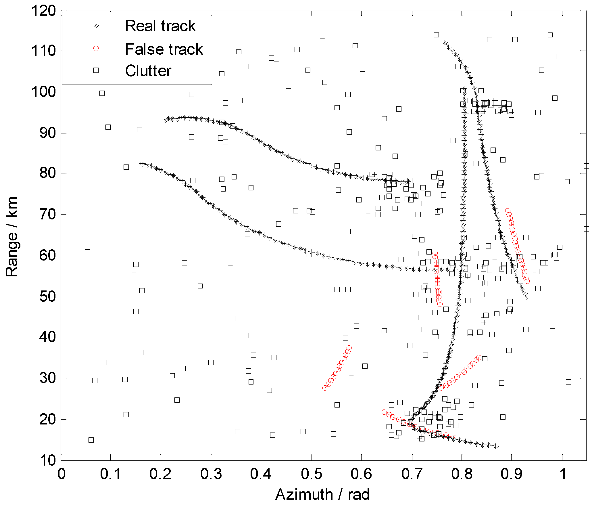
The experimental data come from the X-type sea monitoring and tracking radar. But these data have already been processed by radar tracking programs. So, most of the clutter plots have been filtered out, resulting in the experimental data mainly consisting of three parts: real target trajectory, false trajectory, and some remaining clutter plots. The distribution of the experimental dataset is shown in Figure 6.

Figure 6.
The distribution of the experimental dataset.
Firstly, mark the radar plots corresponding to the real trajectory as targets. Then, mark the radar plots associated with false trajectories as uncertain. Finally, record all remaining plots as clutter. As shown in Table 5, there are 372 targets, 263 clutters, and 86 uncertain samples in the constructed sample set.

Table 5.
The number of samples in each class.
4.2. Classification Performance
This experiment is mainly used to verify the classification performance of RPC-EAU, which is based on the sample set constructed in Section 4.1. Meanwhile, we compared various typical radar plot recognition algorithms, which are not only based on traditional machine learning but also on deep learning. These typical radar plot recognition algorithms mainly include PSO-SVM [5], IKNN [4], RPC-FNN [9], RPC-RNN [13] and RPREC [43]. In this experiment, the parameter settings of these algorithms still follow the settings from their respective references. The difference is that the input features of all algorithms are replaced with the 10 dimensional features set in this paper, such that the nearest neighbor parameter of IKNN is still set to 7. In the PSO-SVM, the optimal combination of kernel function and error penalty factor is selected as 15 and 22. The RPC-FNN adopts a five-layer network structure, with nodes in each layer being 10, 64, 128, 32, and 2, respectively. RPC-RNN adopts the complex network structure of 100 hidden layers as described in the reference. In the RPREC, the number of iterations is set to 1000, and the confidence threshold parameters T1 and T2 are selected as 0.4 and 0.1, respectively. In the proposed algorithm RPC-EAU, the parameter K representing the number of nearest neighbor decision evidences is set to 8, and the confidence threshold parameter is set to 0.2.
In order to eliminate the impact of sample selection, we conducted three independent experiments, randomly selecting half of the samples for training and testing the remaining ones each time. The specific situation of the samples selected in these three experiments is shown in Table 6. The classification accuracy, target loss rate and clutter removal rate that are designed in Section 3.5 are used to evaluate the effectiveness of the algorithms. At the same time, in order to verify the timeliness of these algorithms, the CPU time was also recorded in the experiment. The average results of three experiments on these indicators are recorded in Table 7. The , , and are, respectively, used to represent the classification accuracy, target loss rate, clutter removal rate and CPU time.

Table 6.
The number of training and test samples in each experiment.

Table 7.
The average results of these three experiments.
The experimental results in Table 7 show that the radar plot classification algorithms PSO-SVM and IKNN based on traditional machine learning have the shortest CPU time, both within 1 s. However, their classification accuracy and clutter removal rate are also the lowest, generally in the range of 0.83 to 0.87, with a target loss rate of about 0.12. Compared to PSO-SVM and IKNN, the algorithms RPC-FNN and RPC-FNN based on deep learning improved the classification accuracy and clutter removal rate, reaching around 0.91. At the same time, the target loss rate decreased to below 0.06, but the CPU time also increased by two to five times. RPREC has the advantages of deep learning and evidence clustering. Compared to RPC-FNN and RPC-RNN, the classification accuracy and clutter removal rate can be improved by about 3 percentage points. The target loss rate has also been reduced by more than half. But the cost is a huge CPU time, increased by more than 10 times to 24.21 s. The proposed algorithm RPC-EAU has a similar target loss rate compared to RPREC, with slightly improved classification accuracy and clutter removal rate. But the CPU time has significantly reduced to 2.87 s; although not as fast as PSO-SVM and IKNN, it can still maintain the same level of CPU time as RPC-FNN and RPC-RNN. Compared with other radar plot recognition algorithms in this experiment, RPC-EAU has the highest classification accuracy and clutter removal rate, as well as the lowest target loss rate. The CPU time of RPC-EAU is also moderate.
Therefore, it can be seen that traditional radar plot classification algorithms based on machine learning are the most efficient in terms of computational speed, but their drawback is that the distinction between targets and clutters is not accurate enough. The radar plot classification algorithm based on deep learning can extract more refined features through complex networks, thereby obtaining better discrimination between targets and clutters. RPREC can fully utilize the distribution characteristics of online radar plots and iteratively optimize the network classifier to achieve high classification accuracy. However, each round of clustering analysis and classifier retraining will generate a lot of computational time.
The proposed RPC-EAU algorithm fully utilizes the collaborative decision-making strategy based on classifier and data distribution, which quickly outputs mutually assured results and comprehensively optimizes uncertain data. This not only improves classification accuracy but also reduces the number of iterations to achieve low computational time.
4.3. Parameter Analysis
In the RPC-EAU, the number of nearest neighbor decision evidences and the confidence threshold are two crucial parameters that have a significant impact on performance. The parameter reflects the number of samples distributed around the object in the feature space. So the larger the value, the richer the decision information will be. The parameter represents our tolerance for the difference between the results given by the classifier and those obtained based on radar plot distribution.
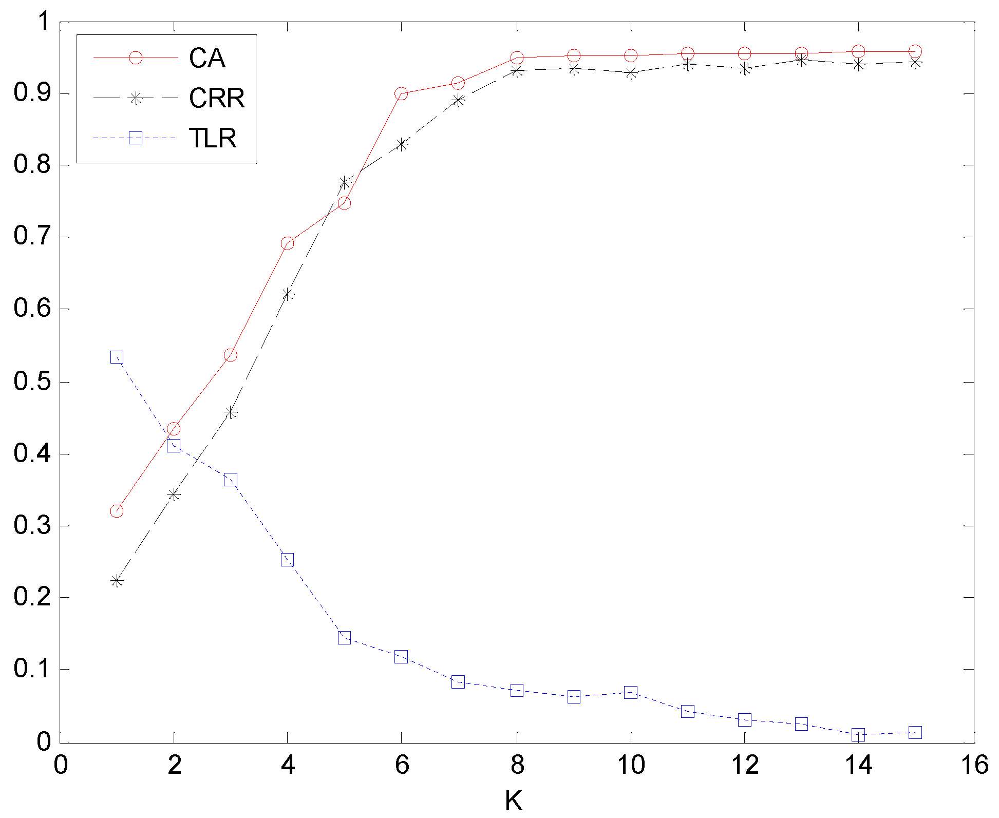
Therefore, the roles of and were analyzed in detail in this experiment. The , , and of the RPC-EAU given in Section 3.5, as well as the CPU time during this experiment, are used as the evaluation indicators here. The statistical values of each indicator in this experiment are all based on the average of 100 Monte Carlo simulations. The specific results are shown in Table 8, Figure 7 and Figure 8.

Table 8.
The experimental results in different values of .
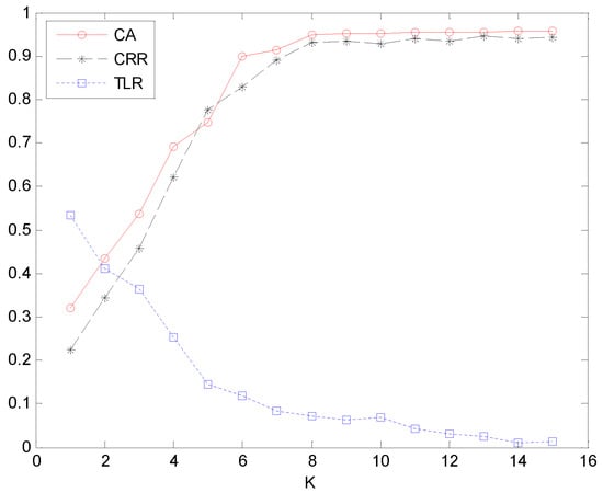
Figure 7.
The CA, CRR and TLR of RPC-EAU based on different K values.
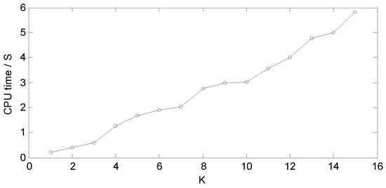
Figure 8.
The CPU time of RPC-EAU based on different K values.
Table 8 showed the values of , and CPU time gradually decrease with the increase in , while increases in contrast. When the value of is 0.1, the RPC-EAU has the best classification performance in this experiment. At this time, the classification accuracy can reach 0.953, the target loss rate can reach 0.013, and the clutter removal rate can reach 0.943. But the corresponding cost is the maximum CPU time, which is 2.98 s. When the value of increases to 0.9, the number of correct identifications for both targets and clutter will decrease, resulting in the values of and only being around 0.82. Of course, the advantage is that it can provide classification results faster, such as a CPU time of only 0.31. The smaller the confidence threshold, the more evidence needs to be corrected in each iteration, resulting in fewer directly output samples. This will inevitably increase the number of iterations for algorithm convergence and CPU time. But the smaller the confidence threshold, the more we need to use sample feature distribution information to correct evidences and optimize the classifier, so as to obtain better recognition results. The experimental results of various evaluation indicators in Table 3 also precisely verify this point.
As shown in Figure 7, the classification accuracy and clutter removal rate of RPC-EAU gradually increase with the increase in K. Especially when k increases from 1 to 8, it can increase from around 0.2 to 0.9. This indicates that limited decision information can lead to misclassification when the number of K-nearest neighbor samples is small. So when K is less than 2, the classification accuracy and clutter removal rate are even less than 0.5. The classification accuracy and filtering rate increase rapidly when K is less than 8, and then no significant changes occur when K is greater than 8, remaining stable at around 0.94. The target loss rate decreases continuously with the increase in K. This indicates that the more K-nearest neighbor evidence used to assist decision-making, the less likely it is to miss target recognition information. This can effectively reduce the misclassification of targets
In Figure 8, it can be intuitively seen that as the value of K increases, the CPU time also keeps increasing. CPU time is less than 0.5 when K is less than 3, reaches around 3 when K is 8, and approaches 6 when K is 16. The values basically exhibit a linear correspondence relationship. Therefore, based on the above indicators, a value of 8 for K is the best choice for this experiment.
4.4. Evidence Update Times
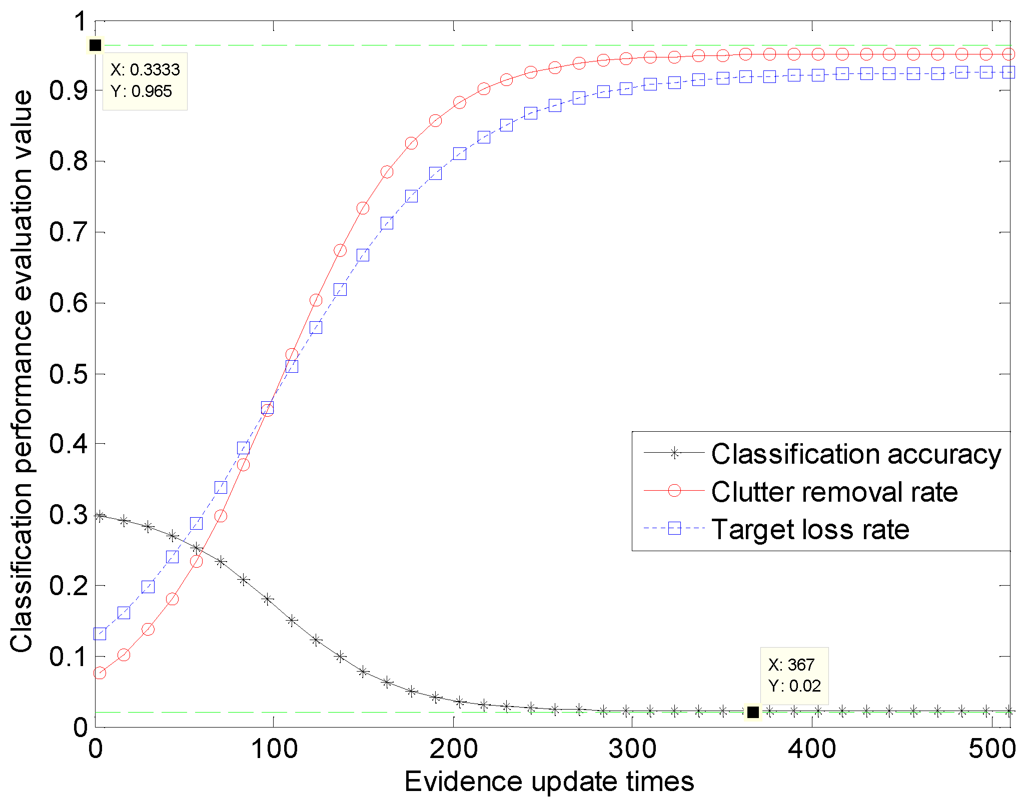
In this section, the relationship between the classification performance and evidence update times of the RPC-EAU is mainly analyzed. And the classification accuracy, target loss rate, clutter removal rate and CPU time are still used as the main indicators for evaluating classification performance. The software environment used in this experiment is also the MATLAB R2023b under the Windows 11 system. The specific relationship curves between the classification performance and the evidence adaptive update times of the RPC-EAU are depicted in Figure 9 and Table 9.
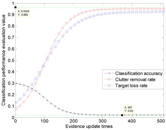
Figure 9.
The specific relationship curves between the classification performance and evidence update times.

Table 9.
The specific relationship between the CPU time and evidence update times.
As show in Figure 9, the classification accuracy and clutter removal rate of RPC-EAU gradually increase with the increase in the evidence update times. Especially when the evidence update times increases from 1 to 300, they can increase from around 0.1 to 0.9. The target loss rate gradually decreases as the evidence update time increases, from the initial 0.3 to around 0.02. It can be seen that once the classification accuracy, clutter removal rate and target loss rate of RPC-EAU reach a certain level, they will not significantly improve with the increase in evidence update times. As shown in Figure 9, the classification accuracy and the clutter removal rate are always below 0.966, while the target loss rate cannot be lower than 0.02. Table 9 indicates that CPU time is generally proportional to the evidence update times. So, when the evidence update times exceed 400 in this experiment, the classification performance no longer significantly improves. Increasing the number of updates at this point will only waste more CPU time.
Therefore, there are some limitations to the performance of the proposed algorithm. Once the classification accuracy, clutter removal rate, and target loss rate of the algorithm reach a certain level, they will not improve again with the increase in the evidence update times. In RPC-EAU, the termination of the evidence adaptive update process is related to the parameters and . And the impact of these two parameters on the performance of RPC-EAU was experimentally analyzed in Section 4.3. It can be seen that the adaptability of RPC-EAU is mainly reflected in the ability to autonomously update the evidence and correct the classifier based on the classification results of each round. This can enhance the learning of the intrinsic characteristics of radar plots. At present, the parameters and of RPC-EAU still need to be manually pre-set according to the experimental scenario. This is also the limitation that restricts the promotion and application of the RPC-EAU.
4.5. Application in Real Traffic Control Radar Data
The real radar plots used in this application instance come from the X-band air traffic control radar. The measurement data include 142 true-value annotation data for three targets under multiple scanning cycles, including 52 shots for target 1, 47 shots for target 2, and 43 shots for target 3. Unlike the synthesized samples in Section 4.1, this radar plot has not been processed by the data processing program and contains a rich variety of clutter plots. The number of clutter plots reaches 1531, which is about 10 times more than the number of targets. This will cause significant interference with accurate classification and pose certain challenges for the performance of each algorithm. Still referring to Section 4.2, the specific parameter settings for each algorithm remain the same.
The numbers of radar plots in each class are shown in Table 10. 30 Monte Carlo experiments were conducted, with half of the radar plot selected for classifier training each time, and the remaining plot used to test the algorithm performance. These indicators include the classification accuracy, target loss rate, clutter removal rate and CPU time. The experiment also recorded the correct and incorrect numbers of target plots obtained by each algorithm during the classification process, represented by and , respectively, as well as the correct and incorrect numbers of clutter, represented by and , respectively. The experimental results for each indicator are shown in Table 11.

Table 10.
The number of radar plots for each class in this application instance.

Table 11.
The experimental results on various indicators.
The statistical results recorded in Table 11 show that the proposed RPC-EAU algorithm performs the best compared to other methods. Although many clutter plots can have a certain impact on classification, RPC-EAU can still maintain a classification accuracy of 0.95. In contrast, the classification accuracy and clutter removal rate of PSO-SVM and IKNN remain around 0.85, with a target loss rate of 0.1. The performance of RPC-FNN and RPC-RNN has improved, with a classification accuracy of around 0.9 for both targets and clutters, and the target loss rate is also less than 0.7. The classification accuracy of RPREC can continue to improve by 4 percentage points, but it takes too much time to reach 33.79 s. RPC-EAU has the highest classification accuracy for targets and clutter, also the lowest target loss rate.
At present, the relative disadvantage of RPC-EAU is that the CPU time cannot be as short as PSO-SVM. The reason is that the classification accuracy and computational time are usually mutual restrained, which means that when pursuing high radar plot classification accuracy, paying a certain cost of computational time is inevitable. Fortunately, the CPU time of RPC-EAU can be maintained at the same level as that of RPC-FNN and RPC-RNN, rather than being as huge as RPREC. This is crucial and meaningful in specific applications.
5. Conclusions
In this study, a radar plot classification algorithm based on evidence adaptive updating called RPC-EAU is proposed. It first constructs ten dimensional features of radar plots for classification. Then, the construction and combination of mass functions based on feature samples distribution are designed. Finally, the design and iterative update strategy of the confidence network classifier are presented. Several experiments based on synthetic and real radar plots are given at the end of the paper. The statistical results from these experiments show that compared with some classic radar plot recognition algorithms, the proposed RPC-EAU algorithm can improve the classification accuracy by 1 to 10 percentage points, reaching around 0.95. The target loss rate of RPC-EAU is also the lowest, around 0.02. The CPU time of RPC-EAU is about 2 to 4 s, which can maintain the same level as RPC-FNN and RPC-RNN. Therefore, RPC-EAU performs the best in the comprehensive evaluation of all indicators.
In addition, RPC-EAU fully utilizes the collaborative decision-making strategy based on classifier and data distribution, which quickly outputs mutually assured results and comprehensively optimizes uncertain data. This not only improves classification accuracy, but also reduces the number of iterations to achieve low computational time. Therefore, it has significant advantages in the classification of uncertain data and has little dependence on samples. However, the evidence adaptive updating and classifier optimization in RPC-EAU rely on the parameters such as confidence thresholds and the number of decision evidences. The correct setting of these parameters for different application scenarios is a challenge. In the future, how to reasonably set algorithm parameters to obtain good results will be a very interesting research topic.
Author Contributions
Writing—original draft preparation, R.Y.; writing—review and editing, Y.Z.; data curation, R.Y.; validation, R.Y. and Y.Z. All authors have read and agreed to the published version of the manuscript.
Funding
This research was funded in part by the National Natural Science Foundation of China, grant number 61804120, and in part by the Natural Science Basic Research Program of Shaanxi, grant number 2021JQ-515.
Institutional Review Board Statement
Not applicable.
Informed Consent Statement
Not applicable.
Data Availability Statement
The processed data required to reproduce these findings cannot be shared, as the data also form part of an ongoing study.
Acknowledgments
The authors are grateful to the reviewers for all their remarks that helped us to clarify and improve the quality of this paper.
Conflicts of Interest
The authors declare no conflicts of interest.
References
- He, Y.; Xiu, J.J.; Liu, Y. Radar Data Processing with Applications, 4th ed.; Electronic Industry Press: Beijing, China, 2022. [Google Scholar]
- Luo, X.W.; Zhang, B.Y.; Liu, J. Researches on the Method of Clutter Suppression in Radar Data Processing. Syst. Eng. Electron. 2016, 38, 37–44. [Google Scholar]
- Duan, C.D.; Han, C.L.; Yang, Z.W. Inshore ambiguity clutter suppression method aided by clutter classification. J. Xidian Univ. 2021, 48, 64–71. [Google Scholar]
- Lin, Q.; Peng, W.; Hu, X.J. Method of Radar Plot True and False Identification Based on Improved KNN. Mod. Radar 2020, 42, 41–45. [Google Scholar]
- Peng, W.; Lin, Q. An Identification Method of True and False Plots Based on PSO-SVM Algorithm. Radar Sci. Technol. 2021, 49, 429–437. [Google Scholar]
- Sun, W.F.; Zhao, L.L.; Ji, Y.G. A false plot identification method based on multi frame clustering for compact HFSWR. Syst. Eng. Electron. 2024, 46, 419–427. [Google Scholar]
- Ma, Y.Z. A Track Screening Algorithm Based on Support Vector Machine. Acoust. Electron. Eng. 2022, 146, 10–13, 18. [Google Scholar]
- Zhang, Y.; Zhang, X.D. True and False Identification Method for Radar Plot Based on Neural Network. Shipboard Electron. Countermeas. 2023, 46, 80–83. [Google Scholar]
- Qi, Y.; Yu, C.; Dai, X. Research on Radar Plot Classification Based on Fully Connected Neural Network. In Proceedings of the 2019 3rd Interna-tional Conference on Electronic Information Technology and Computer Engineering, Xiamen, China, 18–20 October 2019; pp. 698–703. [Google Scholar]
- Liu, Z.; Qi, Y.; Dai, X. Radar Plot Classification Based on Machine Learning. In Proceedings of the 2021 5th International Conference on Electronic Information Technology and Computer Engineering, Tianjin, China, 29–31 October 2021; pp. 537–541. [Google Scholar]
- Wang, H.; Dou, X.H.; Tian, K.Y. Radar Track Classification Method Based on CNN. Shipboard Electron. Countermeas. 2023, 46, 70–74. [Google Scholar]
- Qi, Y.M.; Liu, Z.C.; Yu, C.Z. Research into The Classification Techniques of Radar Plots Based on CNN. Shipboard Electron. Countermeas. 2021, 44, 53–57, 82. [Google Scholar]
- Liu, Z.; Qi, Y.; Dai, X. Radar Plot Classification Method Based on Recurrent Neural Network. In Proceedings of the 2020 4th International Conference on Electronic Information Technology and Computer Engineering, Dali, China, 17–19 July 2020; pp. 611–615. [Google Scholar]
- Peng, W.; Lin, Q. Research on plot authenticity identification method based on PSO-MLP. J. Phys. Conf. Ser. 2020, 1486, 042003. [Google Scholar] [CrossRef]
- Peng, W.; Lin, Q. Research into Plot True and False Identification Method Based on PSO-MLP. Shipboard Electron. Countermeas. 2020, 43, 80–85. [Google Scholar]
- Zhu, X.C.; Zhou, L.; Zhang, Y.T. Plot filter algorithm based on PF-Net. Radar ECM 2022, 42, 19–22, 38. [Google Scholar]
- Meng, W.H.; Lin, Q. The Identification Method of True and False Plots Based on PSO-PNN Algorithm. Comput. Simul. 2022, 39, 11–15. [Google Scholar]
- Dempster, A.P. Upper and lower probabilities induced by a multi-valued mapping. Ann. Math. Stat. 1967, 38, 325–339. [Google Scholar] [CrossRef]
- Shafer, G. A Mathematical Theory of Evidence; Princeton University Press: Princeton, NJ, USA, 1976. [Google Scholar]
- Denoeux, T. 40 years of Dempster-Shafer theory. Int. J. Approx. Reason. 2016, 79, 1–6. [Google Scholar] [CrossRef]
- Denoeux, T. A k-nearest neighbor classification rule based on Dempster-Shafer theory. IEEE Trans. Syst. Man Cybern. 1995, 25, 804–813. [Google Scholar] [CrossRef]
- Ma, Z.F.; Tian, H.P.; Liu, Z.C.; Zhang, Z.W. A new incomplete pattern belief classification method with multiple estimations based on KNN. Appl. Soft. Comput. 2020, 90, 106175. [Google Scholar] [CrossRef]
- Meng, J. Research and Application of Data Classification Based on the Theory of Belief Functions; University of Science and Technology Beijing: Beijing, China, 2021. [Google Scholar]
- Liu, Z.G.; Qiu, G.H.; Mercier, G.; Pan, Q. A transfer classification method for heterogeneous data based on evidence theory. IEEE Trans. Syst. Man Cybern. Syst. 2021, 51, 5129–5141. [Google Scholar] [CrossRef]
- Liu, S.T.; Li, X.J.; Zhou, Z.J. Review on the application of evidence theory in patten classification. J. CAEIT 2022, 17, 247–258. [Google Scholar]
- Zhang, Z.; Tian, H.; Yan, L.; Martin, A.; Zhou, K. Learning a creedal classifier with optimized and adaptive multiestimation for missing data imputation. IEEE Trans. Syst. Man Cybern. Syst. 2022, 52, 4092–4104. [Google Scholar] [CrossRef]
- Liu, Z.G.; Pan, Q.; Dezert, J.; Mercier, G. Credal c-means clustering method based on belief functions. Knowl.-Based Syst. 2015, 74, 119–132. [Google Scholar] [CrossRef]
- Denoeux, T.; Sriboonchitta, S.; Kanjanatarakul, O. Evidential clustering of large dissimilarity data. Knowl.-Based Syst. 2016, 106, 179–195. [Google Scholar] [CrossRef]
- Denoeux, T.; Kanjanatarakul, O. Evidential clustering: A review. In Proceedings of the 5th International Symposium on Integrated Uncertainty in Knowledge Modelling and Decision Making, Da Nang, Vietnam, 30 November–2 December 2016; pp. 24–35. [Google Scholar]
- Zhang, Z.; Liu, Z.; Martin, A.; Zhou, K. Dynamic evidential clustering algorithm. Knowl.-Based Syst. 2021, 213, 106643. [Google Scholar] [CrossRef]
- Denoeux, T. NN-EVCLUS: Neural network-based evidential clustering. Inf. Sci. 2021, 572, 297–330. [Google Scholar] [CrossRef]
- Jiao, L.; Denoeux, T.; Liu, Z.-G.; Pan, Q. EGMM: An evidential version of the gaussian mixture model for clustering. Appl. Soft Comput. 2022, 129, 109619. [Google Scholar] [CrossRef]
- Xie, B.L. Research on Muli-Sensor Data Fusion Method Based on DS Evidence Theory; Henan University: Kaifeng, China, 2022. [Google Scholar]
- Denoeux, T. Decision-Making with Belief Functions: A Review. Int. J. Approx. Reason. 2019, 109, 87–110. [Google Scholar] [CrossRef]
- Liu, Z.G.; Zhang, X.; Niu, J.; Dezert, J. Combination of Classifiers With Different Frames of Discernment Based on Belief Functions. IEEE Trans. Fuzzy Syst. 2021, 29, 1764–1774. [Google Scholar] [CrossRef]
- Lian, C.; Ruan, S.; Denoeux, T.; Li, H.; Vera, P. Spatial evidential clustering with adaptive distance metric for tumor segmentation in FDGPET images. IEEE Trans. Biomed. Eng. 2017, 65, 21–30. [Google Scholar] [CrossRef]
- Lian, C.; Ruan, S.; Denoeux, T.; Li, H.; Vera, P. Joint tumor segmentation in PET-CT images using co-clustering and fusion based on belief functions. IEEE Trans. Image Process. 2018, 28, 755–766. [Google Scholar] [CrossRef] [PubMed]
- Liu, S.; Guo, X.J.; Zhang, L.Y. FMEA evaluation of all-electric ship propulsion Based on fuzzy confidence theory. Control Eng. China 2021, 28, 1807–1813. [Google Scholar]
- Han, X.X.; Wang, J.; Chen, Y. Safety assessment of water supply and drainage based on evidential reasoning rule. Sci. Technol. Eng. 2021, 21, 13758–13764. [Google Scholar]
- He, K.X.; Wang, T.; Su, Z.Y. Improved abnormal condition detection based on evidence K-nearest neighbor and its Application. Control Eng. China 2022, 29, 655–660. [Google Scholar]
- Abdelkhalek, R.; Boukhris, I.; Elouedi, Z. An evidential collaborative filtering approach based on items contents clustering. In Belief Functions: Theory and Applications, Proceedings of the 5th International Conference, BELIEF 2018, Compiègne, France, 17–21 September 2018; Springer International Publishing: Berlin/Heidelberg, Germany; pp. 1–9.
- Abdelkhalek, R.; Boukhris, I.; Elouedi, Z. An evidential clustering for collaborative filtering based on users preferences. In Modeling Decisions for Artificial Intelligence, Proceedings of the 16th International Conference, MDAI 2019, Milan, Italy, 4–6 September 2019; Springer International Publishing: Berlin/Heidelberg, Germany, 2019; pp. 224–235. [Google Scholar]
- Yang, R.; Zhao, Y.B.; Shi, Y. RPREC: A Radar Plot Recognition Algorithm Based on Adaptive Evidence Classification. Appl. Sci. 2023, 13, 12511. [Google Scholar] [CrossRef]
- Yang, R.; Zhao, Y.; Yang, T. A recognition algorithm of radar plots based on confidence function and self-updating classifier. Sci. Technol. Eng. 2023, 23, 8236–8242. [Google Scholar]
Disclaimer/Publisher’s Note: The statements, opinions and data contained in all publications are solely those of the individual author(s) and contributor(s) and not of MDPI and/or the editor(s). MDPI and/or the editor(s) disclaim responsibility for any injury to people or property resulting from any ideas, methods, instructions or products referred to in the content. |
© 2024 by the authors. Licensee MDPI, Basel, Switzerland. This article is an open access article distributed under the terms and conditions of the Creative Commons Attribution (CC BY) license (https://creativecommons.org/licenses/by/4.0/).


