Research on the Characteristic State of Rockfill Materials and the Evolution Mechanism at the Microscopic Scale

Abstract

In this study, the real particle morphology of rockfill materials is obtained through three-dimensional scanning technology, and flexible boundary conditions are established by coupling the discrete element method and the finite element method. Then, a large-scale three-axis numerical simulation test is carried out on the rockfill materials to study the macroscopic mechanical properties and the change rule of the microscopic view of the rockfill materials in different characteristic states. The macroscopic results show that the stress–strain curves of the rockfill materials can be divided into softening and hardening curves. The phase transition, peak, and critical states of the softening-type curves show different mechanical properties, but no clear distinction between the characteristic state changes can be seen in the hardening-type curves. The microscopic results show that the displacement of the upper and lower parts of the flexible boundary of the softening curve increases with loading, and there is no obvious displacement in the middle part, but the middle particles undergo rotational deformation. An “X” shear band appears, and the strength of the force chain and the coordination number tend to increase first and then decrease. The flexible boundary displacements of the hardening-type curves are similar to those of the softening-type curves, but the central particles show a large number of cleavages instead of shear zones, and the force chain strength and coordination number levels show a continuous upward trend.

1. Introduction

For rockfill dams made of rockfill particles, as the dam height increases, there are stricter requirements for slope stability, deformation control, and seismic safety [1,2]. To address these requirements, the peak stress ratio and shear expansion–stress ratio are used to establish functional relationships within an intrinsic structure model [3], which is a significant step in optimizing the intrinsic constitutive relationship.

The phase change, peak, and critical states are three significant characteristic states of rock particles. The phase change state was initially proposed to represent the state of sandy soil, where the pore water pressure decreases or the deviatoric stress increases under undrained shear stress [4], signifying the densest state. This is crucial in constructing an elastic–plastic intrinsic model [5,6]. The concept of a characteristic state is further extended to describe the stress level at the transition from volume compression to volume expansion in sandy soils under drainage conditions, which is the turning point from body contraction to body expansion [7]. The peak state is relatively well understood, representing the condition corresponding to the maximum stress or stress ratio value in the soil during loading [8]. The critical state is the limit achieved during soil deformation when the effective mean positive stress, shear stress, and volume cease to change [9], and it serves as a stable reference state for analysis.

Researchers have analyzed and studied the three characteristic states of rockfill materials through physical tests and numerical simulations. Large-scale indoor triaxial tests are the most commonly used physical tests. Yang G et al. [10] carried out a series of large-scale triaxial tests on rockfill materials with different maximum grain sizes to investigate the effect of grain size distribution on the critical state of rockfill materials. They found that the intercept and gradient of the critical state line along the plane decreased as the gradient became wider with increasing grain size, while the gradient of the critical state line along the plane increased with increasing grain size. Ning F et al. [11] investigated the effect of stress paths on the evolution of the critical state and the particle crushing gradation of rockfill materials using large-scale triaxial compression tests. The average effective stress p′, deviatoric stress q, and pore ratio e along different stress paths reached the same critical state line (CSL). Differences in the small and medium principal stress ratios in a true triaxial compression test also have a greater effect on the mechanical properties of the rockfill materials [8]. The medium principal stress ratio has a greater effect on the critical state friction angle, peak state friction angle, and maximum shear expansion of the simulated rockfill materials. Xiao Y et al. [12] conducted a series of large-scale triaxial compression tests on a Tacheng Rock Mound (TRM). They found that its deformation behavior was affected by density and stress and that the critical state friction angle of the TRM decreased with increasing initial confining pressure. The integration of histogram anisotropy into the description of critical state damage revealed that the orientation of the histogram tensor is isotropic concerning the stresses in the critical state [13]; this technique provides a unique value related to the shear mode or Lode angle. Cheng J et al. [14] investigated the mechanical properties of rockfill materials with different wetting–drying cycles and wetting durations and found that deterioration occurred in the form of a decrease in yield stress and an increase in compressibility, which varied nonlinearly with the number of wetting–drying cycles and wetting duration.

The critical state of a rockfill material is significantly influenced by its density, grade, and confining pressure. Strain softening is most evident under a low confining pressure and high density, while strain hardening is observed under the opposite conditions [15,16,17,18]. As rockfill materials’ deformation and strength properties are heavily influenced by their microscopic structure, a detailed study of rockfill materials at this level can effectively explain their macroscopic mechanical phenomena. Scholars have used the discrete element method for numerical simulations to conduct triaxial numerical simulation tests on rockfill materials. This method was first proposed by Cundall [19] to study the macroscopic behavior of granular materials at the microscopic scale in rock mechanics.

Subsequently, some scholars have extensively analyzed rockfill materials at the microscopic scale using various parameters (Han H, Zhou W, etc. [20,21]) to study the effect of particle shape on the mechanical properties of rockfill materials through the establishment of different shapes of rockfill material particles in three-axis numerical simulation tests and found that the more complex the shapes of the particles are, the closer the simulation is to the mechanical properties of real rocks. The mechanical properties of rockfill materials are not only affected by microscopic factors, such as particle morphology and grading, but also closely related to different loading stress paths. Zhang R, Xu M et al. [22,23] investigated the macro- and micromechanical properties of rockfill materials under different stress paths, and the results showed that there was a significant difference in the effect of stress paths on the deviatoric stress–strain, and strain–volume change characteristics of rockfill materials. The three-dimensional (3D) discrete element method (DEM) for triaxial tests has been used to simulate and study the shear behavior of granular materials [24]. DEM simulations of triaxial tests under membrane boundary conditions consisting of membrane particles were carried out, and the DEM model under the membrane boundary conditions suitably reflected the evolution of the sample’s irregular deformations and the shear bands during the shear process. This study greatly improves the accuracy of the DEM simulations of triaxial tests under membrane boundary conditions. A new algorithm was proposed to reproduce flexible film boundaries in triaxial tests [25]. A comparison of triaxial tests with flexible and rigid boundaries was made at the macroscopic scale and the microscopic scale, and it was found that flexible film boundaries better reflect physical test variations. A triaxial test based on the discrete element method (DEM) found that the contact force chains in the microscopic structure can reflect their corresponding macroscopic behavior, and the greater the number of force chains is, the greater the peak strength [26]. DEM simulations under real triaxial conditions were also carried out to investigate the critical state and swelling properties of granular materials at both the macroscopic and microscopic levels [27], and it was found that both the contact direction and the contact force affect the mechanical properties of granular materials. Cai G, Qin Y et al. [28,29] investigated granular materials by discrete element numerical simulation and analyzed the deformation and damage process of a numerical model using a deviatoric stress-strain curve, microcracks, displacement fields, stress fields, and energy fields. It was found that the displacement field can more significantly show the shear damage region and form, and displacement zoning appears.

Therefore, in this paper, based on a triaxial test of rockfill materials, a numerical simulation is used to carry out a large-scale triaxial numerical simulation test under different densities. Macroscopically, the changes in the phase transition, peak, and critical states of rockfill materials are studied, and microscopically, the deformation and damage mechanism of rockfill materials are revealed from the aspects of the shear band, flexible membrane displacement, contact force chain, coordination number, etc., to provide a reference from a detailed perspective for the analysis of changes in the characteristic states of rockfill materials.

2. Numerical Model Construction

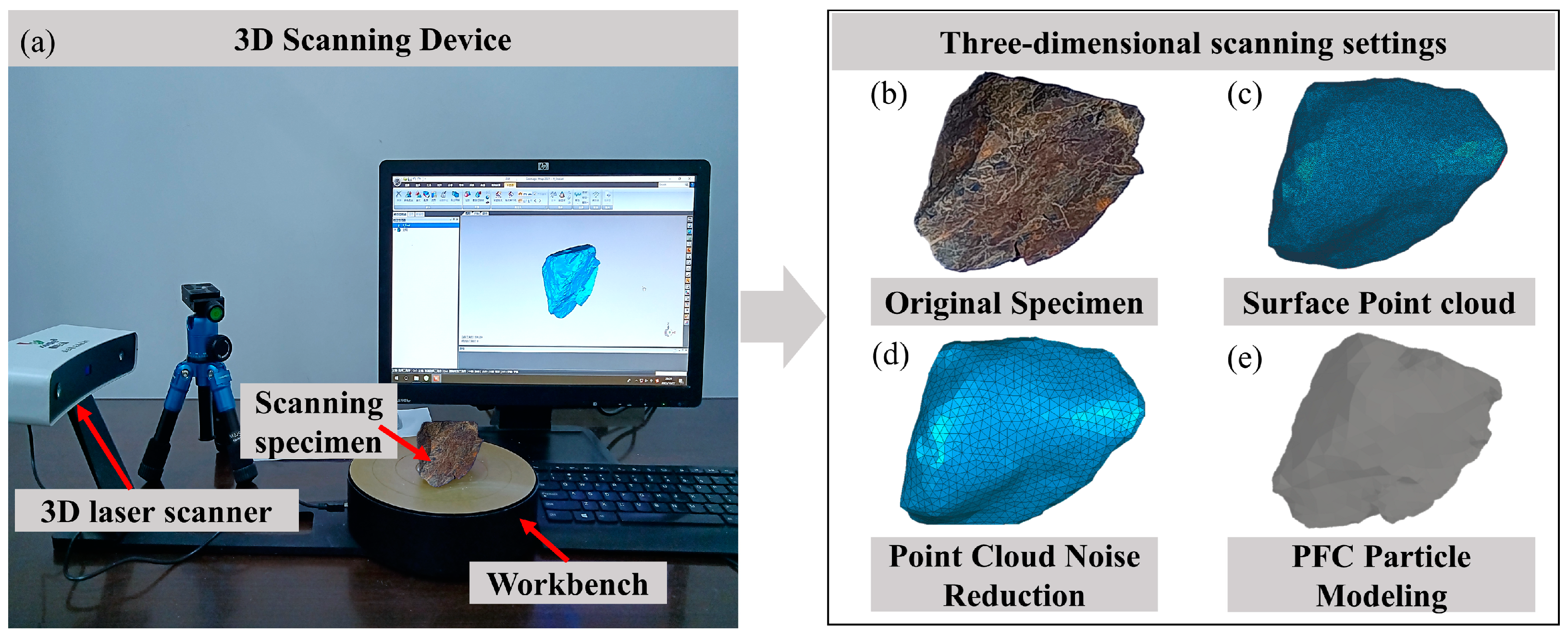
2.1. Three-Dimensional Shape Recognition of Rockfill Materials

The appearance, grading, densification, shape, and size of stacked stone particles control rockfill materials’ strength and deformation characteristics. In this section, the 3D laser scanning data of the block stone particles of the rockfill material are used to analyze the particles’ shape characteristics and establish 3D microscopic characterization and reconstruction methods for the particles.

Blue light scanning technology, recognized for its advanced, fully automatic, and high-precision) three-dimensional scanning capabilities, is used for this purpose [30]. The SENSE-DS2+ (KANGKE 3D) (Guangzhou Concord Information Technology Co., Guangzhou, China) blue light scanner is equipped with a light emitting diode (LED) cold light source with a wavelength of 450 mm or less, strong anti-interference, high brightness, low power consumption, and fast response, with an accuracy of 0.05 mm. The scanned block shape is more ideal. The stacked stone specimen is placed on an automatic rotating table during scanning, and the surface point cloud data of the granular specimen are acquired by scanning, as illustrated in Figure 1a. The particle surface point cloud in Figure 1c comprises nearly one million data points directly used for discrete element modeling. This approach poses challenges in locating contact points between particles due to the high data density. To address this, the particle surface point cloud data are imported into the three-dimensional reverse engineering software Geomagic Wrap (2021) to reduce the data noise, creating a smooth triangular surface piece to obtain a smooth closed surface that approximates the real geometric boundary of the particle specimen (Figure 1d). Finally, the closed surface is imported into the discrete element software PFC3D (6.0) through a self-programmed program, as shown in Figure 1e. This comprehensive process enables detailed analysis and modeling of the shape characteristics of stacked stone particles to understand their mechanical properties further.

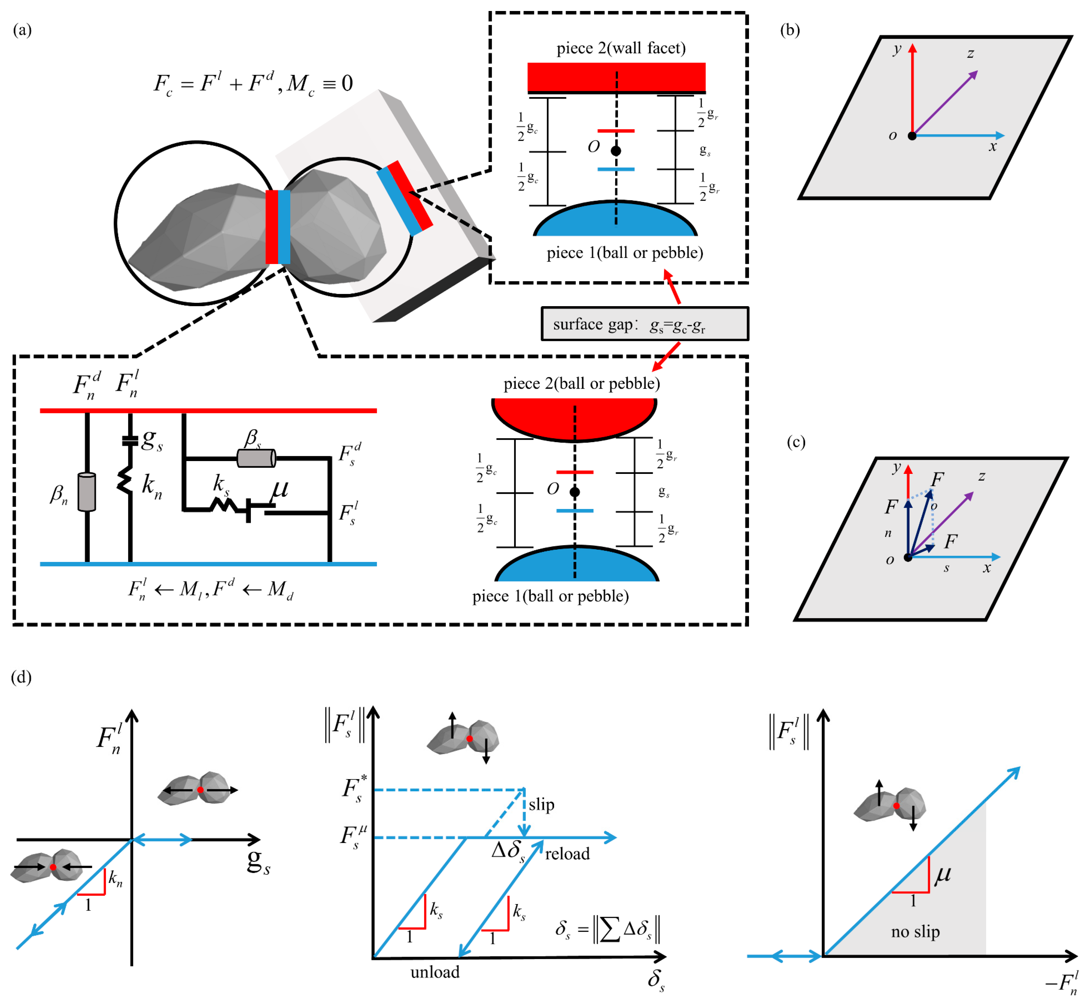
2.2. Rigid Block Contact Modeling in Particle Flow Algorithms

The discrete element software PFC (6.0) effectively captures rockfill materials’ mechanical properties and considers their particle shape effect [31]. During the construction of numerical specimens, the contact state between particles of the ball unit is easy to determine with high computational efficiency due to its simple shape. However, the closure between spherical particles is weak, which contradicts the physical properties of rockfill materials [32]. Although clump units can realistically simulate rockfill material particles, they require more computer memory and computation time [33]. The rblock unit maintains the realism of the clump unit. The computational efficiency is significantly improved by having only one contact between the rblock unit and other units, as determined by the outer circle [34].

In the discrete element method, the contact model serves as a mechanical criterion for the interaction between particles, determining the macroscopic and microscopic mechanical properties of the entire particle system. The rblock unit can interact with the ball, clump, and wall regions in 3D, employing a linear contact model that defines the behavior of an infinitesimal interface. This model decomposes the contact force into linear and damped components, where M_c ≡ 0 and F_c = F_l + F_d. The choice of the linear contact model is motivated by its suitability for meeting the contact requirements between the blocks and improving computational efficiency. The elements of the linear contact model consist of normal and tangential springs with stiffnesses k_n and k_s, respectively; sliding elements with friction factors μ; normal and tangential dampers with damping coefficients β_n and β_s; and pressure-bearing elements identifying the amount of interparticle overlap g_s, as shown in Figure 2a. When the reference gap is zero, the hypothetical surface [35] coincides with the surface of the workpiece, and the relative displacement increment at the contact during the time step (Δt) is calculated from Δδ_n and Δδ_s in Equation (1):

$$\begin{array}{c}\Delta {\delta }_{\mathrm{n}}:=\alpha \Delta {\delta }_{\mathrm{n}},\Delta {\delta }_{\mathrm{s}}:=\alpha \Delta {\delta }_{\mathrm{s}}\\ \mathrm{with} \alpha =\{\begin{array}{c}\frac{g_s}{g_s-{(g_s)}_0},{(g_s)}_0>0{ \mathrm{and} \mathrm{g}}_s>0\\ 1, \mathrm{otherwise} \end{array}\end{array}$$

(1)

where g_s is the surface gap and (g_s)₀ is the surface gap at the beginning of the time step.

A local Cartesian coordinate system (x, y, z) is established at the contact point O, where y is parallel to the contact normal, and x and z are mutually perpendicular following the right-hand rule with y, as illustrated in Figure 2b. In this coordinate system, the contact force F_c in the linear contact model can be decomposed into the normal contact force F_n and the tangential contact force F_s, as shown in Figure 2c. The following formula calculates the contact force F_c.

$$F_c=F_n+F_s$$

(2)

Among them:

$$\{\begin{array}{c}{F}_n=F_n^l+F_n^d\\ F_s=F_s^l+F_s^d\\ F^l=F_n^l+F_s^l\\ F^d=F_n^d+F_s^d\end{array}$$

(3)

where $F^l$ is the linear contact force, decomposed into a normal force $F_n^l$ and a tangential force $F_s^l$; $F^d$ is the viscous damping force, decomposed into a normal force $F_n^d$ and a tangential damping force $F_s^d$. As shown in Figure 2d, the normal and tangential components $F_s^l$ of the linear contact force in each calculation cycle are updated in increments as follows:

$$F_n^l=\{\begin{array}{c}{(F_n^l)}_0+k_n\Delta {\delta }_n,g_s\ge 0\\ 0,g_s<0\end{array}$$

(4)

$$F_s^l=\{\begin{array}{c}{F}_s^{*}={(F_s^l)}_0-k_s\Delta {\delta }_s,\Vert F_s^{*}\Vert \le \Vert F_s^{\mu }\Vert \\ F_s^{\mu }=-\mu F_n^l(F_s^{*}/\Vert F_s^{*}\Vert ),\Vert F_s^{*}\Vert >\Vert F_s^{\mu }\Vert \end{array}$$

(5)

where ${(F_n^l)}_0$ and ${(F_s^l)}_0$ are the initial normal and tangential forces in the current calculation cycle; k_n is the normal stiffness; $\Delta {\delta }_n$ and $\Delta {\delta }_s$ are the normal and tangential relative displacements, respectively; $F_s^{*}$ is the tangential force when there is no sliding; and $F_s^{\mu }$ is the tangential force when there is sliding between particles in the current calculation cycle.

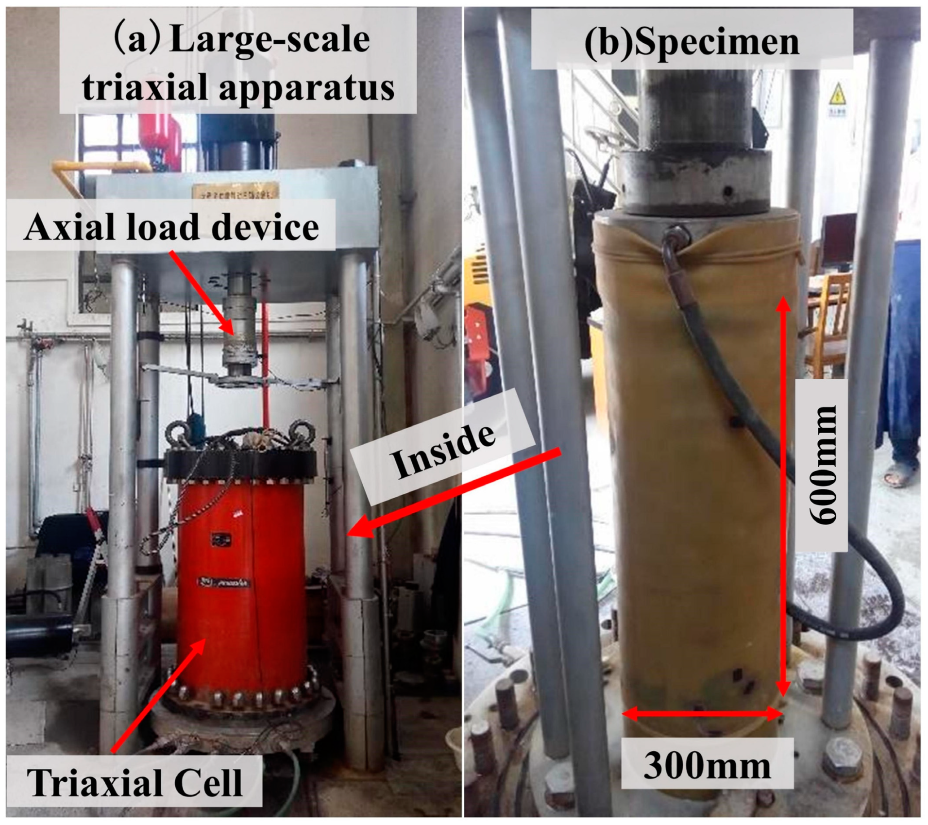
2.3. Discrete Element Triaxial Test Servo Mechanism

In triaxial testing, the specimen maintains a stable state of peri-compression during consolidation and shear. In contrast, it is only possible to specify specific velocities for the wall units, not the force or stress properties in numerical simulation. Consequently, controlling the velocity of the wall becomes the sole method for accurately controlling the force exerted by the wall on the internal particles. The velocity of wall movement can be expressed by Equation (6):

$${\dot{u}}^{(w)}=G({\sigma }^{measured}-{\sigma }^{required})=G\Delta \sigma$$

(6)

where ${\dot{u}}^{(w)}$ is the wall contraction (or expansion) rate; G is the servo parameter; σ^measured is the real-time stress; σ^measured is the target stress; and Δσ is the difference between the real-time and target stresses.

Since the stresses in the wall cannot be detected directly in the software, the stresses can be obtained by measuring the combined external forces on the wall and dividing by the contact area. Equation (7) describes the incremental wall confinement stress Δσ^(ω) caused by the confinement motion in one time step.

$$\Delta {\sigma }^{(w)}=\frac{k_n^{(w)}{N}_c{\dot{u}}^{(w)}\Delta t}{A}$$

(7)

where $k_n^{\left(\omega \right)}$ is the average normal stiffness of the particle-wall contact, N_c is the total number of particles in contact with the wall, ${\dot{u}}^{(w)}\Delta t$ is the distance traveled by the loaded wall in one time step, and A is the wall area.

The absolute value of the increase in the confining stress caused by wall contraction or expansion was less than the difference between the measured and desired stress to maintain stability. This ensures less change in the confining pressure due to wall movement in each step of the calculation, which is specified as follows:

$$\left|\Delta {\sigma }^{(w)}\right|=\left|\frac{k_n^{(w)}{N}_c{\dot{u}}^{(w)}\Delta t}{A}\right|<\alpha \left|\Delta \sigma \right|$$

(8)

where α is the relaxation factor.

Taking G > 0 and Δσ > 0, the servo tuning factor can be obtained as:

$$G=\frac{\alpha A}{k_n^{(w)}{N}_c\Delta t}$$

(9)

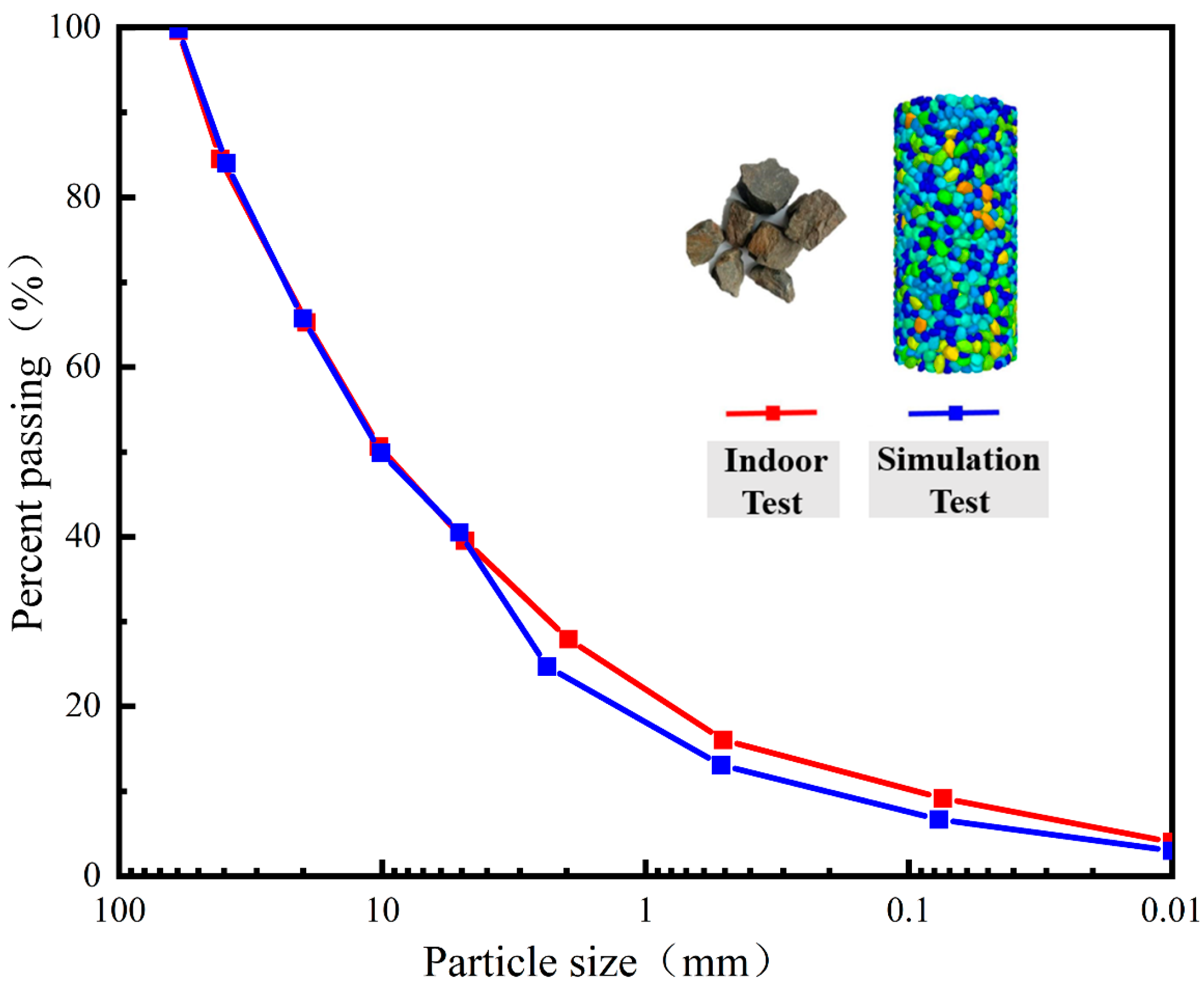
2.4. Specimen Generation

The rockfill materials used in the test serve as the main construction material of a water conservancy hub project panel rockfill dam. The lithological units of the material are the middle and lower Carboniferous medium-thick layer of chert and dolomitic chert, which is a medium-hard to hard rock with a measured specific gravity of 2.66 g/cm³ and a dry density of 2.15 g/cm³. The maximum size of the rock lumps is 60 mm. This study uses a large-scale multifunctional static-dynamic triaxial tester with a capacity of 2000 kN, designed for large-scale static-dynamic properties of soil, rockfill, and concrete materials. The testing device consists of a triaxial unit, an axial loading device, a unit pressure control device, a digital servo control unit, and a measurement and data acquisition system. The specimen is 300 mm in diameter and 600 mm in height. The vertical and confining pressure servos can be controlled separately or simultaneously and the axial strain is measured using a displacement transducer mounted on the loading punch. The volumetric strain can be measured by the water that flows into or out of the specimen through the volumetric tube. The stress or strain control can be freely converted during the test, and the entire testing process is computer-controlled with automated data collection and real-time visualization. Figure 3 shows the equipment used for this procedure.

The consistency of the simulated particles is ensured with the actual particle gradation in the chamber. A gradation generation program was developed in the FISH language, which enables the particle gradation of the generated granular flow model of rockfill materials to align with that of the chamber test. Additionally, it allows the generation of model specimens of rockfill materials with any specified gradation as needed. The gradation curves of the simulated particles can then be compared with the test gradation curves, as shown in Figure 4.

In indoor conventional triaxial tests, a specimen is often wrapped in a rubber membrane to study its mechanical properties, and stresses are applied through the top and bottom loading plates. In the numerical simulation test, the wall unit can be used to simulate the force on the specimen, but the wall established by the wall unit is rigid, and the specimen cannot undergo lateral deformation or other phenomena that occur during the loading process. The method of replacing the lateral wall with a ball unit to simulate the flexible rubber membrane has a large number of particles, which is difficult to carry out in the calculation because of the high requirements on the arithmetic power of the equipment and the long duration of the calculation process. The shell unit in FLAC3D (6.0) can simulate the lateral deformation in the numerical test, and the numerical model established through the coupling of PFC (6.0) and FLAC3D (6.0) is faster in the calculation process, so this paper establishes the numerical model by this method, as shown in Figure 5. Figure 5a shows that the specimen size is 300 × 600 mm, and the stacked rock particles are simulated by the rblock unit because the shape of the stacked rock particles has been obtained by 3D scanning technology and imported into the model. The contact between the stacked rock particles can be simulated directly by the linear model. The contact model between the loading plate and the gravel particles, between the particles and between the particles and the flexible membrane is set as a linear contact model.

As shown in Figure 5b, the specimen volume consists of three parts: Part I is a cone composed of the center point O and the wall at the lower edge of the upper wall; Part II is a cone composed of the center point O and the wall at the upper edge of the lower wall; and Part III is a tetrahedron composed of the center point O and the nodes on the shell unit, which is shown by the enlarged schematic diagram of Figure 5b. The bottom of the tetrahedron is a triangle formed by the nodes on the shell unit, which forms a tetrahedron with the center point O of the specimen [24]. The volume of a cone can be calculated directly via the following formula. In the tetrahedron volume calculation, the coordinates of the four vertices are set to O(x₀, y₀, z₀), M(x₁, y₁, z₁), N(x₂, y₂, z₂), and R(x₃, y₃, z₃), and the coordinates of the tetrahedron centroid, point O, can be expressed as:

$$O(x_0,y_0,z_0)\{\begin{array}{c}{x}_0=\frac{x_1+x_2+x_3}{3}\\ y_0=\frac{y_1+y_2+y_3}{3}\\ z_0=\frac{z_1+z_2+z_3}{3}\end{array}$$

(10)

The area of the base S_A in tetrahedron V_i is calculated using the following equation:

$$\overrightarrow{m}=(x_1-x_0,y_1-y_0,z_1-z_0)$$

(11)

$$\underset{\_}{n}=(x_2-x_0,y_2-y_0,z_2-z_0)$$

(12)

$$S_A=\frac{1}{2}|\overrightarrow{m}\times \overrightarrow{n}|$$

(13)

The stress applied to tetrahedron V_i can be expressed as:

$${\displaystyle \sum \sigma ={\sigma }_3\times {\displaystyle \sum S_A}}$$

(14)

where σ₃ is the confining pressure and ${\displaystyle \sum S_A}$ is the total area of the boundary surface of the shell membrane.

The specimen volume was calculated by the following formula:

$$V=V_1+V_2+{\displaystyle \sum _1^n{V}_i}=\frac{1}{3}\pi r^{2}h+{\displaystyle \sum _1^n{V}_i}, i=1,2,3,\cdots ,n$$

(15)

wherein

$$V_i=\frac{1}{6}\left|\begin{array}{c}{x}_1^i-x_0 y_1^i-y_0 z_1^i-z_0\\ x_2^i-x_0 y_2^i-y_0 z_2^i-z_0\\ x_3^i-x_0 y_3^i-y_0 z_3^i-z_0\end{array}\right|=\frac{1}{6}\left|\begin{array}{c}{x}_0 y_0 z_0 1\\ x_1^i y_1^i z_1^i 1\\ x_2^i y_2^i z_2^i 1\\ x_3^i y_3^i z_3^i 1\end{array}\right|$$

(16)

where n is the number of shell unit wall triangles.

2.5. Microscopic Parameter Calibration

In the numerical simulation, the values of the fine-scale parameters are key to the simulation results. First, considering the contact friction and lack of cementation between the rockfill particles, a linear contact model is used to describe the mechanical properties of the rockfill materials. Second, to better describe and respond to the mechanical properties of the rockfill materials, the model parameters E, k_n, k_s and μ [36], which have a greater influence on them, are selected. A blind adjustment of the microscopic parameters during the calibration process will increase the difficulty of the test to a large extent. This paper quickly determines the range of parameter values on the basis of mastering the intrinsic connection between the microscopic parameters and macroscopic indices (e.g., the effective modulus E has the highest degree of influence on the elastic modulus, k_n and k_s have a significant influence on the Poisson’s ratio ν, and the coefficient of friction μ mainly affects the peak strength [37]). Finally, minor parameter fine-tuning was carried out according to the indoor test results until the simulation results were in good agreement with the indoor results, and the following microscopic parameters were finally determined, as shown in

Table 1. Parameter setting for the particle flow numerical simulation.

Materials	E/Pa	kn/(N·m–1)	ks/(N·m–1)	μ	ν	Film Thickness/(mm)
Particles	55 × 109	7.85 × 108	6.28 × 108	0.6
Boundary	7.86 × 106	—	—	0	0.47	5

.

The parameters outlined in Table 1 were used for large-scale triaxial numerical simulations, and a relative comparison of the numerical test simulations and the indoor triaxial test results is shown in Figure 6. The simulation results of the bias stress-axial strain relationship of the numerical simulation test) agree well with the indoor test results, and the stress(strain curve) evolution trend is basically the same. This alignment indicates that the microscopic-scale parameters calibrated in this study can effectively capture the deviatoric stress-axial strain relationship of the rockfill materials. The purpose of this paper is to study the deformation characteristics and variations in the characteristic state parameters of rockfill materials. Therefore, large-scale triaxial numerical simulation tests were conducted at three densities of 0.30, 0.60, and 0.90, corresponding to initial pore ratios of 0.368, 0.336, and 0.215, respectively, under confining pressures of 300, 600, and 900 kPa.

3. Test Results and Analysis

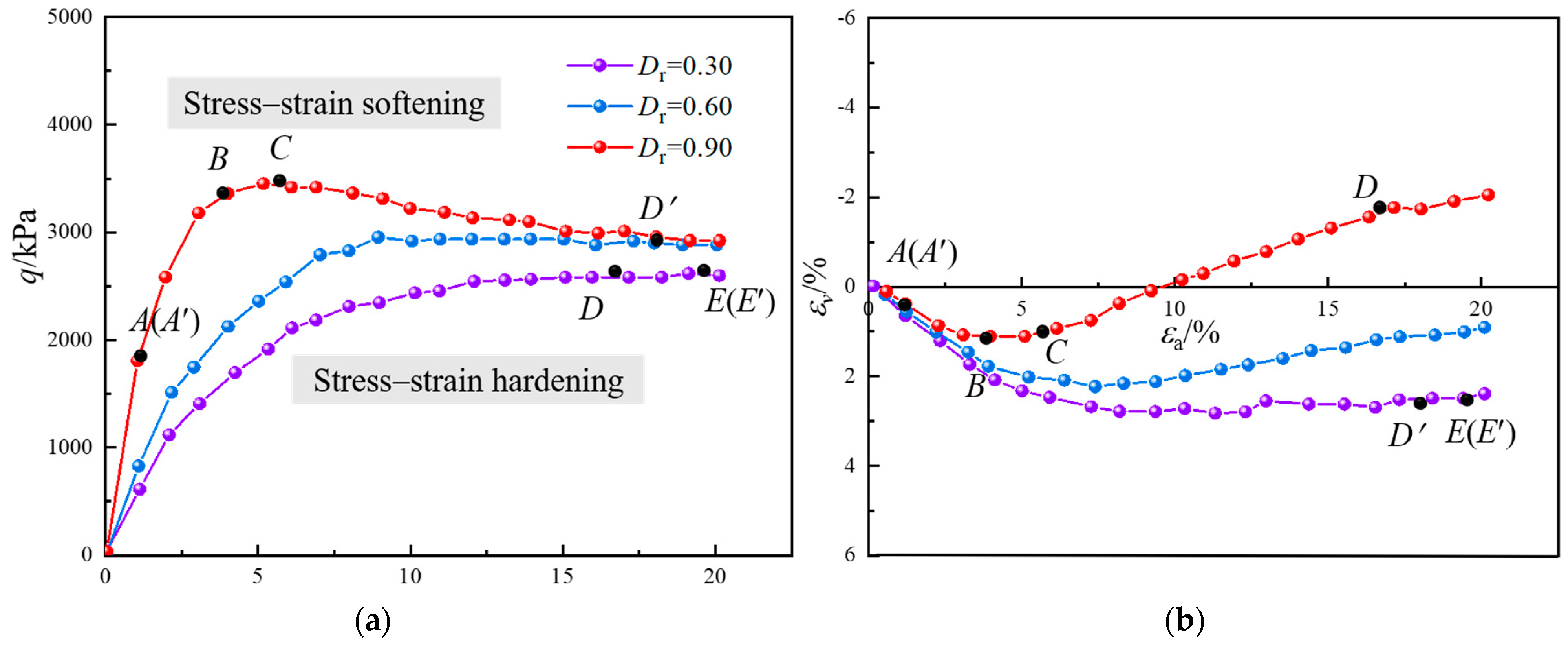
3.1. Deformation Characteristics of Rockfill Materials Considering the Effect of Density

The deviatoric stress and volumetric strain versus axial strain curves for specimens with a relative compaction of D_r = 0.60 under different confining pressures are shown in Figure 7. Five points, A, B, C, D, and E, divide the loading process into five stages. Point A represents the initial yield with the beginning of the volume change; point B represents the phase change state with the beginning of the volumetric strain shift from shear contraction to shear expansion; point C represents the peak strength, indicating maximum volume compression (stress-strain hardening) or the fastest volume expansion (stress-strain softening) when the rockfill materials reach the limit of resistance to external forces; point D represents the critical state with gradual volume change tending to level off; and point E represents the end point of loading. When the confining pressure is low (σ₃ = 300 kPa), the stress-strain relationship exhibits strain softening, as illustrated in Figure 7. As the axial strain increases, the deviatoric stress increases, with body shrinkage deformation due to the volumetric strain. When the axial strain is loaded to approximately 4%, the volumetric strain compression reaches the limit and transforms into volume expansion. At this point, the specimen is in the phase change state (point B). The specimen enters the damage state when the deviatoric stress reaches the peak (point C), and the body expansion deformation becomes more distinct. Furthermore, as the shear proceeds, the deviatoric stress starts to decrease and stabilize, along with the stabilization of the volumetric strain, which ultimately results in the critical state (point D). When the confining pressure is high (σ₃ = 900 kPa), the stress-strain relationship shows strain hardening and the deviatoric stress increases with increasing axial strain, resulting in the corresponding shrinkage of the specimen’s corresponding volume. The volumetric strain shows body shrinkage deformation, which continues until the end of loading. The deviatoric stress does not exhibit a peak during the loading process. At this point, the specimens’ phase change, peak, and critical states occur in the same state (D′). The confining pressure determines the deformation characteristics of specimens with distinct densities. The lower the confining pressure, the more distinct the strain softening phenomenon; the higher the confining pressure, the more distinct the strain hardening phenomenon.

The deviatoric stress and volumetric strain versus axial strain curves for specimens with different densities at a confining pressure of 600 kPa are shown in Figure 8. When the relative density of the specimen is large (D_r = 0.90), the stress-strain relationship exhibits a strain-softening relationship. As loading proceeds, the deviatoric stress increases initially, with body shrinkage resulting from volumetric strain. A loading of axial strain up to approximately 2% results in the phase change state of the specimen (point B) and the maximum compression value of the volumetric strain, which subsequently results in volume expansion. This is followed by a more noticeable body expansion deformation, resulting in the fastest volume expansion when the axial strain reaches approximately 5%. The deviatoric stress also peaks at this point, and the specimen reaches a limited resistance state to external forces. Furthermore, the deviatoric stress decreases and stabilizes at 18% of the axial change. The deformation of body expansion also slows down at this point, reaching a critical state (point D). When the relative compactness of the specimen decreases (D_r = 0.30), the stress-strain relationship exhibits a strain-hardening type with no distinct characteristic state change point during the loading process, causing shear shrinkage of the specimen. The peak and critical states occur at the same axial strain (point D′). The smaller the relative compactness is, the more significant the stress-strain curve “climbs”. Similarly, the more pronounced the hardening phenomenon is, the greater the body shrinkage deformation. When the confining pressure is constant, the deformation characteristics of the specimen are determined by the compactness. The greater the compactness, the more pronounced the strain-softening phenomenon. Conversely, the lower the compactness, the more pronounced the strain-hardening phenomenon. This finding is similar to the results obtained by Guo et al. [38].

3.2. Analysis of the Microscopic-Scale Evolution of Stress-Strain Softening Type Curves

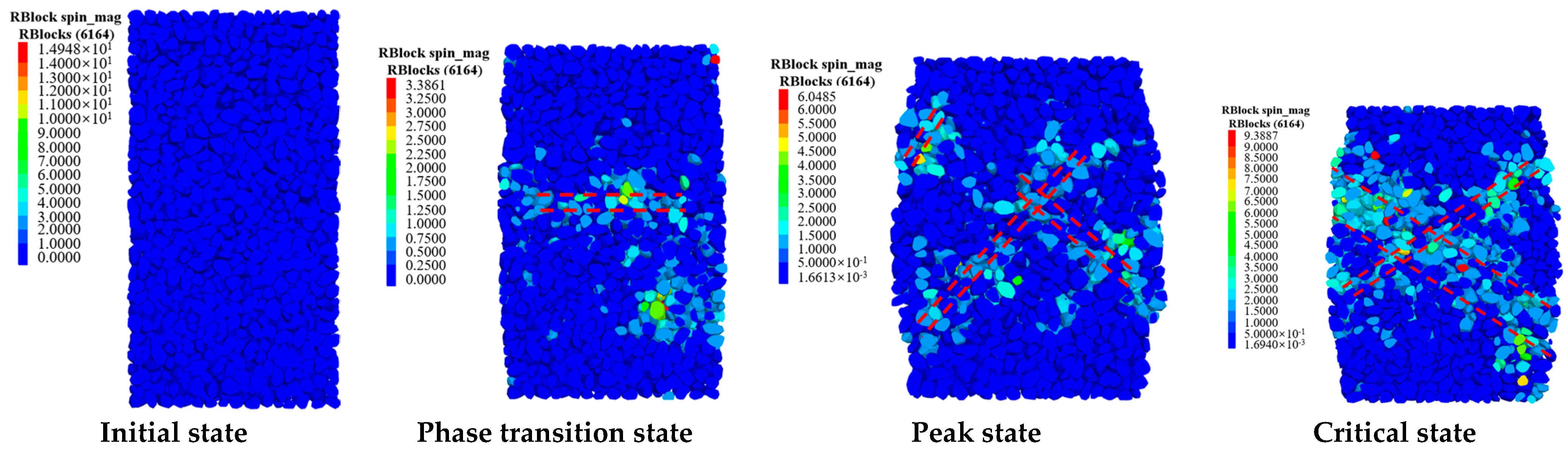
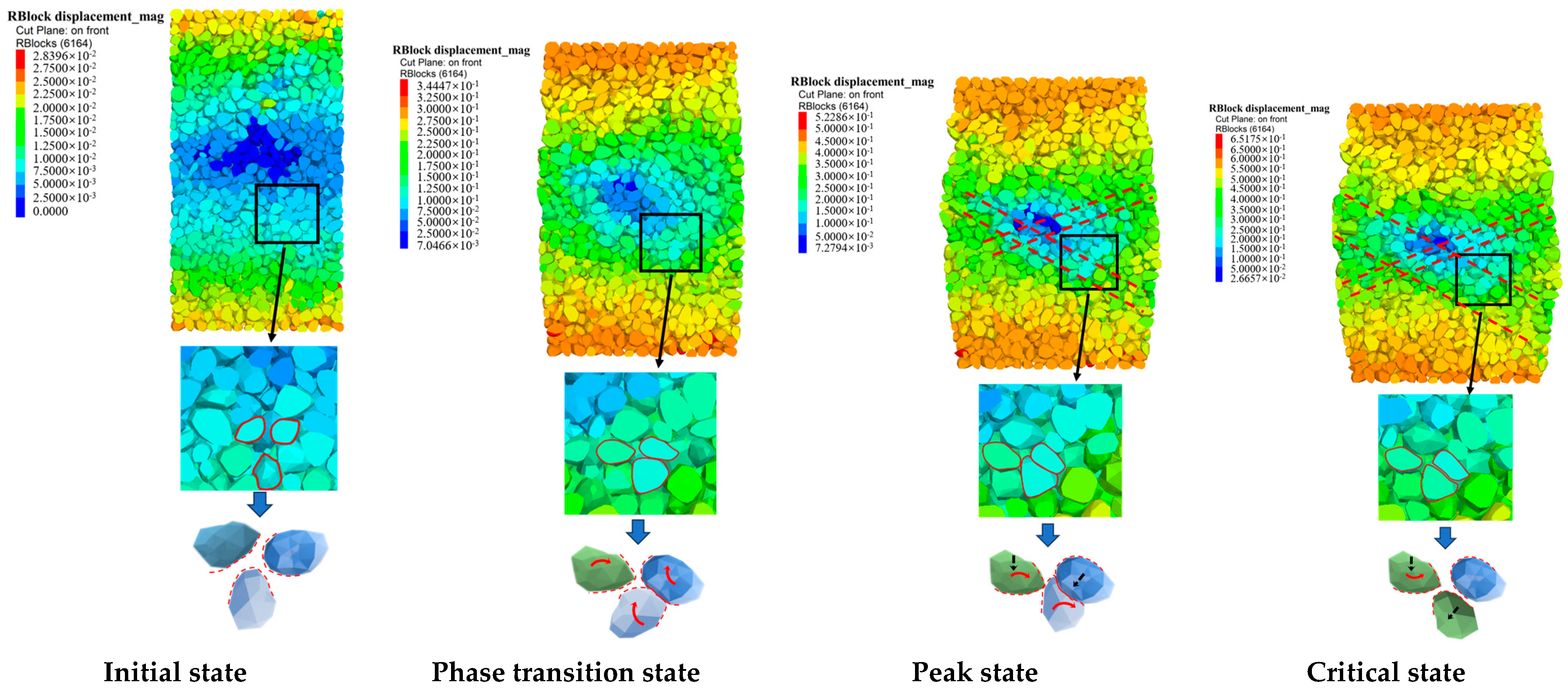
3.2.1. Flexible Boundary Displacement Shear Zone

Figure 9 shows the displacement cloud of the shell unit nodes on the flexible boundary of the stress-strain softening curve specimen. As shown in Figure 9, combined with the macro-mechanical characterization, the initial state, phase transition state, peak state, and critical state were taken to analyze the four states. The trend of the specimen displacement of the flexible boundary for the upper and lower parts of the displacement is large, the middle displacement is small, the trend of lateral deformation occurs in the phase transition state, the amount of displacement gradually increases, and the lateral deformation reaches the maximum value in the critical state, which presents a bulging damage pattern. Figure 10 shows the rotation process of the particles inside the stress-strain softening curve specimen, and the red dashed line in the figure marks the shear zone. As shown in Figure 10, when the specimen is in the initial state, due to the influence of the upper and lower wall stresses, elastic deformation occurs at this stage, the particles are mainly extruded from each other, the specimen is compacted, there is no obvious rotational deformation, and macroscopic compaction manifests as shear shrinkage deformation. With loading, the loading effect on the particles gradually increased, and the particles at different positions underwent different degrees of rotational deformation, particle position adjustment, and rearrangement. At this time, the macroscopic volumetric strain changed from compression to expansion, and the specimen entered a phase change state and exhibited a shear expansion trend, but the rotational deformation of the particles was still not obvious. When the axial strain reaches approximately 9%, the stress level reaches its peak, the specimen enters its peak state, the rotational angle between the particles increases, and the rotational angle is constantly adjusted to move to the beginning of the occurrence of misalignment and overrun. In the middle of the specimen, uneven bulging occurs, and the regularity of the arrangement of the particles becomes increasingly obvious, leading to localized regionalization and the formation of a staggered shear zone. When the specimen enters the critical state, the rotational deformation between the particles reaches the extreme value, forming an “X”-shaped shear band starting from the two ends of the specimen [24]. At this time, the shear strength of the specimen is reduced, and there is an obvious bulging deformation. Combined with the macroscopic triaxial test (stress-strain curve results), it can be concluded that a shear band is fully formed when the specimen reaches the peak stress after the strain softening stage.

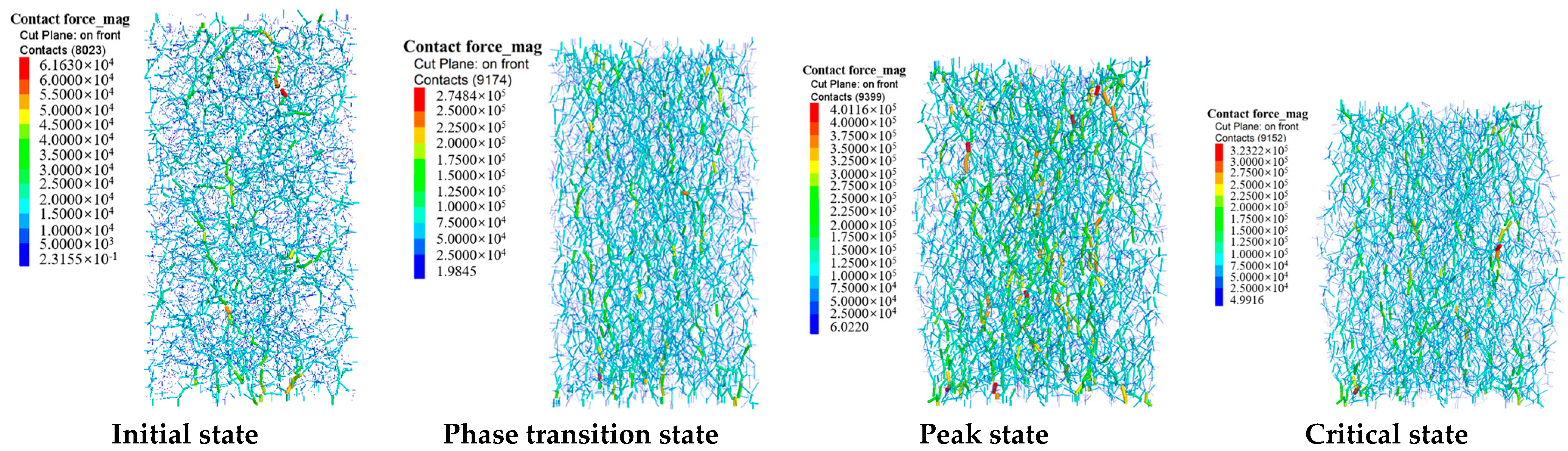
3.2.2. Contact Force Chain

Figure 11 shows the formation of the contact force chain of the specimen with a stress-strain softening curve. As shown in Figure 11, in the initial state, the contact force chain between the particles inside the specimen is uniformly distributed, the overall strength of the contact force chain is low, and there is no distinction between strong and weak force chains. With loading, under the influence of axial load, the interaction force between particles gradually increased. Part of the strong force chain gradually appeared in the contact force chain of the specimen, which was manifested as the coarsening of the force chain, and the direction of the contact force chain was parallel to the axial load [19]. At the same time, a part of the force chain perpendicular to the direction of the axial load appeared in the middle of the specimen. At this time, there was a tendency for macroscopic shear expansion and deformation of the specimen. The specimen’s internal contact force chain structure is continuously adjusted to resist the load. When the specimen reaches the peak state, the strength of the internal force chain of the specimen also reaches the peak, the strong and weak force chains in the force chain system are clearly distinguished, the strong force chain in the vertical direction is especially obvious, and the number of force chains increases. With increasing specimen shear damage, the strength of the force chain decreased, while the number of force chains decreased compared with that in the previous period, and the overall performance first increased and then decreased. At this time, the specimen reaches the critical state, the macroscopic stress and body change tend to stabilize and no longer undergo large changes, and the contact force chain structure between the particles is also basically stable, indicating that the evolution of the internal particle structure of the specimen tends to be stable.

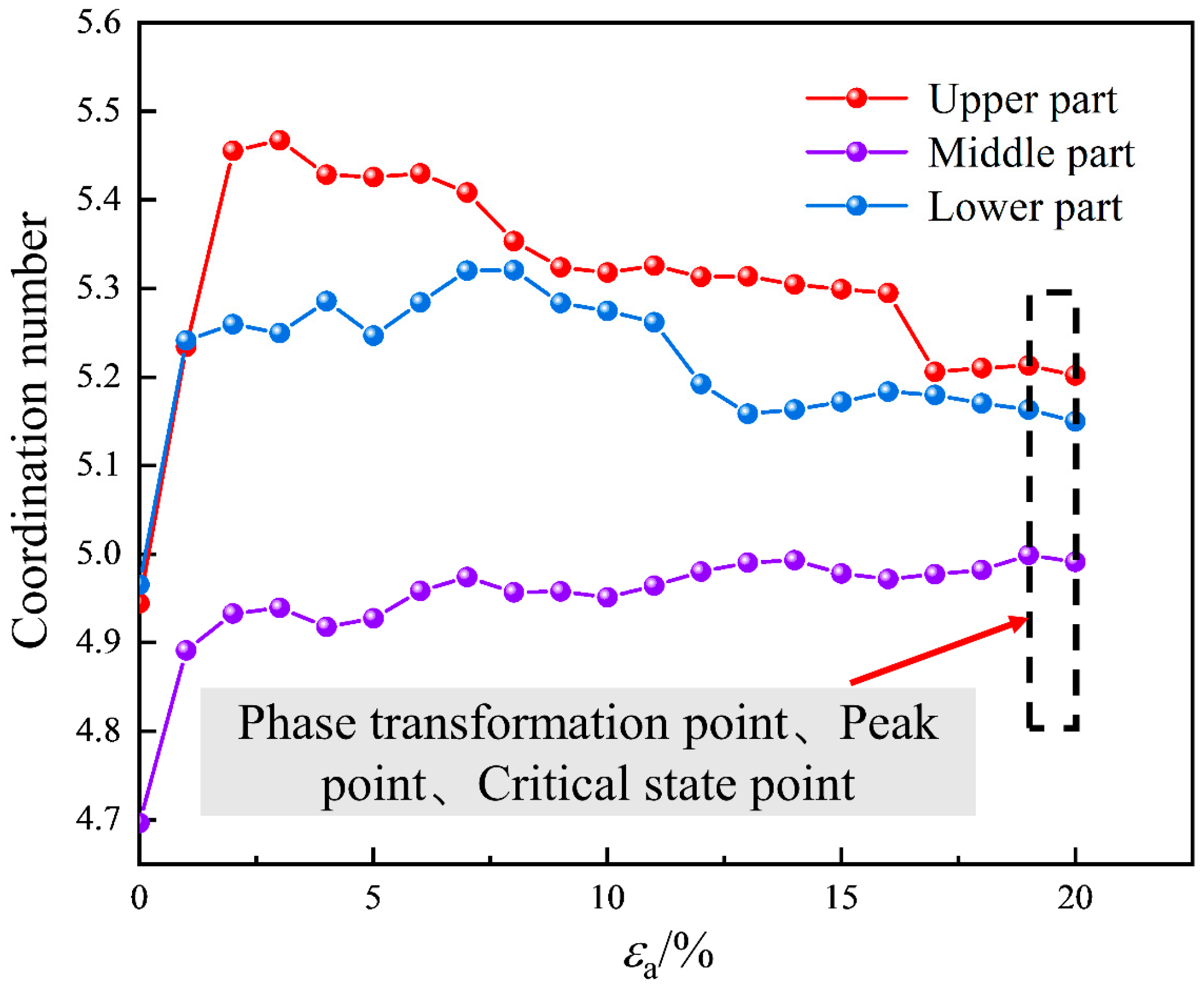
3.2.3. Coordination Number

Figure 12 shows the evolution of the coordination number in different regions of the stress-strain softening curve specimen, with the center of the specimen shape as the center, in the center of the shape and its upper and lower sides to set a measurement circle to detect the evolution of the coordination number. As shown in Figure 12, the coordination numbers at different locations inside the specimen are basically the same in the initial state, and with increasing loading, the coordination number increases significantly. Then, the specimen is further compressed and densified, and the coordination number reaches an extreme value when it reaches the phase transition point. At the same time, the coordination number in the middle part of the specimen is lower than that in the upper and lower parts, i.e., the number of contacts between the middle part of the specimen is lower than that between the upper and lower parts. This is because the specimen is in the phase transition state, the internal particles are rotationally deformed, and the particles in the middle of the specimen tend to expand to both sides, which is manifested as shear deformation. When the specimen reaches the peak state, the internal coordination number of the specimen decreases compared with that of the phase transition state, and the specimen macroscopically shows more significant shear deformation. With increasing loading, the decrease in the coordination number slows and finally stabilizes, but the increase in the coordination number of the upper and lower parts is still greater than that in the middle. Zhang P et al. concluded that at low perimeter pressures and high densities, the specimen coordination number stabilized after a gradual decrease after the peak as loading progressed [31]. Compared with Figure 10, it can be seen that the middle part of the specimen appears to have a large rotational angle, high porosity of the “X”-shaped shear zone, and large shear distortion deformation. The macroscopic deformation of the specimen can be reflected by the change in the coordination number; the increase in the coordination number shows the shear shrinkage phenomenon, and the decrease in the coordination number shows the shear expansion phenomenon.

3.3. Analysis of the Microscopic-Scale Evolution of Stress-Strain Hardening Type Curves

3.3.1. Flexible Boundary Displacement Shear Zone

Figure 13 shows the displacement cloud of the shell unit nodes on the flexible boundary of the specimen with a stress-strain hardening curve. As shown in Figure 13, the displacement trend of the specimen is similar to that of the softening type curve, as the upper and lower parts of the displacement are large in the middle of the displacement curve, but the difference is that more obvious lateral deformation did not occur, and a bulge phenomenon did not appear. The flexible membrane shrinks inwardly close to the heap stone particles, which is macroscopically manifested as shear shrinkage. Figure 14 shows the rotational process of the particles inside the stress-strain hardening curve specimen. As shown in Figure 14, there was no obvious rotational deformation inside the particles in the initial state, and the specimen was compressed densely from a macroscopic point of view, which showed the phenomenon of shear shrinkage. With the loading process, the upper and lower ends and the middle part of the specimen showed some rotational deformation, and the position of the particles was adjusted to a small extent. During the subsequent loading process, the particles in the middle of the specimen continued to undergo rotational deformation but did not undergo structural adjustment until the end of the loading shear band had never formed. Macroscopically, the shear strength of the specimen increases with increasing axial strain and does not reach the damage point at the end of the shear, and the stress-strain curve exhibits a strain hardening phenomenon. With increasing confining pressure, in the shear process, it becomes more difficult for the specimen to form a shear band, and under the high confining pressure, the so-called “shear band” is made up of a large number of cracks that do not penetrate the composition of the cracks and are still present in the shear strength. The macro stress-strain curve shows strain hardening characteristics and a low confining pressure under the phenomenon of strain softening is caused by the formation of the shear band.

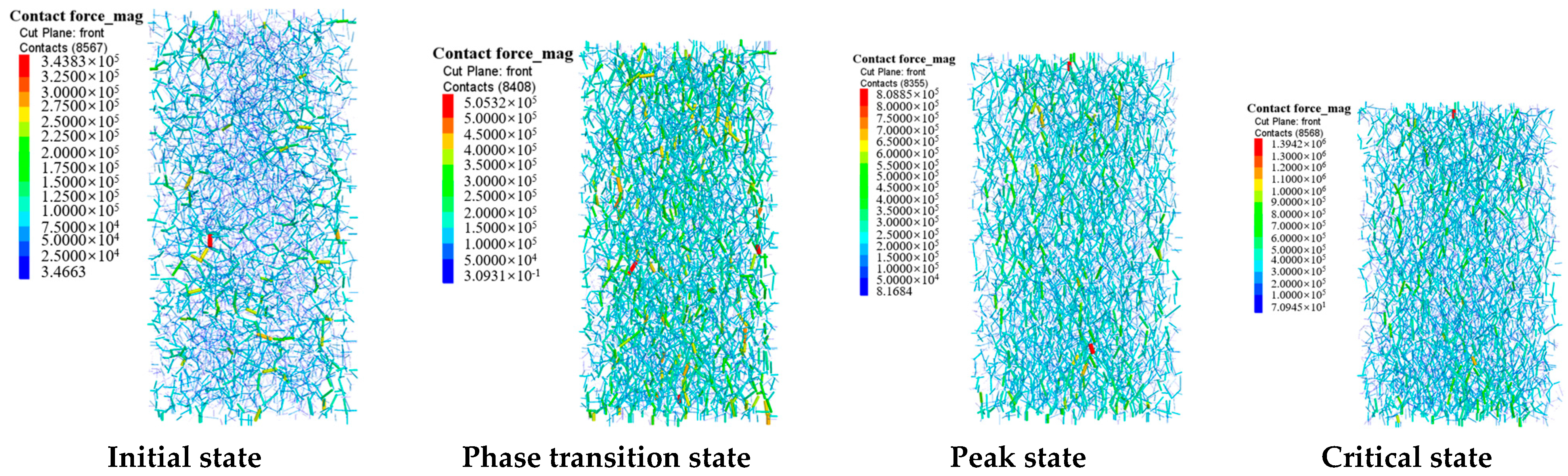
3.3.2. Contact Force Chain

Figure 15 shows the formation of the contact force chain of the specimen with a stress-strain hardening curve. As shown in Figure 15, the contact force chains between the particles inside the specimen in the initial state are uniformly distributed, the strength of the force chain decreases overall, and there is no strong force chain. With loading, the number of particles gradually increased due to the axial load, part of the force chain broke, the direction of the force chain became parallel to the axial load, the contact force between the particles became larger, the force chain morphology became more obvious, and there was a more significant strong chain. When the axial strain reaches 9%, the force chain strength is still in the ascending stage, the strength of the force chain continues to increase, and the strong force chain has a significant vertical distribution in the specimen. By the end of loading, the strength of the force chain continued to increase, the strong and weak force chains were clearly distinguishable, while the weak force chains gradually accumulated around the strong force chains and formed a large frictional resistance, which was reflected in the peak strength of the stress-strain curve after the hardening phenomenon. The above phenomenon is mainly due to the increase in the degree of compactness of the particle arrangement. The contact between the particles increases, and the ability of the specimen to resist the shear action also gradually increases, macroscopically manifesting as a higher strength. However, a large number of cracks can also be uniformly distributed inside the specimen because it is difficult to form a shear band under high confining pressure.

3.3.3. Coordination Number

Figure 16 shows the evolution of the coordination number in different regions of the stress-strain hardening curve specimen. Figure 16 shows that the initial stage of the specimen in the middle of the specimen is lower than the upper and lower parts of the coordination number level, which is due to the precompression of the specimen before the loading treatment so that the internal particles of the specimen release the internal stresses and the overall equilibrium is reached. As the loading progresses, the coordination number increases significantly when the loading compacts the specimen, and the number of contacts between the internal particles increases. After that, by the end of loading, the coordination number slightly decreased and then stabilized, and the coordination number in the middle part of the specimen was obviously lower than that in the upper and lower parts. Xu M et al. reached a similar conclusion [39]. Compared with Figure 13, it can be seen that the specimen macroscopically showed shear deformation, and the specimen was constantly compressed tightly, which made the number of interparticle contacts increase significantly. At the same time, Figure 14 shows that the middle part of the specimen was destroyed mainly by fissures, and the fissures produced between the specimens led to the destruction of the contact between the specimens. With respect to the contact damage, the coordination number slightly decreased, but compared with that in the initial state, it was still high. According to the change in the coordination number, the specimen macroscopically exhibited shear shrinkage hardening.

4. Discussion

Existing studies have indicated [11,40] that the mechanical properties of rockfill materials are closely related to the degree of compactness and perimeter pressure, and as an important basis for evaluating the structural stability of rockfill materials in engineering, it is necessary to consider the influence of density and confining pressure on the mechanical properties and deformation characteristics of rockfill materials. Some scholars have investigated the macro-mechanical characteristics of rockfill materials under the influence of density and confining pressure and their internal evolution mechanism via physical tests and numerical simulations. Although scholars have explored the microscopic characteristics of rockfill materials under different densities, which are difficult to measure by physical tests, based on the DEM, these studies are still mostly based on the reduction of physical tests, which do not provide a better explanation of the evolution law of microscopic structures. Relying on the coupling technology of discrete element and finite element methods, this paper carries out a large-scale triaxial numerical simulation test of rockfill materials to explore the influence of different densities and confining pressures on the mechanical behavior of rockfill materials and to reveal the mechanism of fine deformation damage, and preliminary results were obtained. Compared with previous studies, this paper further describes the microscopic mechanism under macroscopic characterization, provides a reference for explaining the intrinsic influence mechanism of density and confining pressure on the mechanical properties of rockfill materials, compares the macroscopic and microscopic changes in the initial, shear expansion, peak, and critical states, analyzes the mechanism, and discusses the discovery of a close link between the macroscopic mechanical properties and the microscopic grained group structural evolution of rockfill materials.

For the stress-strain softening type curve, the macroscopic performance for the initial state of the specimen is relatively loose. With the application of an axial load, the specimen is compacted with a small magnitude of shear shrinkage deformation, the deviatoric stress gradually increases, and the phase transition state shows a tendency toward shear distension deformation. The peak state of the deviatoric stress to reach the extreme value of the specimen shear distension deformation becomes more significant. Then, the deviatoric stress begins to decrease to the critical state and tends to stabilize. The specimen shows significant shear expansion and softening deformation [13]. Figure 17 shows the internal deformation mechanism of the specimen with a stress-strain softening curve, which is represented by the particle displacement cloud. As shown in Figure 17, in the initial state, the number of pores between the particles is large, the number of contacts is small, and the particles have a small effect on the deformation of the specimen. With increasing loading, the number of pores between the particles decreases due to the axial load, but the energy provided by the load is not sufficient to compact all the pores between the particles; thus, the specimen soon enters a phase transition state, and the particles squeeze each other with misalignments, rotations and other behaviors that lead to some degree of shear deformation. The load between the particles continues to increase, and the particle displacement cloud deforms the middle part of the specimen. With a certain degree of shear deformation, the load between the particles continued to increase, the middle of the specimen particles began to expand outwardly, and the specimen reached the peak state when the shear deformation became more significant. In the peak state, the specimen could not continue to withstand the load deformation generated by the destruction of the middle of the particles, the middle of the particles underwent greater movement and deformation, but the upper and lower parts of the specimen were still in close contact, resulting in significant bulging deformation of the specimen.

For the stress-strain hardening type curve, the macroscopic performance of the initial state is similar to that of the softening type curve and is relatively loose. With the application of an axial load, the specimen is compacted, and a shear shrinkage phenomenon occurs. Afterward, the deviatoric stress continues to increase until the end of the loading specimen reaches the shear shrinkage deformation state, the specimen does not appear to tend to expand the deformation, and a clear distinction between the phase transition, the peak value and the critical state is not observed [41]. Figure 18 shows the internal deformation mechanism of the stress-strain hardening curve specimen. As shown in Figure 18, the contact between the particles in the initial state is limited, and the effect on the deformation of the specimen is also small. When the specimen’s stress-strain softening curve is different, the axial load is greater at this time. Under the action of axial loading, the pore space between the particles continues to decrease, and the energy provided by the load is able to compact the interparticle porosity, so the specimen has always exhibited shear shrinkage behavior that does not appear in a state of phase transition; until the end of the load, the particles within the specimen exhibit only a small range of displacement. Until the end of the loading, the particles in the specimen exhibit only a small range of displacement and rotation, making the specimen increasingly compact. The volume gradually shrinks, the ability to withstand the load continues to increase, and the macroscopic shear strength of the specimen increases, which is manifested as shear deformation.

Moreover, we must recognize the assumptions established during the numerical simulation. Although the influence of the shape of the rockfill material was considered by the rblock unit, the particle-crushing effect it exhibits under high confining pressure was not considered in this paper. Therefore, in subsequent studies, a flexible cluster unit that can be crushed can be established by improving the algorithm, and the influence of the particle crushing effect on the characteristic state of the rockfill material and the evolution of the fine-grained group structure can be simulated under high confining pressure.

5. Conclusions

In this paper, a large triaxial numerical simulation test under different densities is carried out with rockfill materials as the research object, and the deformation and damage laws of rockfill materials in the initial, phase transition, peak, and critical states are analyzed from macroscopic and microscopic points of view. The following conclusions are drawn:

(1)

The stress-strain curve characteristics of rockfill materials can be divided into softening and hardening types. The softening type curve shows different mechanical properties in the initial, phase transition, peak, and critical states, resulting in significant shear deformation. The hardening type curve in the loading process of deviatoric stress continues to increase, and there is no obvious distinction between the phase transition, peak, and critical states; at the same time, more significant shear shrinkage deformation is produced.

(2)

The softening curve in the fine view shows that the displacement of the upper and lower ends of the shell unit on the flexible boundary increases with increasing loading, and the displacement of the middle ends decreases; however, the rotational deformation of the particles in the middle part of the specimen increases, and there is an “X”-type shear band. The strength of the force chain tends to increase and subsequently decrease. The coordination number is closely related to the deformation of the specimen, and it tends to increase first and subsequently decrease. The coordination number is closely related to the deformation of the specimen, showing a tendency to increase and then decrease, which corresponds to the macroscopic deformation of the specimen of shear shrinkage and then shear expansion.

(3)

According to the fine view of the hardening curve, with the loading of the flexible boundary on the shell unit, the softening type curve is similar to the performance of the upper and lower ends of the displacement and is large in the middle of the displacement, but the overall displacement is small. Similarly, for the specimens in the middle of the rotational deformation and the emergence of more cleavage zones rather than shear zones, the strength of the force chain continues to increase, and the coordination number of the first increases and then tends to stabilize, corresponding to macroscopic shear shrinkage deformation of the specimen.

References

1. Göncü, F.; Luding, S. Effect of particle friction and polydispersity on the macroscopic stress—Strain relations of granular materials. Acta Geotech. 2013, 8, 629–643. [Google Scholar] [CrossRef]
2. Pietruszczak, S.; Guo, P. Description of deformation process in inherently anisotropic granular materials. Int. J. Numer. Anal. Methods Geomech. 2013, 37, 478–490. [Google Scholar] [CrossRef]
3. Wan, R.G.; Guo, P.J. A simple constitutive model for granular soils: Modified stress-dilatancy approach. Comput. Geotech. 1998, 22, 109–133. [Google Scholar] [CrossRef]
4. Ishihara, K.; Tatsuoka, F.; Yasuda, S. Undrained deformation and liquefaction of sand under cyclic stresses. Soils Found. 1975, 15, 29–44. [Google Scholar] [CrossRef]
5. Liu, J.M.; Zou, D.G.; Kong, X.J.; Liu, H.B. Stress-dilatancy of Zipingpu gravel in triaxial compression tests. Sci. China Technol. Sci. 2016, 59, 214–224. [Google Scholar] [CrossRef]
6. Kong, X.; Liu, J.; Zou, D.; Liu, H.B. Stress-dilatancy relationship of Zipingpu gravel under cyclic loading in triaxial stress states. Int. J. Geomech. 2016, 16, 04016001. [Google Scholar] [CrossRef]
7. Luong, M.P. Stress-strain aspects of cohesionless soils under cyclic and transient loading. In Proceedings of the International Symposium on Soils under Cyclic and Transient Loading, Rotterdam, The Netherlands, 7–11 January 1980; Volume 1, pp. 315–324. [Google Scholar]
8. Xiao, Y.; Liu, H.; Liu, H.; Chen, Y.M.; Zhang, W.G. Strength and dilatancy behaviors of dense modeled rockfill material in general stress space. Int. J. Geomech. 2016, 16, 04016015. [Google Scholar] [CrossRef]
9. Roscoe, K.H.; Schofield, A.N.; Wroth, C.P. On the yielding of soils. Geotechnique 1958, 8, 22–53. [Google Scholar] [CrossRef]
10. Yang, G.; Jiang, Y.; Nimbalkar, S. Influence of particle size distribution on the critical state of rockfill. Adv. Civ. Eng. 2019, 2019, 1–7. [Google Scholar] [CrossRef]
11. Ning, F.; Liu, J.; Kong, X. Critical state and grading evolution of rockfill material under different triaxial compression tests. Int. J. Geomech. 2020, 20, 04019154. [Google Scholar]
12. Xiao, Y.; Liu, H.; Chen, Y. State-dependent constitutive model for rockfill materials. Int. J. Geomech. 2015, 15, 04014075. [Google Scholar]
13. Yang, Z.X.; Wu, Y. Critical state for anisotropic granular materials: A discrete element perspective. Int. J. Geomech. 2017, 17, 04016054. [Google Scholar] [CrossRef]
14. Cheng, J.; Ma, G.; Zhang, G. Deterioration of Mechanical Properties of Rockfill Materials Subjected to Cyclic Wetting–Drying and Wetting. Rock Mech. Rock Eng. 2023, 56, 2633–2647. [Google Scholar] [CrossRef]
15. Chang, W.J.; Phantachang, T. Effects of gravel content on shear resistance of gravelly soils. Eng. Geol. 2016, 207, 78–90. [Google Scholar] [CrossRef]
16. Liu, M.; Gao, Y.; Liu, H. An elastoplastic constitutive model for rockfills incorporating energy dissipation of nonlinear friction and particle breakage. Int. J. Numer. Anal. Methods Geomech. 2014, 38, 935–960. [Google Scholar] [CrossRef]
17. Mahinroosta, R.; Alizadeh, A.; Gatmiri, B. Simulation of collapse settlement of first filling in a high rockfill dam. Eng. Geol. 2015, 187, 32–44. [Google Scholar] [CrossRef]
18. Zhang, B.Y.; Zhang, J.H.; Sun, G.L. Deformation and shear strength of rockfill materials composed of soft siltstones subjected to stress, cyclical drying/wetting and temperature variations. Eng. Geol. 2015, 190, 87–97. [Google Scholar] [CrossRef]
19. Cundall, P.A.; Strack, O.D.L. A discrete numerical model for granular assemblies. Geotechnique 1979, 29, 47–65. [Google Scholar] [CrossRef]
20. Han, H.; Chen, W.; Huang, B. Numerical simulation of the influence of particle shape on the mechanical properties of rockfill materials. Eng. Comput. 2017, 34, 2228–2241. [Google Scholar] [CrossRef]
21. Zhou, W.; Ma, G.; Chang, X.L. Discrete modeling of rockfill materials considering the irregular shaped particles and their crushability. Eng. Comput. 2015, 32, 1104–1120. [Google Scholar] [CrossRef]
22. Zhang, R.; Zhang, L.; Shi, C. Microscopic mechanical properties of rockfill materials under different stress paths. Granul. Matter 2024, 26, 41. [Google Scholar] [CrossRef]
23. Xu, M.; Hong, J.; Song, E. DEM study on the effect of particle breakage on the macro-and micro-behavior of rockfill sheared along different stress paths. Comput. Geotech. 2017, 89, 113–127. [Google Scholar] [CrossRef]
24. Wu, K.; Sun, W.; Liu, S.; Zhang, X. Study of shear behavior of granular materials by 3D DEM simulation of the triaxial test in the membrane boundary condition. Adv. Powder Technol. 2021, 32, 1145–1156. [Google Scholar] [CrossRef]
25. Qu, T.; Feng, Y.T.; Wang, Y. Discrete element modelling of flexible membrane boundaries for triaxial tests. Comput. Geotech. 2019, 115, 103154. [Google Scholar] [CrossRef]
26. Cil, M.B.; Alshibli, K.A. 3D analysis of kinematic behavior of granular materials in triaxial testing using DEM with flexible membrane boundary. Acta Geotech. 2014, 9, 287–298. [Google Scholar] [CrossRef]
27. Zhou, W.; Liu, J.; Ma, G. Three-dimensional DEM investigation of critical state and dilatancy behaviors of granular materials. Acta Geotech. 2017, 12, 527–540. [Google Scholar] [CrossRef]
28. Cai, G.; Li, J.; Liu, S. Simulation of Triaxial Tests for Unsaturated Soils under a Tension–Shear State by the Discrete Element Method. Sustainability 2022, 14, 9122. [Google Scholar] [CrossRef]
29. Qin, Y.; Liu, C.; Zhang, X. A three-dimensional discrete element model of triaxial tests based on a new flexible membrane boundary. Sci. Rep. 2021, 11, 4753. [Google Scholar] [CrossRef] [PubMed]
30. Xiao, G.; Liu, S.; Zhang, Y.; Wu, Y.; Chen, B.; Song, S. A measurement method of the belt grinding allowance of hollow blades based on blue light scanning. Int. J. Adv. Manuf. Technol. 2021, 116, 3295–3303. [Google Scholar] [CrossRef]
31. Zhang, P.; Sun, X.; Zhou, X.; Zhang, Y. Experimental simulation and a reliable calibration method of rockfill microscopic parameters by considering flexible boundary. Powder Technol. 2022, 396, 279–290. [Google Scholar] [CrossRef]
32. Li, J.; Konietzky, H.; Frühwirt, T. Voronoi-based DEM simulation approach for sandstone considering grain structure and pore size. Rock Mech Rock Eng. 2017, 50, 2749–2761. [Google Scholar] [CrossRef]
33. Zhang, C.; Shi, C.; Wang, S.; Zhang, Y. Vibratory compaction properties of off-shore gravity quays rubble bed based on rigid blocks. Mar. Georesources Geotechnol. 2023, 41, 1–16. [Google Scholar] [CrossRef]
34. Shi, C.; Xu, W. Techniques and Practices for Numerical Simulation of Particle Flows; China Architecture & Building Press: Beijing, China, 2015; pp. 380–403. [Google Scholar]
35. Shi, C.; Li, W.; Meng, Q. A dynamic strain-rate-dependent contact model and its application in Hongshiyan landslide. Geofluids 2021, 2021, 1–23. [Google Scholar] [CrossRef]
36. Bu, P.; Li, Y.; Zhang, X. A calibration method of discrete element contact model parameters for bulk materials based on experimental design method. Powder Technol. 2023, 425, 118596. [Google Scholar] [CrossRef]
37. Ma, C.; Yang, J.; Zenz, G. Calibration of the microparameters of the discrete element method using a relevance vector machine and its application to rockfill materials. Adv. Eng. Soft. 2020, 147, 102833. [Google Scholar] [CrossRef]
38. Guo, W.L.; Cai, Z.Y.; Wu, Y.L.; Zhang, C. Dilatancy behavior of rockfill materials and its description. Eur. J. Environ. 2022, 26, 1883–1896. [Google Scholar] [CrossRef]
39. Xu, M.; Hong, J.; Song, E. DEM study on the macro-and micro-responses of granular materials subjected to creep and stress relaxation. Comput. Geotech. 2018, 102, 111–124. [Google Scholar] [CrossRef]
40. Pan, J.; Jiang, J.; Cheng, Z. Large-scale true triaxial test on stress-strain and strength properties of rockfill. Int. J. Geomech. 2020, 20, 04019146. [Google Scholar]
41. Wang, Y.; Cui, F. Energy evolution mechanism in process of Sandstone failure and energy strength criterion. Appl. Geophys. 2018, 154, 21–28. [Google Scholar] [CrossRef]
Figure 1. Virtual structural surface reconstruction process for blocks. (a) Three-dimensional scanning device; (b) original specimen; (c) surface point cloud; (d) point cloud noise reduction; (e) PFC particle modeling.
Applsci 14 04353 g001
Figure 2. Linear model. (a) Linear model behavior; (b) local coordinate system on the contact plane; (c) contact force and its components; (d) force–displacement theorem for linear model components.
Applsci 14 04353 g002
Figure 3. Large triaxial test device. (a) Large-scale triaxial apparatus; (b) specimen.
Applsci 14 04353 g003
Figure 4. Comparison of the gradation curves between the indoor test and simulation test results.
Applsci 14 04353 g004
Figure 5. Schematic diagram of the numerical model: (a) numerical model; (b) model volumetric strain calculation.
Applsci 14 04353 g005
Figure 6. Laboratory test and numerical simulation curve.
Applsci 14 04353 g006
Figure 7. Deviatoric stress and volumetric strain versus axial strain curves of specimens under different confining pressures. (a) Deviatoric stress-axial strain curve; (b) volumetric strain-axial strain curve.
Applsci 14 04353 g007
Figure 8. Deviatoric stress and volumetric strain versus axial strain curves of specimens with different compactness. (a) Deviatoric stress-axial strain curve; (b) volumetric strain-axial strain curve.
Applsci 14 04353 g008
Figure 9. Displacement cloud of shell unit nodes on the flexible boundary of the specimen (stress-strain softening curve).
Applsci 14 04353 g009
Figure 10. The particle rotation process in the specimen (stress-strain softening curve).
Applsci 14 04353 g010
Figure 11. Evolution of the contact force chain inside the specimen (stress-strain softening curve).
Applsci 14 04353 g011
Figure 12. Variation curves of the coordination number in different regions of the specimen (stress-strain softening curve).
Applsci 14 04353 g012
Figure 13. Displacement cloud of shell unit nodes on the flexible boundary of the specimen (stress-strain hardening type).
Applsci 14 04353 g013
Figure 14. The particle rotation process in the specimen (stress-strain hardening type).
Applsci 14 04353 g014
Figure 15. Evolution of the contact force chain inside the specimen (stress-strain hardening type).
Applsci 14 04353 g015
Figure 16. Variation curves of the coordination number in different regions of the specimen (stress-strain hardening type).
Applsci 14 04353 g016
Figure 17. Diagram of the internal deformation mechanism of the specimen (stress-strain softening curve).
Applsci 14 04353 g017
Figure 18. Diagram of the internal deformation mechanism of the specimen (stress-strain hardening type).
Applsci 14 04353 g018