A Comparison of the Relationship between Dynamic and Static Rock Mechanical Parameters

Abstract

The rock’s mechanical properties play an important role in the whole process of conventional and unconventional oil and gas exploration and progression. At present, there are two approaches to determining the mechanical parameters. One is to measure the rock sample in the laboratory (i.e., static elastic modulus E_s). The other is to obtain parameters by geophysical logging data (i.e., dynamic elastic modulus E_d). In general, static parameters can more accurately reflect the mechanical properties of rock under actual geo-stresses. At the same time, their determinations are difficult. Therefore, one of the best methods is to establish the correlation between the dynamic and static parameters. This paper investigates the relation between the dynamic and static parameters using different methods for various rocks in the literature. Based on the relationship of $E_{\mathrm{s}}=\mathrm{a}{E}_{\mathrm{d}}+\mathrm{b}$, a correction between a and b is proposed using the multinomial form $\mathrm{a}=0.67+0.101\mathrm{b}-0.006{\mathrm{b}}^2+0.0001{\mathrm{b}}^3$. It is found that the E_s can be derived from the E_d just when the parameter b is known. In terms of different types of rocks, for igneous and metamorphic rocks, the best correlation between E_s and E_d obeys the power-law correlation; for sedimentary rocks, there are linear and logarithmic correlations. Theoretically, the difference between dynamic and static elastic moduli can be attributed to microcracks and pores within rocks. This study can provide guidance for engineers to predict the desired static parameters precisely using logging or seismic data.

1. Introduction

The mechanical properties of formation rocks are the foundation of oil/gas engineering design and development, during which these issues hinder the oil/gas recovery effect and safety a great deal, such as in the stability of wellbore, pay zones, and cap rocks, and the surface subsidence/uplift. For instance, the constitutive model can control the wellbore stability and reservoir compression/expansion capacity. Rock strength parameters can determine the reservoir stability and well drilling stability. The deformation parameters describing stress–strain behaviors, such as the elastic modulus (E) and Poisson’s ratio (μ), can impact the surface subsidence or uplift, and the safety of underground structures in exploration areas. In addition, these mechanical parameters above can not only play a critical role in the concentration, dispersion, propagation, and attenuation of geo-stress but also can provide an indispensable basis for the well drilling, well completion, and the numerical simulation of geo-mechanical stimulation in oil and gas reservoirs [1,2].

To date, the commonly used test methods of rock mechanical parameters include static and dynamic methods [3]. The static parameters can be obtained by measuring the degree of deformation of the rock sample under static loading, and the dynamic parameters can be obtained from the conversion of the ultrasonic propagation speed in the rock sample. The static test method is limited by the number of core wells and the cost, so the experimental data are limited. Although the static method is relatively accurate, the process is complex, costly, and requires specific downhole test equipment. Dynamic test methods (e.g., logging and seismic surveys) can obtain the continuous rock dynamic mechanical parameters along the depth, and the acquisition is convenient, economical, and reliable, so the dynamic method can usually overcome these shortcomings of the static method. However, taking the elastic modulus (E) as an instance, there is a challenging and meaningful study on the relation between static and dynamic elastic moduli. The earliest suggestion that there is a discrepancy between the dynamic (E_d) and static (E_s) elastic moduli was made by Zisman [4] at Harvard University. After that, many researchers conducted some experimental or analytical studies, and most of the results showed that the dynamic elastic modulus (E_d) is larger than the static elastic modulus (E_s) [5,6,7,8,9,10,11,12,13,14]. There is an acceptable linear or nonlinear relationship between the dynamic (E_d) and static (E_s) elastic moduli. The dynamic elastic moduli can reach 1 to 10 times the static elastic moduli. There is no obvious relationship between the dynamic (μ_d) and static (μ_s) Poisson’s ratios. While there is a relationship between dynamic and static parameters, the substantial variations in their data are primarily influenced by several complex factors. The external factors include the amount of stress, strain amplitude, test confining pressure, test temperature, and the test frequency of the rock sample [15,16,17]. The internal factors are mainly the mineral composition, content, pore development degree, microfractures or microcracks, pore fluid, coupling between rock particles, cementation type, and anisotropy of rock [3,6,18]. The discrepancy between dynamic (E_d) and static (E_s) elastic moduli has been extensively addressed in rock engineering, and this difference can typically be attributed to microcracks and pores within the rocks.

Because static test conditions are closer to the actual underground environments of rock [19], the static elastic parameters are frequently employed in practical engineering applications and can reflect formation properties more accurately [20,21,22,23]. In general, oil and gas field engineers hope to predict static mechanical parameters through dynamic mechanical parameters. Therefore, one of the best methods is to use the experimental and logging data to obtain the dynamic–static conversion relationship. The three procedures are as follows: use present data to draw an intersection diagram (dynamic parameter as X-axis and static parameter as Y-axis); obtain relation equations between dynamic and static parameters; and predict the static parameter according to the dynamic–static conversion relation in the study area. In this regard, the method above can obtain a continuous rock static mechanics parameter profile of the well and promote the application to other wells in the study area, providing a reliable basis for oil/gas exploration and development as well as drilling engineering design. So far, several formulas have been developed to establish the correlation that exists between static and dynamic elastic moduli. The empirical equations between dynamic (E_d) and static (E_s) elastic moduli of rocks have been studied by the Institute of former Yugoslavia and the Institute of Geology and Geophysics in Belgrade. Utilizing a large number of comparative studies on experimental data, the Institute of Geology of the Chinese Academy of Sciences proposed a linear correlation for the estimate of static elastic modulus from dynamic elastic modulus. However, this equation is only suitable for microcline and granite [7,8,9,24,25,26,27,28,29]. King [7] established a linear correlation between the dynamic and static parameters of igneous and metamorphic rocks. McCann and Entwisle [30] established linear dynamic–static relations for several types of rocks. In addition, some other conversion equations were employed for various rocks [10,31]. Martinez et al. [32] conducted laboratory experiments on ten carbonate rocks extracted from Spain and established different conversion correlations. Brotons et al. [33] showed linear and nonlinear correlations for different rock types. However, the applicability of each of these correlations is limited to the type of rock (igneous, metamorphic, and sedimentary rocks) under particular conditions.

Therefore, this paper aims to review the correlation between dynamic and static parameters of various geological formations in other regions and use acoustic tools such as acoustic logging, seismic data, and indoor ultrasonic testing to speculate on the static parameters.

2. Testing of Dynamic and Static Elastic Parameters

The mechanical parameters of rock (Poisson’s ratio and elastic modulus, etc.) are the basis of petroleum engineering exploration and development design. At present, there are two approaches to determining the mechanical parameters. One is the dynamic rock mechanical parameter (i.e., dynamic elastic modulus), which can be acquired by downhole tests, such as wave logging and seismic data. The other is the static rock mechanical parameter measured by the uniaxial and triaxial experiments in the laboratory (i.e., static elastic modulus). Static elastic modulus is an important parameter in drilling, completion, and fracturing. According to the characteristics of underground engineering, the static elastic parameters of rock should be used in practical engineering. It is necessary to convert the dynamic elastic parameters of log calculation into static elastic parameters for the convenience of the application. However, the static elastic parameters of the rock can only be obtained by extracting the core from the ground and testing it in the laboratory, which is time consuming and expensive. To obtain the real static elastic parameters under the reservoir conditions, it is necessary to simulate the temperature and pressure conditions under the reservoir, which is more expensive and often requires a lot of core experimental data to accurately describe the mechanical characteristics of the reservoir. Therefore, the best method is to establish the transformation relationship between static and dynamic parameters. We can use acoustic tools such as acoustic logging, seismic data, and indoor ultrasonic testing to predict the static parameters of rock mechanics. It provides a way to obtain the mechanical property parameters of rock.

2.1. Static Elastic Parameter Acquisition Method

The static elastic modulus can be obtained by using rock samples to conduct the laboratory’s uniaxial or triaxial static loading experiments. In the experiment, maintaining a constant confining pressure under formation conditions by applying axial stress until the rock sample breakage and recording the deformation parameters during the experiment, a corresponding stress–strain curve is formed throughout the entire process [34,35]. Thus, the curve can directly give stress values, longitudinal strain, transverse strain, and deformation parameters. The deformation parameters obtained through compression tests are analyzed using regression analysis. The slope of the straight section on the stress–strain curve is taken as the static elastic modulus, and the static Poisson’s ratio is obtained according to the ratio of transverse deformation to longitudinal deformation of the rock sample. The elastic modulus is measured within the elastic limits. When rocks treated as an elastic body undergo elongation/compression deformation, the elastic modulus is the ratio of the tensile/compression stress to the relative elongation/shortening in the same direction, the ratio of applied stress to strain (stress in the same direction). Poisson’s ratio is measured when a rock sample is under tensile stress, causing elongation in the direction of the applied force and contraction in the direction perpendicular to the applied force. The ratio of transverse linear strain (contraction) to longitudinal linear strain (elongation) is known as Poisson’s ratio [36]. The slope on the stress–strain curve can obtain different types of static elastic modulus. The International Society of Rock Mechanics (ISRM) has proposed three standard measurement methods [37]. They are as follows: tangent elastic modulus (E_tan) is the slope of a tangent line at any point on the stress–strain curve. This is defined as the tangent slope of the stress–strain curve at a fixed percentage of the ultimate strength, as in Figure 1a; the average elastic modulus (E_ave) is the slope of a straight line portion of the stress–strain curve, as in Figure 1b; and secant elastic modulus (E_sec) is the slope of a straight line drawn from the origin (0,0) to the point on the curve that corresponds to some fixed percentage of the ultimate strength slope of the straight line plotted in Figure 1c [38]. This article adopts the tangent elastic modulus.

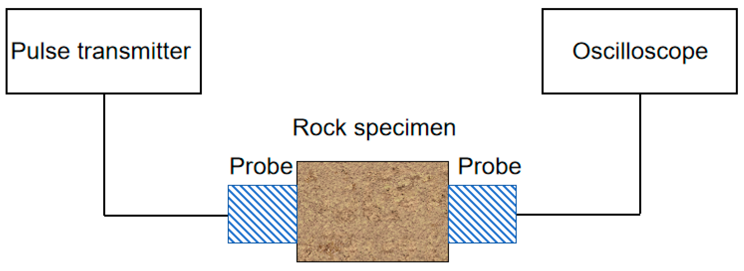
2.2. Dynamic Elastic Parameter Acquisition Method

There are two methods for determining the dynamic elastic parameters. One is to use logging equipment to conduct on-site sonic logging under geo-stress conditions, then convert the rock acoustic wave data (P-wave and S-wave time differences) and rock bulk density to obtain the elastic parameters of the rock formations continuously along the well depth. The calculation method is shown in Equations (1) and (2).

$$E_{\mathrm{d}}=\frac{{\rho }_{bulk}\left(3\Delta t_{\mathrm{s}}^2-4\Delta t_{\mathrm{p}}^2\right)}{\Delta t_{\mathrm{s}}^2\left(\Delta t_{\mathrm{s}}^2-\Delta t_{\mathrm{p}}^2\right)}$$

(1)

$${\mu }_{\mathrm{d}}=\frac{\Delta t_{\mathrm{s}}^2-2\Delta t_{\mathrm{p}}^2}{2\left(\Delta t_{\mathrm{s}}^2-\Delta t_{\mathrm{p}}^2\right)}$$

(2)

where E_d is the dynamic elastic modulus, GPa; ρ_bulk is the bulk density, g/cm³; Δt_s is the P-wave time difference, μs/m; Δt_p is the S-wave time difference, μs/m; μ_d is the dynamic Poisson’s ratio, dimensionless.

The second method is to convert the speed of ultrasonic propagation in rock specimens through laboratory tests. Using the ultrasonic pulse transmission method to measure the P-wave and S-wave velocity of rock samples, the experimental principle is shown in Figure 2. First, connect the two probes and observe whether the jumping time of the received waveform on the oscilloscope is zero. If the starting point time does not return to zero, adjust the knob of the pulse position in the pulse source to set the starting point time to zero, and the oscilloscope can directly detect the time when the first wave arrives [36]. Based on the theory of elastic waves, Equations (3) and (4) can be used to determine the dynamic elastic modulus (E_d) and Poisson’s ratio (μ_d) of rocks [34].

$$E_{\mathrm{d}}=\frac{{\rho }_{bulk}{V}_{\mathrm{s}}^2\left(3V_{\mathrm{p}}^2-4V_{\mathrm{s}}^2\right)}{V_{\mathrm{p}}^2-V_{\mathrm{s}}^2}$$

(3)

$${\mu }_{\mathrm{d}}=\frac{V_{\mathrm{p}}^2-2V_{\mathrm{s}}^2}{2\left(V_p^2-V_{\mathrm{s}}^2\right)}$$

(4)

where ρ_bulk is the bulk density of the sample, the unit is g/cm³; V_p is the P-wave velocity, the unit is m/s; V_s is the S-wave velocity, the unit is m/s.

However, acquiring S-wave data in the actual well-logging data is complex and expensive. Thus, conventional well-logging lacks S-wave velocity data [40]. Therefore, the first dynamic testing method is generally used in practical applications.

2.3. Synchronized Testing Methods for Dynamic and Static Parameters

The synchronous testing apparatus used for the U.S. GCTS RTR1500 (GCTS, Tempe, AZ, USA) high-temperature and high-pressure triaxial rock mechanics test system is shown in Figure 3. The sample acoustic wave velocity is measured using the ultrasonic transmission method in the system. The system can simulate the highest temperature of 150 °C, a maximum loading confining pressure of 140 MPa, a maximum axial load of 1500 KN, and an axial loading frequency of 10 Hz; the maximum pore pressure can reach 140 MPa and a sample diameter of 25–100 mm.

The end faces of the test rock specimens are polished, and the samples are treated in a natural dry state. The rock samples sealed with heat-shrinkable sleeves are placed in a high-temperature and high-pressure triaxial chamber, and high-precision extensometers are installed on the samples to measure the longitudinal and transverse deformation. For rock static testing, the sample is first subjected to confining pressure (hydrostatic pressure) to a specific value and then heated to a set temperature. After stabilizing the confining pressure and temperature, axial stress (differential stress) is applied at an equal axial displacement rate until the specimen is destroyed. The rock hydrostatic parameters, compressive strength, elastic modulus, and Poisson’s ratio under the corresponding temperature and pressure conditions can be obtained by recording the axial stress, axial deformation, and transverse deformation data. When conducting the synchronous testing of rock statics and acoustic velocity, a pressure and temperature-resistant ultrasonic transmitter and receiver transducer (with a center frequency of 1 MHz) installed in a triaxial chamber is used instead of a conventional mechanical pressure head; during the process of measuring the static deformation of rocks, the P-wave and S-wave velocities are simultaneously measured by the ultrasonic system under the same temperature and stress variation conditions. The experiment simultaneously acquired rock static deformation data and P-wave and S-wave velocities under the same sample, temperature, and stress variation conditions [41]. Based on the measured P-wave and S-wave velocities, the rock dynamic mechanical parameters under the corresponding temperature and stress conditions are calculated, as shown in Equations (3) and (4).

Figure 3. High-pressure and high-temperature triaxial test system, GCTS RTR-1500 [42].

Figure 3. High-pressure and high-temperature triaxial test system, GCTS RTR-1500 [42].

3. Dynamic–Static Conversion Relationship

3.1. Methods

Establishing a dynamic–static conversion relationship is essential for accurately evaluating the rock mechanical characteristics of the formation using logging data and seismic survey data, which in turn provides a reliable petrophysical basis for petroleum engineering design and oil/gas exploration in the region. Based on the results of the P-wave and S-wave velocities, measurements obtained from the dynamic method test and combined with the bulk density were obtained from the weighing method of the rock specimens. The dynamic elastic modulus and dynamic Poisson’s ratio can be calculated by using Equations (3) and (4), and the static elastic modulus and static Poisson’s ratio were measured by the indoor stress-loading experiments. Through static parameters (stress loading experiment) and dynamic parameters (acoustic testing), using the principle of least squares, a polynomial regression analysis was performed to find the best fitting curve between the dynamic and static parameters of different rocks based on the significance of the polynomial.

3.2. Relation Establishment

Table 1. Relationship proposed by various authors between static (E_s) and dynamic (E_d) elastic moduli.

NO	Equation	Unit	R2	Rock Type	Reference
5	$E_{\mathrm{s}}=1.137E_{\mathrm{d}}-9.68$	GPa	0.92	Granite	Belikov et al. (1970) [29]
6	$E_{\mathrm{s}}=1.263E_{\mathrm{d}}-29.5$	GPa	0.82	Igneous–metamorphic	King (1983) [7]
7	$\begin{array}{l}{E}_{\mathrm{s}}=\mathrm{\alpha }{E_{\mathrm{d}}}^{\mathrm{\beta }},\mathrm{\alpha }\in 0.097\mathrm{\sim }0.152,\\ \mathrm{\beta }\in 1.38\sim 1.48\end{array}$	GPa	0.96–0.99	Sandstone–granite	Van Heerden (1987) [9]
8	$E_{\mathrm{s}}=0.64E_{\mathrm{d}}-0.32$	GPa	0.84	All types	Eissa and Kazi (1988) [10]
9	$E_{\mathrm{s}}=0.74E_{\mathrm{d}}-0.82$	GPa	0.84	All types	Eissa and Kazi (1988) [10]
10	${\log }_{10}{E}_{\mathrm{s}}=0.77{\log }_{10}\left({\rho }_{bulk}{E}_{\mathrm{d}}\right)+0.02$	GPa	0.96	Sedimentary	Eissa and Kazi (1988) [10]
11	$E_{\mathrm{s}}=0.69E_{\mathrm{d}}+6.40$	GPa	0.75	All types	McCann and Entwisle (1992) [30]
12	$E_{\mathrm{s}}=1.05E_{\mathrm{d}}-3.16$	GPa	0.99	Sedimentary	Christaras et al. (1994) [43]
13	$E_{\mathrm{s}}=0.83E_{\mathrm{d}}$	GPa	-	Goncrele	Neville (1995) [44]
14	$E_{\mathrm{s}}=1.25E_{\mathrm{d}}-19$	GPa	-	Structural design	CP110 (1972) [45]
15	$E_{\mathrm{s}}=0.018E_{\mathrm{d}}{ }^2+0.422E_{\mathrm{d}}$	MPsi	0.75	Sedimentary	Lacy (1997) [46]
16	$E_{\mathrm{s}}=0.0293E_{\mathrm{d}}{ }^2+0.4533E_{\mathrm{d}}$	MPsi	0.74	Sandstones	Lacy (1997) [46]
17	$E_{\mathrm{s}}=0.0428E_{\mathrm{d}}{ }^2+0.2334E_{\mathrm{d}}$	MPsi	0.93	Shales	Lacy (1997) [46]
18	$E_{\mathrm{s}}=0.2807E_{\mathrm{d}}$	GPa	0.60	Sedimentary	Brautigam et al. (1998) [47]
19	$E_{\mathrm{s}}=1.153E_{\mathrm{d}}-15.2$	GPa	-	Hard rocks (Es > 15 GPa)	Nur and Wang (1999) [48]
20	$E_{\mathrm{s}}=0.8069E_{\mathrm{d}}$	GPa	0.92	Composite resin	Helvatjoglu et al. (2006) [49]
21	$E_{\mathrm{s}}=0.7707E_{\mathrm{d}}-5854$	GPa	0.96	All types	Mokovciakova and Pandula (2003) [50]
22	$E_{\mathrm{s}}=e^{(0.0477E_{\mathrm{d}})}$	GPa	0.72	All types	Fahimifar and Soroush (2003) [51]
23	$E_{\mathrm{s}}=0.5087E_{\mathrm{d}}-0.6\times {10}^6$	Psi	0.60	Sandstone	Al-Tahini (2003) [52]
24	$E_{\mathrm{s}}=0.0158{\left(E_{\mathrm{d}}\right)}^{2.74}$	GPa	-	Shale	Ohen (2003) [53]
25	$E_{\mathrm{s}}=0.541E_{\mathrm{d}}+12.852$	GPa	0.60	Limestone	Ameen et al. (2009) [54]
26	$E_{\mathrm{s}}=0.867E_{\mathrm{d}}-2.085$	GPa	0.96	Sedimentary	Brotons et al. (2014) [55]
27	${\log }_{10}{E}_{\mathrm{s}}=1.275{\log }_{10}\left({\rho }_{bulk}{E}_{\mathrm{d}}\right)-4.714$	GPa	0.97	Sedimentary	Brotons et al. (2014) [55]
28	$E_{\mathrm{s}}=0.932E_{\mathrm{d}}-3.421$	GPa	0.97	All types	Brotons et al. (2016) [33]
29	${\log }_{10}{E}_{\mathrm{s}}=0.967{\log }_{10}\left({\rho }_{bulk}{E}_{\mathrm{d}}\right)-3.306$	GPa	0.99	All types	Brotons et al. (2016) [33]
30	$E_{\mathrm{s}}=0.014{E_{\mathrm{d}}}^{1.96}$	GPa	0.87	Limestone	Najibi et al. (2015) [56]
31	$E_{\mathrm{s}}=E_{\mathrm{d}}$	GPa	-	Carbonate rocks	Martinez-Martinez et al. (2012) [32]
32	$E_{\mathrm{s}}=0.076{\left(V_{\mathrm{p}}\right)}^{3.23}$	GPa	-	Shale	Horsrud (2001) [57]
33	$E_{\mathrm{s}}=0.169{\left(V_{\mathrm{p}}\right)}^{3.324}$	GPa	0.90	Limestone	Najibi et al. (2015) [56]
34	$E_{\mathrm{s}}=\frac{E_{\mathrm{d}}}{3.8{\lambda }^{-0.68}}$	-	-	Limestone–marble	Martinez-Martinez et al. (2012) [32]

presents the empirical equations and correlation coefficients between the static and dynamic elastic moduli obtained by previous researchers based on different types of rock samples. The empirical formulas obtained by Brotons et al. [33] and Christaras et al. [43] have the highest fitting degree, with a relationship coefficient (R² = 0.99). Overall, for different types of rocks, using nonlinear logarithmic or power–law relationships to predict the value of static elastic modulus is optimal, so the value of static elastic modulus can be optimally predicted from the correlation expression shown in the equation.

In order to obtain our result, we researched a large amount of the literature published by researchers around the world [7,9,10,29,30,32,33,43,44,45,46,47,48,49,50,51,52,53,54,55,56,57]. After analyzing and summarizing the experimental data they had obtained, we found that there are two forms of linear and nonlinear relationships between the dynamic and static moduli of elasticity. The equations presented in Table 1 can be categorized based on the independent variables used for predicting the static elastic modulus, which can be classified into seven fundamental models, as shown in

Table 2. Relationship models E_s static elastic modulus, E_d dynamic elastic modulus, ρ_bulk bulk density, V_p P-wave velocity, λ as spatial attenuation.

Equation Type	Relationship	Equations	Vars.
Ⅰ	$E_{\mathrm{s}}=\mathrm{a}{E}_{\mathrm{d}}+\mathrm{b}$	(5), (6), (8), (9), (11), (12), (14), (19), (21), (23), (25), (26), and (28)	$E_{\mathrm{d}}$
Ⅱ	${\log }_{10}{E}_{\mathrm{s}}=c{\log }_{10}\left({\rho }_{bulk}{E}_{\mathrm{d}}\right)-\mathrm{d}$	(10), (27), and (29)	${\rho }_{bulk}$;$E_{\mathrm{d}}$
Ⅲ	$E_{\mathrm{s}}=\mathsf{\alpha }{E}_{\mathrm{d}}^{\mathsf{\beta }}$	(7), (13), (18), (20), (24), (30) and (31)	$E_{\mathrm{d}}$
Ⅳ	$E_{\mathrm{s}}=\mathrm{k}{E}_{\mathrm{d}}^2+\mathrm{f}{E}_{\mathrm{d}}$	(15)–(17)	$E_{\mathrm{d}}$
Ⅴ	$E_{\mathrm{s}}=\mathrm{g}{V}_{\mathrm{p}}^{\mathrm{h}}$	(32) and (33)	$V_{\mathrm{p}}$
Ⅵ	$E_{\mathrm{s}}=e^{0.0477E_{\mathrm{d}}}$	(22)	$E_{\mathrm{d}}$
Ⅶ	$E_{\mathrm{s}}=\frac{E_{\mathrm{d}}}{3.8{\lambda }^{-0.68}}$	(34)	$\lambda$,$E_{\mathrm{d}}$

. Among the 30 equations in Table 1, 24 relational expressions use the dynamic elastic modulus as the only independent variable (type I–III–IV–VI). Of these, 17 equations are linear regression-based (type I) [35,58], 3 are power-law regression-based (type III), 3 are quadratic regression-based (type IV), and 1 is exponential regression-based (type VI). The remaining three equations employ dynamic modulus of elasticity and bulk density as independent variables, with logarithmic regression applied to these two variables (type II). One uses acoustic velocity as a variable (type V). A relatively rare type employs dynamic modulus and spatial attenuation as its variables (type VII). Two types employ P-wave velocity as the independent variable in power-law regression. The advantage of this relational expression (type V) is that it facilitates the acquisition of the necessary parameters (V_p), thereby simplifying the testing necessary to determine the static elastic modulus, which is a dependent variable in all scenarios.

Where ρ_bulk is the bulk density of the specimen (g/cm³); V_p and V_s are expressed in km/s; E_s and E_d are measured in GPa. Here, a, b, c, d, k, f, g, h, α, β are material constants.

Since the early 1930s, researchers have been exploring the correlation between static and dynamic elastic properties. Techniques utilizing sound wave propagation have been employed to characterize rocks in mining, petroleum, and geotechnical engineering. Dynamic measurements are frequently employed due to their ease of acquisition and non-destructive. Moreover, few enough rock cores are available for the static method.

Belikov et al. [29] developed an empirical equation to estimate the static elastic modulus from the dynamic modulus. However, this equation has limitations and is only applicable to microcline and granite.

$$E_{\mathrm{s}}=1.137E_{\mathrm{d}}-9.68\hspace{1em}\hspace{1em}\mathrm{with}{\mathrm{R}}^2=0.92$$

King [7] proposed a linear regression equation (Equation (6)) for igneous and metamorphic rocks in Canada by analyzing the measurement results of 174 specimens. He used sufficient experimental data and analyzed the discrepancy in dynamic and static elastic parameters from the perspective of microfractures or microcracks, but did not consider factors such as the mineral composition, content, pore development degree, stress magnitude, strain amplitude, and testing frequency of the rock sample. Therefore, to establish an effective correlation, it is necessary to carefully control the storage environment of rock samples and the environment for conducting experimental tests.

$$E_{\mathrm{s}}=1.263E_{\mathrm{d}}-29.5\hspace{1em}\hspace{1em}\mathrm{with}{\mathrm{R}}^2=0.82$$

Van Heerden [9] established the correlation exists between dynamic and static moduli of elasticity by conducting experimental studies on 10 different types of rocks at 4 pressures. His research is based on the general correlation between dynamic and static moduli proposed by Savich [8] (type I), considering high-stress situations. However, in his research, temperature factors were not considered, which may not be applicable at high temperatures. He believes that in most cases, the dynamic modulus of elasticity exceeds the static modulus of elasticity, while the dynamic Poisson’s ratio is lower than the static Poisson’s ratio. He proposed a power-law regression equation as shown below:

$$E_{\mathrm{s}}=\mathrm{\alpha }{E_{\mathrm{d}}}^{\mathrm{\beta }},\mathrm{\alpha }\in 0.097\sim 0.152,\mathrm{\beta }\in 1.38\sim 1.48\hspace{1em}\hspace{1em}\mathrm{with}{\mathrm{R}}^2=0.96–0.99$$

The two parameters α and β are constants, but their values depend on the stress level.

Eissa and Kazi [10] obtained the following empirical equations by analyzing a large amount of data.

$$E_{\mathrm{s}}=0.74E_{\mathrm{d}}-0.82\hspace{1em}\hspace{1em}\mathrm{with}{\mathrm{R}}^2=0.84$$

$${\log }_{10}{E}_{\mathrm{s}}=0.77{\log }_{10}\left({\rho }_{bulk}{E}_{\mathrm{d}}\right)+0.02\hspace{1em}\hspace{1em}\mathrm{with}{\mathrm{R}}^2=0.96$$

These relationships can be used for various rocks. They believe that the correspondence between the two moduli (Equation (9)) is quite low. By incorporating bulk density (g/cm³) into the relationship, a better estimate was found (Equation (10)). Therefore, based on the logarithmic relationship, the static elastic modulus can be better predicted.

McCann and Entwisle [30] investigated rock deformation characteristics using the elastic modulus. They compared dynamic values from geophysical borehole logging with static values from the laboratory testing of rock specimens directly collected from the borehole. The results show that if dynamic values are used instead of static values, the influence of rock type must be considered to reduce errors between dynamic and static values. Dynamic elastic modulus can also be used to evaluate the deformation characteristics of elastic modulus, and they have established a correlation equation (Equation (11)) between the dynamic and static elastic parameters of the rock mass during drilling, but it is only applicable to Jurassic granites.

$$E_{\mathrm{s}}=0.69E_{\mathrm{d}}+6.40\hspace{1em}\hspace{1em}\mathrm{with}{\mathrm{R}}^2=0.75$$

Christaras et al. [43] compared the data obtained from two different dynamic non-destructive testing methods (the first method employs P-wave and S-wave velocity measurements, while the second method utilizes mechanical resonance frequency detection) and standard static method on different types of rock samples, and the results showed good correlation. Moreover, they established relevant formulas (Equation (12)) between dynamic and static parameters. Although a non-destructive testing method was used, porosity was not considered as it has a great influence on the propagation of waves in rock masses.

$$E_{\mathrm{s}}=1.05E_{\mathrm{d}}-3.16\hspace{1em}\hspace{1em}\mathrm{with}{\mathrm{R}}^2=0.99$$

Lacy [46] determined the correlation coefficient between static and dynamic data of sedimentary rocks by conducting triaxial and ultrasonic tests on 600 cores from 60 formations. He believed that dynamic core testing could significantly reduce costs and save time. The following relationships were obtained:

$$E_{\mathrm{s}}=0.018E_{\mathrm{d}}{ }^2+0.422E_{\mathrm{d}}\hspace{1em}\hspace{1em}\mathrm{with}{\mathrm{R}}^2=0.7472$$

$$E_{\mathrm{s}}=0.0293E_{\mathrm{d}}{ }^2+0.4533E_{\mathrm{d}}\hspace{1em}\hspace{1em}\mathrm{with}{\mathrm{R}}^2=0.7389$$

$$E_{\mathrm{s}}=0.0428E_{\mathrm{d}}{ }^2+0.2334E_{\mathrm{d}}\hspace{1em}\hspace{1em}\mathrm{with}{\mathrm{R}}^2=0.9259$$

Helvatjoglu et al. [49] investigated the relationship between dynamic and static parameters of different types of composite resins under different light time conditions. They showed that the irradiation time leads to significantly increased dynamic elastic moduli and static elastic moduli of the test material. They found that a high correlation exists between the dynamic and static elastic moduli, and observed that the dynamic modulus of elasticity is higher than the static modulus of elasticity. They established a correlation equation between the dynamic and static parameters (Equation (20)). This suggests a correlation between dynamic and static parameters, which is observed not only in the field of rock but also in other domains.

$$E_{\mathrm{s}}=0.8069E_{\mathrm{d}}\hspace{1em}\hspace{1em}\mathrm{with}{\mathrm{R}}^2=0.92$$

Ameen et al. [54] tested the acoustic and mechanical properties of 400 rock samples from carbonate reservoirs under triaxial stress conditions. They believed that rock mechanical parameters are mainly influenced by porosity, mineral types, structure, and pore structure, and established a correlation equation between dynamic and static parameters:

$$E_{\mathrm{s}}=0.541E_{\mathrm{d}}+12.852\hspace{1em}\hspace{1em}\mathrm{with}{\mathrm{R}}^2=0.60$$

Martinez Martinez et al. [32] obtained new correlations by testing 10 different carbonate rocks extracted in Spain. Because carbonate rocks are rocks with fractures, voids, and/or weathering, conventional ultrasonic testing indirectly measures mechanical parameters, which can cause errors in the results. Therefore, the variable of spatial attenuation was introduced because they are highly sensitive to the existence of rock defects. They used Equation (34) to ascertain the spatial attenuation of dynamic elastic modulus and compression wave to provide an accurate prediction of the static elastic modulus. This empirical formula is very useful for rocks with fractures, voids, and/or weathering, filling the gap in our collective knowledge with regard to this issue. In Figure 4, they conclude that in most situations. The dynamic modulus of elasticity exceeds the static modulus of elasticity. The symbols in the Figure 4 are explained as follows. Blanco Alconera (BA): white crystalline limestone; Piedra de Colmenar (PdC): grey and white lacustrine fossiliferous limestone; Travertino Amarillo (TAm): porous layered limestone; Travertino Rojo (TR): porous layered limestone; Gris Macael (GM): grey calcite marble; Blanco Tranco (BT): white homogeneous calcite marble; Amarillo Triana (AT): yellow dolomite marble; Crema Valencia (CV): cream micritic limestone; Rojo Cehegı´n (RC): micritic limestone; Marro´n Emperador (ME): brown brecciated dolostone.

$$E_{\mathrm{s}}=\frac{E_{\mathrm{d}}}{3.8{\lambda }^{-0.68}}$$

Brotons et al. [33] proposed a new relationship that exists between the static and dynamic moduli of elasticity of eight distinct types of igneous, sedimentary, and metamorphic rocks. They used a linear model (Equation (28)) and a nonlinear model (Equation (29)) to associate the static modulus with the dynamic modulus. They fully considered the mineral composition, content, and porosity of the rock sample, but did not take into account factors such as cracks and weathering. Therefore, this model is not suitable for rocks with more complex microstructures (cracks, weathering, etc.).

$$E_{\mathrm{s}}=0.932E_{\mathrm{d}}-3.421\hspace{1em}\hspace{1em}\mathrm{with}{\mathrm{R}}^2=0.97$$

$${\log }_{10}{E}_{\mathrm{s}}=0.967{\log }_{10}\left({\rho }_{bulk}{E}_{\mathrm{d}}\right)-3.306\hspace{1em}\hspace{1em}\mathrm{with}{\mathrm{R}}^2=0.99$$

Based on the summary and analysis of the above research literature, numerous investigators have conducted experimental comparative studies on the dynamic and static parameters of rocks (stones), resulting in several empirical formulas. This has provided a solid theoretical foundation and practical insights for the exploration of the correlation between dynamic and static mechanical parameters. These studies mainly focus on igneous rocks, metamorphic (such as marble, granite, etc.), and sedimentary (such as sandstone, siltstone, sandy mudstone, and mudstone, etc.), and there are also some innovations in this area, such as the establishing of the best prediction model for different types of rocks. However, overall, there is a lack of research on the interrelationships between the parameters of empirical formulas. Few experiments consider the factors affecting temperature and pressure. There is also a lack of research on the micro-mechanisms underlying the discrepancy in dynamic and static elastic parameters; the obtained empirical formulas have limitations, some of which may apply to particular rock types; and most experiments select fewer samples, which cannot accurately demonstrate the validity of the experimental data and lack persuasiveness. This paper will provide an overview of the aforementioned issues based on previous research.

Table 3. Linear correlation between static (E_s) and dynamic (E_d) moduli ($E_{\mathrm{s}}=\mathrm{a}{E}_{\mathrm{d}}-\mathrm{b}$).

a	b	Rock Type	Reference
1.137	9.68	Granite	Belikov et al. (1970) [29]
1.263	29.5	Igneous–metamorphic	King (1983) [7]
0.64	0.32	All types	Eissa and Kazi (1988) [10]
0.74	0.82	All types	Eissa and Kazi (1988) [10]
0.69	−6.40	All types	McCann and Entwisle (1992) [30]
1.05	3.16	Sedimentary	Christaras et al. (1994) [43]
1.25	19	Structural design	CP110 (1972) [45]
1.153	15.2	Hard rocks (Es >15 GPa)	Nur and Wang (1999) [48]
0.541	−12.852	Limestone	Ameen et al. (2009) [54]
0.867	2.085	Sedimentary	Brotons et al. (2014) [55]
0.932	3.421	All types	Brotons et al. (2016) [33]

is obtained by organizing the empirical equations of linear correlation in Table 1. There may be some connection between the constants of these empirical equations. A long time ago, Savich [8] studied the correlation between the constants c and d in type II, and he analyzed 50 related correlation equations, which represent the correlation between static and dynamic deformation indices under different conditions and stresses. He believed there is a certain regularity between c and d and that c and d are also affected by the type of rock and the conditions of the static parameters test. His results also showed this by using the correlation of type II. When estimating static values using dynamic values, the accuracy was better than 20% for 70% of the available results. Later on, Van Heerden [9] conducted experimental studies on ten different types of rocks (the stresses considered were 10, 20, 30, and 40 MPa) and established a correlation for type III based on the obtained data. Then, the constants α and β in the relationship were studied. He found that these two parameters exist regularly and were related to stress. According to the conclusions of the two researchers, there was a specific correlation between the parameters in the empirical formula, which are related to the stress conditions tested. In their published article, Davarpanah et al. [39] studied parameters a and b in type I. They found a high correlation between a and b, with R² = 0.91, as shown in Figure 5. They proposed a relationship Equation (35) [39] for predicting the static elastic parameters by the parameter b, where b is a parameter associated with rock type.

$$E_{\mathrm{s}}=\left[0.0135\ln \left(\mathrm{b}\right)+0.78\right]-\mathrm{b}$$

(35)

Based on the analysis of the previously published linear correlation between E_s and E_d in Table 3, we find that some predictions differ significantly from reality. Some equations may calculate negative values of elastic modulus, so the data with negative constants b in Table 3 are not included in Figure 6, we can observe a strong correlation between the constant parameters a and b. As shown in Figure 6, the correlation is high with R² = 0.93. This means that the E_s depend only on the E_d. The correlation coefficient obtained by this study is higher than that obtained by Davarpanah et al. [39]. The following is the fitting equation between a and b:

$$\mathrm{a}=0.67+0.101\mathrm{b}-0.006{\mathrm{b}}^2+0.0001{\mathrm{b}}^3$$

(36)

where b is a rock type-related parameter.

Further conversion yields the following equation:

$$E_{\mathrm{s}}=0.67-0.899\mathrm{b}-0.006{\mathrm{b}}^2+0.0001{\mathrm{b}}^3$$

(37)

Figure 7 summarizes the curves of the empirical formulae obtained by the previous researchers in Table 1, using the dynamic modulus as the sole independent variable. The relational equation proposed by Martinez-Martinez et al. [32] in Table 1 is not included in the figure because it is necessary to assume a function related to spatial attenuation and a dynamic modulus to plot it. There are also logarithmic correlation equations proposed by Eissa and Kazi [10], Brotons et al. [55], and Brotons et al. [33] that are not included in the figure because the bulk density of the specific rock samples must be assumed to plot them. The relational equation proposed by Van Heerden [9] is not included in the figure because the constant (α and β) does not have a specific value. The figure also does not include the relational equations proposed by Mokovciakova and Pandula [50] and Al Tahini [52]. The calculated value and the curve deviation are too large. They may be suitable for specific rocks. Therefore, it is not comparable with other curves.

The correlation between static and dynamic moduli of elasticity in the literature is shown in Figure 7, showing significant differences. This analysis also indicates that a larger error implies a significant discrepancy between the prediction and reality. Some equations yield negative values for the elastic modulus, which need to be corrected. Certain empirical equations may be suitable for particular rock types, while others yield significantly inaccurate results. In summary, the predictive empirical formulas listed in Table 1 need to be calibrated for constant values in practical applications, and any calibration may imply new correlations. The correlations in the literature mainly come from uniaxial or triaxial tests on a series of rock types with different elastic moduli. The significant difference in the relationship may be due to certain scholars computing either the secant static elastic modulus or the tangent static elastic modulus. In contrast, others calculate the average static elastic modulus. The static and dynamic elastic moduli are measured at various axial load stress levels where the samples have different saturated states (e.g., dry, partially saturated, or fully saturated). These reasons may cause differences between other empirical equations.

3.3. Model Optimization for Different Rock Types

For this study, data from 40 various types of rock samples from the article are analyzed [37]. These data are classified based on rock types, and the correlation between dynamic and static parameters is studied, as shown in

Table 4. Static and dynamic elastic parameters of sedimentary rocks [25].

Rock Name	${\mathit{\mu }}_{\mathbf{s}}$	${\mathit{\mu }}_{\mathbf{d}}$	${\mathit{E}}_{\mathbf{s}}$	${\mathit{E}}_{\mathbf{d}}$
Chalcedonic limestone	0.18	0.25	55.16	46.85
Limestone	0.25	0.28	66.99	70.96
Oolitic	0.18	0.21	45.51	53.74
Quartzose shale	0.08	-	16.5	22.04
Stylolitic limestone	0.11	0.27	38.61	56.49
Limestone	0.18	0.2	16.55	28.24
Limestone	0.17	0.31	33.78	52.36
Siltstone	0.05	0.08	13.1	26.87
Subgraywacke	0.03	0.19	12.41	26.18
Sericite schist	0.02	0.44	7.58	17.91
Subgraywacke	0.02	0.06	11.03	26.18
Calcareous shale	0.02	-	15.86	24.80
Subgraywacke	0.02	0.29	9.65	24.80
Subgraywacke	0.05	0.08	8.96	26.18
Leuders limestone	0.21	0.22	24.13	33.37
Leuders limestone	0.21	0.22	24.82	33.37
Green River shale	0.18	0.22	29.65	40.06
Green River shale	0.17	0.27	35.16	42.54
Sandstone with chalcedonic	-	-	71.58	76.29
Equigranular dolomite	-	-	49.52	52.06
Limestone	-	-	18.43	23.73
Calcareous dolomite	-	-	34.22	46.28
Fine-grained detrital limestone	-	-	46.77	55.99

,

Table 5. Static and dynamic deformation constants of igneous rocks [25].

Rock Name	${\mathit{\mu }}_{\mathbf{s}}$	${\mathit{\mu }}_{\mathbf{d}}$	${\mathit{E}}_{\mathbf{s}}$	${\mathit{E}}_{\mathbf{d}}$
Granite	-	-	64.71	69.62
Gabbro	-	-	69.62	73.54
Dunite	-	-	149.1	160.81
Granite (slightly altered)	0.04	0.1	5.52	15.15
Monzonite porphyry	0.18	0.21	41.37	56.49
Quartz diorite	0.05	0.19	21.37	30.31
Uralite basalt	0.15	0.28	78.5	104.7
Dolerite	0.13	0.29	82	91.9
Uralite diabase	0.25	0.32	91	82
Dolerite	0.2	0.25	93.9	109.3
Syenite	-	-	72.56	79.42

and

Table 6. Static and dynamic elastic parameters of metamorphic rocks [25].

Rock Name	${\mathit{\mu }}_{\mathbf{s}}$	${\mathit{\mu }}_{\mathbf{d}}$	${\mathit{E}}_{\mathbf{s}}$	${\mathit{E}}_{\mathbf{d}}$
Quartzose phyllite	-	-	7.58	18.60
Graphitic phyllite	-	-	9.65	26.87
Tremolite schist	0.11	0.29	89.6	92.7
Hornblende schist	0.28	0.29	98.2	104.2
Actinolite schist	0.29	0.26	77.9	148.6

. By fitting linear or nonlinear correlation to the data in Table 4, Table 5 and Table 6, the fitting methods of sedimentary rocks, igneous rocks, and metamorphic rocks through different curves are shown in Figure 8, Figure 9 and Figure 10. These curves fit the data very well. In addition, the various types of rocks’ dynamic and static elastic moduli are fitted in logarithmic coordinates, as shown in Figure 11, Figure 12 and Figure 13. The R² values of linear regression, power-law regression, and nonlinear logarithmic regression between static and dynamic elastic moduli of various types of rocks are shown in Figure 14. Based on rock types, the most significant correlation that exists between static and dynamic elastic moduli for igneous and metamorphic rocks is a power-law correlation, with a value of (igneous R² = 0.97, metamorphic R² = 0.93); for sedimentary rocks, it is a linear and nonlinear logarithmic correlation, with a value of (R² = 0.91). However, in his study, King [7] found that the optimal correlation between igneous and metamorphic rocks is linear, with a value of (R² = 0.82).

Figure 15 shows the fitting correlation between dynamic and static Poisson’s ratios for three different types of rocks; for igneous rocks, the best relationship between the static and dynamic Poisson’s ratios is an exponential correlation, with a value of (R² = 0.69); for sedimentary rocks, they are polynomial relationship, which is (R² = 0.48); and for metamorphic rocks, there is a logarithmic relationship, which is (R² = 0.3). It is obvious that the correlation between them is very poor, and there is no regular relationship [59,60].

In summary, data from 40 various types of rock specimens were analyzed and compared. We believe that based on rock types, for igneous and metamorphic rocks, the optimal relationship between static and dynamic moduli of elasticity is a power-law correlation, with a value of (igneous R² = 0.97, metamorphic R² = 0.93); for sedimentary rocks are linear and nonlinear logarithmic correlation, which is (R² = 0.91). However, there is no obvious relationship between dynamic and static Poisson’s ratios.

4. Discussion

This study establishes a significant correlation between static and dynamic moduli of elasticity. The linear or power-law correlation is the best correlation between the static and dynamic moduli of elasticity. Meanwhile, Van Heerden [9] established a power-law correlation between dynamic and static moduli of elasticity by conducting experimental studies on different types of rocks, with R² = 0.96~0.99. Eissa and Kazi [10] analyzed a mass of data and concluded that a better correlation for predicting static elastic modulus is a nonlinear logarithmic correlation, with R² = 0.92. Brotons et al. [33] conducted a similar study and established a nonlinear empirical equation between static and dynamic elastic moduli for various types of rocks, with R² = 0.99. Christaras et al. [43] studied various rock samples and found R² = 0.99. Helvatjoglu et al. [49] investigated the relationship between dynamic and static elastic parameters of different types of composite resins under other light time conditions, with R² = 0.92, and McCann and Entwisle [30] conducted a correlation study for crystalline rocks, with R² = 0.75. This study established the correlation between igneous, sedimentary, and metamorphic rocks. According to the type of rock, the best correlation for static and dynamic elastic moduli is a power–law relationship for igneous and metamorphic rocks; there are linear and nonlinear logarithmic correlations for sedimentary rocks. However, many scholars hold different views on the difference between dynamic and static elastic moduli. According to reports in the literature, the static and dynamic elastic moduli have different values. Many reasons have been suggested to account for this discrepancy, from strain amplitude effect to viscoelastic behavior. In addition, this difference is described as static measurements are more susceptible to the influence of fractures, cracks, voids, weak surfaces, and foliation structures [4,5,12,13,61]. Academic researchers have different opinions on the reasons for the discrepancy between the static and dynamic elastic moduli of rocks. Wang, et al. [62] mentioned in the article that the core samples are multiphase composite media, and it is believed that there are microcracks distributed in the samples, and there is fluid inside the microcracks, which is the inherent reason for the differences in dynamic and static elastic parameters. Martinez-Martinez et al. [32] have the same view that the rock’s cracks and voids decay process can lead to the deviation between dynamic and static values. King [7] also reached the same conclusion in his research, stating that this was due to the existence of microcracks or microfractures. The external reason is the strain amplitude [63]. Fjær, E. [17] indirectly demonstrated through experiments that strain amplitude is the cause of the discrepancy between static modulus and dynamic modulus. Blake and Faulkner [64] conducted experimental research on granite. They believed that stress-induced anisotropy (caused by differences in stress states) is the primary cause of the difference between static and dynamic moduli of elasticity.

This paper reviews the essential viewpoints and results in the dynamic and static interrelation field. Although there are differences in some aspects among different studies, the results show that the dynamic elastic modulus of rock has a good correlation with the static elastic modulus. In contrast, the correlation between the dynamic and static Poisson’s ratios could be clearer. This study provides an experimental basis for the application of the acoustic properties of rocks in petroleum engineering.

5. Conclusions and Prospects

From the review of the field of the interrelationships between dynamic and static rock mechanics parameters. In general, both linear and nonlinear relationships can fit data of different types of rocks well. Therefore, the performance discrepancy between linear and power-law empirical equations is minimal. In light of the research outcomes presented in this review, we hold the following view:

• Based on comprehensive statistical analysis and theoretical framework research on the correlation between the static and dynamic elastic moduli of various rock types, a new method for estimating static elastic modulus based on a single parameter has been proposed while also considering the previous general form of the prediction equation.
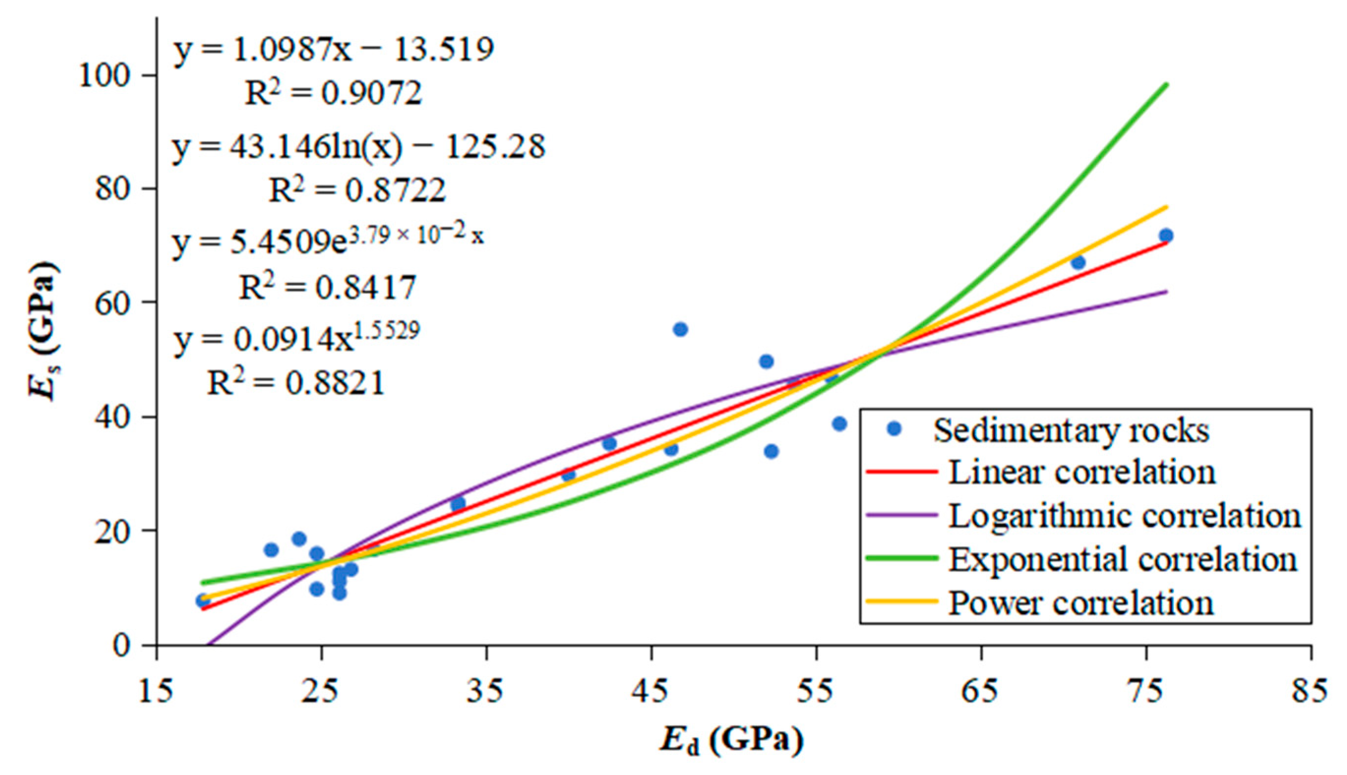
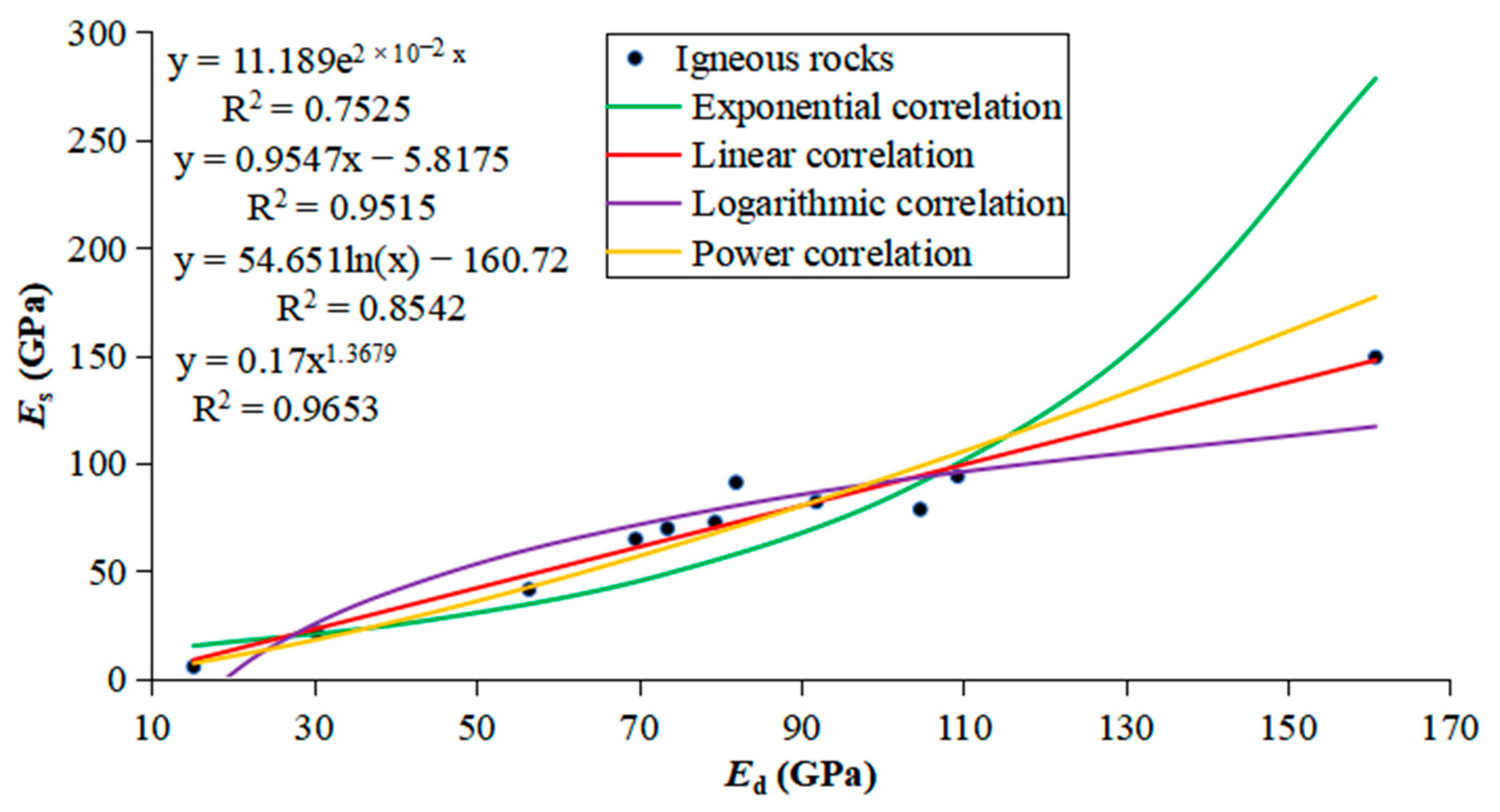
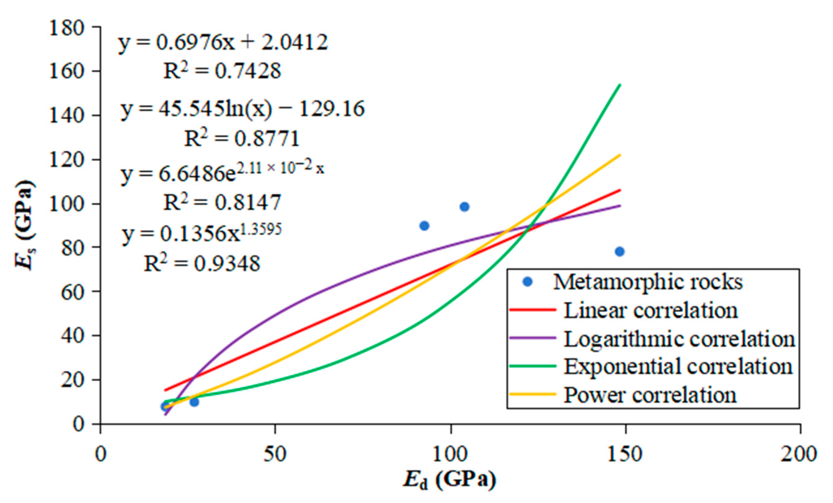
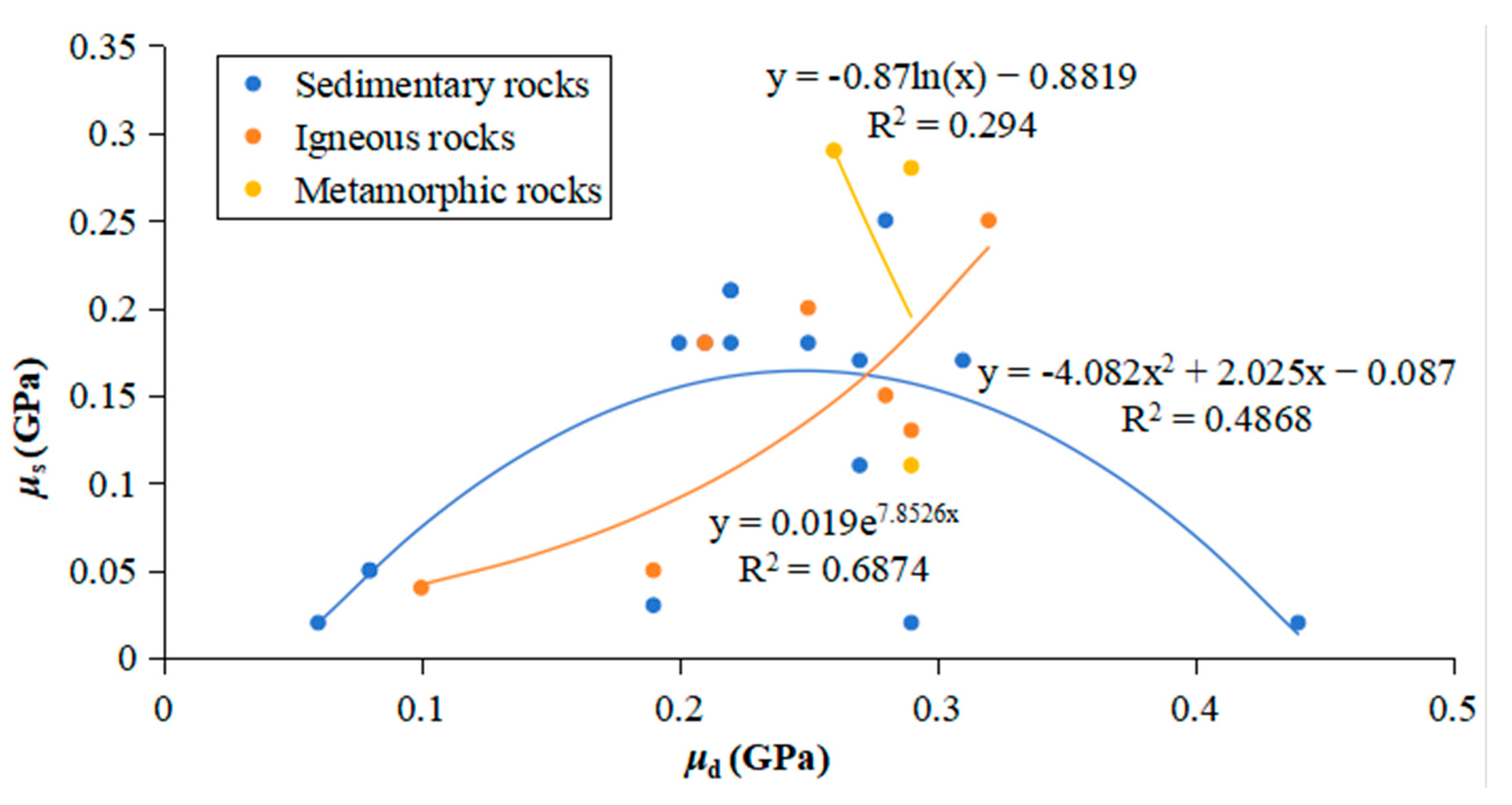
• Considering the correlation between static and dynamic moduli: In terms of different types of rocks, for igneous and metamorphic rocks, the optimal relationship between static and dynamic moduli of elasticity is a power-law correlation, with a value of (igneous R² = 0.97, metamorphic R² = 0.93), and for sedimentary rocks, a linear and nonlinear logarithmic correlation, with a value of (R² = 0.91).
• Predictive equations obtained by previous researchers may have errors in practical applications, some of which may be appropriate for specific rock types. Therefore, it is necessary to calibrate the constant values, and any calibration may imply new correlations.
• The discrepancy between the dynamic and static moduli of elasticity can be summarized as follows. The external factors include the amount of stress, strain amplitude, test confining pressure, test temperature, and the test frequency of the rock specimen. The internal factors are mainly the mineral composition, content, pore development degree, pore fluids, microfractures or microcracks, coupling between rock particles, cementation type and anisotropy of the rock, and so on. The existence of microfractures and pores in the rocks is the main reason for the differences.
• Many factors affect the mechanical properties of rocks, and the experimental results often show inevitable fluctuations. To obtain more representative results, research should be carried out based on the inclusion of a large number of empirical data for regression analysis.

Future research can focus on the following aspects:

Firstly, the reasons for the discrepancy between dynamic and static mechanical parameters are analyzed from the micro-mechanism of test conditions and rock structure characteristics, and then other methods to make up for the reasons for these differences, to accurately grasp the correlation between the dynamic and static elastic parameters.

Secondly, experiments should be conducted on the dynamic and static elastic parameters of rocks under reservoir circumstances. This is so because the validity of these relations is limited and local. So, in the future, it is possible to establish a faster, more accurate, and more efficient prediction model for obtaining static parameters without distinguishing rock types within an acceptable range of error, and then determine the conversion correlation between dynamic and static elastic parameters.

Finally, an excellent linear relationship exists between the dynamic and static moduli of elasticity, which can be directly fitted. However, the relationship between the dynamic and static Poisson’s ratios is more complex. In practice, it is necessary to consider parameters such as strain amplitude, test temperature, acoustic frequency, and porosity to improve the fitting relationship between the dynamic and static Poisson’s ratios. This provides a basis for evaluating formation compressibility and fracturing design schemes.

In summary, this review offers important references and insights to understand better the problems and challenges in dynamic and static elastic parameters. Based on the current research, new perspectives and future research directions have been proposed, with the hope that they may contribute to the development of our knowledge within this field.

References

1. Wang, J.; Xie, L.; Xie, H.; Li, C. Triaxial mechanical characteristics and constitutive model of oil sand in Fengcheng. J. Sichuan Univ. Eng. Sci. Ed. 2015, 47, 1–9. [Google Scholar]
2. Gao, Y.; Ren, Z.; Jiang, H.; Ding, S. A nonlinear elastic model for oil sands considering shear dilation and strain softening. Chin. J. Undergr. Space Eng. 2023, 19, 43–50. [Google Scholar]
3. Howarth, D.F. Apparatus to determine static and dynamic elastic moduli. Rock Mech. Rock Eng. 1984, 17, 255–264. [Google Scholar] [CrossRef]
4. Zisman, W.A. Comparison of the statically and seismologically determined elastic constants of rocks. Proc. Natl. Acad. Sci. USA 1933, 19, 680–686. [Google Scholar] [CrossRef]
5. Ide, J.M. Comparison of statically and dynamically determined Young’s modulus of rocks. Proc. Natl. Acad. Sci. USA 1936, 22, 81–92. [Google Scholar] [CrossRef] [PubMed]
6. Simmons, G.; Brace, W.F. Comparison of static and dynamic measurements of compressibility of rocks. J. Geophys. Res. 1965, 70, 5649–5656. [Google Scholar] [CrossRef]
7. King, M.S. Static and dynamic elastic properties of igneous and metamorphic rocks from the Canadian shield. Int. J. Rock Mech. Min. Sci. 1983, 20, 237–241. [Google Scholar] [CrossRef]
8. Savich, A.I. Generalized relations between static and dynamic indices of rock deformability. Hydrotech. Constr. 1984, 18, 394–400. [Google Scholar] [CrossRef]
9. Van Heerden, W.L. General relations between static and dynamic moduli of rocks. Int. J. Rock Mech. Min. Sci. Geomech. Abstr. Pergamon 1987, 24, 381–385. [Google Scholar] [CrossRef]
10. Eissa, E.A.; Kazi, A. Relation between static and dynamic Young’s moduli of rocks. Int. J. Rock Mech. Min. Geomech. Abstr. 1988, 25, 479–482. [Google Scholar] [CrossRef]
11. Wang, Z.; Nur, A. Dynamic versus static elastic properties of reservoir rocks. Seism. Acoust. Veloc. Reserv. Rocks 2000, 3, 531–539. [Google Scholar]
12. Al-Shayea, N.A. Effects of testing methods and conditions on the elastic properties of limestone rock. Eng. Geol. 2004, 74, 139–156. [Google Scholar] [CrossRef]
13. Kolesnikov, Y.I. Dispersion effect of velocities on the evaluation of material elasticity. J. Min. Sci. 2009, 45, 347–354. [Google Scholar] [CrossRef]
14. Aragón, G.; Pérez-Acebo, H.; Salas, M.Á.; Aragón-Torre, Á. Analysis f the static and dynamic elastic moduli of a one-coat rendering mortar with laboratory and in situ samples. Case Stud. Constr. Mater. 2024, 20, e02868. [Google Scholar] [CrossRef]
15. Ahrens, B.; Duda, M.; Renner, J. Relations between hydraulic properties and ultrasonic velocities during brittle failure of a low-porosity sandstone in laboratory experiments. Geophys. J. Int. 2018, 212, 627–645. [Google Scholar] [CrossRef]
16. Fjær, E. Relations between static and dynamic moduli of sedimentary rocks. Geophys. Prospect. 2019, 67, 128–139. [Google Scholar] [CrossRef]
17. Fjær, E. Static and dynamic moduli of a weak sandstone. Geophysics 2009, 74, WA103–WA112. [Google Scholar] [CrossRef]
18. Blake, O.O.; Faulkner, D.R.; Tatham, D.J. The role of fractures, effective pressure and loading on the difference between the static and dynamic Poisson’s ratio and Young’s modulus of Westerly granite. Int. J. Rock Mech. Min. Sci. 2019, 116, 87–98. [Google Scholar] [CrossRef]
19. Li, J.; Li, S. Calculation of Rock Mechanics Parameters Using Compressional and Shear Wave Data and Its Application. Well Logging Technol. 2003, (Suppl. S1), 15–18+87. [Google Scholar] [CrossRef]
20. Yale, D.P.; Jamieson, W.H. Static and Dynamic Rock Mechanical Properties in the Hugoton and Panoma Fields. In SPE Oklahoma City Oil and Gas Symposium/Production and Operations Symposium; SPE: Richardson, TX, USA, 1994; p. SPE-27939-MS. [Google Scholar]
21. Wang, H.; Liu, Y.; Dong, D.; Zhao, Q.; Du, D. Scientific issues on effective development of marine shale gas in southern China. Pet. Explor. Dev. 2013, 40, 615–620. [Google Scholar] [CrossRef]
22. Jia, C.; Chen, J.; Guo, Y.; Yang, C.; Xu, J.; Wang, L. Research on mechanical behaviors and failure modes of layer shale. Rock Soil Mech. 2013, 34 (Suppl. S2), 57–61. [Google Scholar]
23. Makoond, N.; Cabané, A.; Pelà, L.; Molins, C. Relationship between the static and dynamic elastic modulus of brick masonry constituents. Constr. Build. Mater. 2020, 259, 120386. [Google Scholar] [CrossRef]
24. Evans, W.M. A System for Combined Determination of Dynamic and Static Elastic Properties. In Permeability, Porosity and Resistivity of Rocks; The University of Texas: Austin, TX, USA, 1973. [Google Scholar]
25. Lama, R.D.; Vutukuri, V.S. Handbook on Mechanical Properties of Rocks: Testing Technique and Results; Trans Tech Publications: Clausthal-Zellerfeld, Germany, 1978. [Google Scholar]
26. Liao, J.J.; Hu, T.B.; Chang, C.W. Determination of dynamic elastic constants of transversely isotropic rocks using a single cylindrical specimen. Int. J. Rock Mech. Min. Sci. 1997, 34, 1045–1054. [Google Scholar] [CrossRef]
27. Warpinski, N.R.; Peterson, R.E.; Branagan, P.T.; Engler, B.P.; Wolhart, S.L. In situ stress and moduli: Comparison of values derived from multiple techniques. In Proceedings of the SPE Annual Technical Conference and Exhibition, New Orleans, LA, USA, 27–30 September 1998; p. SPE-49190. [Google Scholar]
28. Lin, Y.; Ge, H.; Wang, S. Testing Study on Dynamic and Static Elastic Parameters of Rcks. Chin. J. Rock Mech. Eng. 1998, 17, 216–222. [Google Scholar]
29. Belikov, B.P.; Alexandrov, K.S.; Rysova, T.W. Upruie Svoistva Porodoobrasujscich Mineralov I Gornich Porod; Izdat Nauka: Moskva, Russia, 1970. [Google Scholar]
30. McCann, D.M.; Entwisle, D.C. Determination of Young’s modulus of the rock mass from geophysical well logs. Geol. Soc. Spec. Pub. 1992, 65, 317–325. [Google Scholar] [CrossRef]
31. Canady, W. A method for full-range Young’s modulus correction. In Proceedings of the SPE Unconventional Resources Conference/Gas Technology Symposium, The Woodlands, TX, USA, 14–16 June 2011; p. SPE-143604. [Google Scholar]
32. Martínez-Martínez, J.; Benavente, D.; García-del-Cura, M.A. Comparison of the static and dynamic elastic modulus in carbonate rocks. Bull. Eng. Geol. Environ. 2012, 71, 263–268. [Google Scholar] [CrossRef]
33. Brotons, V.; Tomás, R.; Ivorra, S.; Grediaga, A.; Martínez-Martínez, J.; Benavente, D.; Gómez-Heras, M. Improved correlation between the static and dynamic elastic modulus of different types of rocks. Mater. Struct. 2016, 49, 3021–3037. [Google Scholar] [CrossRef]
34. Ciccotti, M.; Almagro, R.; Mulargia, F. Static and dynamic moduli of the seismogenic layer in Italy. Rock Mech. Rock Eng. 2004, 37, 229–238. [Google Scholar] [CrossRef]
35. Zhou, Y.; Gao, J.; Sun, Z.; Qu, W. A fundamental study on compressive strength, static and dynamic elastic moduli of young concrete. Constr. Build. Mater. 2015, 98, 137–145. [Google Scholar] [CrossRef]
36. Sun, Y.; Jing, W.; Ni, P.; Shen, W. Study on Dynamic and Static Elastic Modulus Transformation Relationship of Low Permeability Sandstone in CA Area. Oil Drill. Prod. Technol. 2022, 31, 15–18. [Google Scholar]
37. Ulusay, R.; Hudson, J.A. The Complete ISRM Suggested Methods for Rock Characterization, Testing and Monitoring; ISRM Turkish National Group: Ankara, Türkiye, 2007. [Google Scholar]
38. Han, S.H.; Kim, J.K. Effect of temperature and age on the relationship between dynamic and static elastic modulus of concrete. Cem. Concr. Res. 2004, 34, 1219–1227. [Google Scholar] [CrossRef]
39. Davarpanah, S.M.; Ván, P.; Vásárhelyi, B. Investigation of the relationship between dynamic and static deformation moduli of rocks. Geomech. Geophy. Geo-Energy Geo-Resour. 2020, 6, 29. [Google Scholar] [CrossRef]
40. Sun, F.; Yang, C.; Ma, S. An S-Wave Velocity Predicted Method. Prog. Geophys. 2008, 23, 470–474. [Google Scholar]
41. Shan, Y.; Liu, W. Experimental Study on Dynamic and Static Mechanics Parameters of Rocks under Formation Conditions. J. Chengdu Univ. Technol. Sci. Technol. Ed. 2000, 27, 249–254. [Google Scholar]
42. Gao, Y.; Chen, M.; Pang, H. Experimental investigations on elastoplastic deformation and permeability evolution of terrestrial Karamay oil sands at high temperatures and pressures. J. Pet. Sci. Eng. 2020, 190, 107124. [Google Scholar] [CrossRef]
43. Christaras, B.; Auger, F.; Mosse, E. Determination of the moduli of elasticity of rocks. Comparison of the ultrasonic velocity and mechanical resonance frequency methods with direct static methods. Mater. Struct. 1994, 27, 222–228. [Google Scholar] [CrossRef]
44. Neville, A.M. Properties of Concrete; Longman: London, UK, 1995; Volume 4. [Google Scholar]
45. CP110, Code of Practice for the Structural Use of Concrete; British Standards Institution: London, UK, 1972.
46. Lacy, L.L. Dynamic rock mechanics testing for optimized fracture designs. In Proceedings of the SPE Annual Technical Conference and Exhibition, San Antonio, TX, USA, 5–8 October 1997. [Google Scholar]
47. Brautigam, T.; Knochel, A.; Lehne, M. Prognosis of uniaxial compressive strength and stiffness of rocks based on point load and ultrasonic tests. Otto-Graf-J 1998, 9, 61–79. [Google Scholar]
48. Nur, A.; Wang, Z. Seismic and Acoustic Velocities in Reservoir Rocks: Recent Developments; Society of Exploration Geophysicists: Tulsa, OK, USA, 1999. [Google Scholar]
49. Helvatjoglu-Antoniades, M.; Papadogiannis, Y.; Lakes, R.S.; Dionysopoulos, P.; Papadogiannis, D. Dynamic and static elastic moduli of packable and flowable composite resins and their development after initial photo curing. Dent. Mater. 2006, 22, 450–459. [Google Scholar] [CrossRef]
50. Mockovčiaková, A.; Pandula, B. Study of the relation between the static and dynamic moduli of rocks. Metalurgija 2003, 42, 37–39. [Google Scholar]
51. Fahimifar, A.; Soroush, H. Evaluation of Some Physical and Mechanical Properties of Rocks Using Ultrasonic Pulse Technique and Presenting Equations between Dynamic and Static Elastic Constants. In ISRM Congress; South African Institute of Mining and Etallurgy–Technology Roadmap for Rock Mechanics, ISRM: Lisbon, Portugal, 2003. [Google Scholar]
52. Al-Tahini, A.M. The Effect of Cementation on the Mechanical Properties for Jauf Reservoir at Saudi Arabia. Ph.D. Thesis, University of Oklahoma, Norman, OK, USA, 2003. [Google Scholar]
53. Ohen, H.A. Calibrated Wireline Mechanical Rock Properties Method for Predicting and Preventing Wellbore Collapse and Sanding. In Proceedings of the SPE European Formation Damage Conference and Exhibition, The Hague, The Netherlands, 13–14 May 2003; p. SPE-82236. [Google Scholar]
54. Ameen, M.S.; Smart, B.G.; Somerville, J.M.; Hammilton, S.; Naji, N.A. Predicting rock mechanical properties of carbonates from wireline logs (A ase study: Arab-D reservoir, Ghawar field, Saudi Arabia). Mar. Pet. Geol. 2009, 26, 430–444. [Google Scholar] [CrossRef]
55. Brotons, V.; Tomás, R.; Ivorra, S.; Grediaga, A. Relationship between static and dynamic elastic modulus of calcarenite heated at different temperatures: The San Julián’s stone. Bull. Eng. Geol. Environ. 2014, 73, 791–799. [Google Scholar] [CrossRef]
56. Najibi, A.R.; Ghafoori, M.; Lashkaripour, G.R.; Asef, M.R. Empirical relations between strength and static and dynamic elastic properties of Asmari and Sarvak limestones, two main oil reservoirs in Iran. J. Pet. Sci. Eng. 2015, 126, 78–82. [Google Scholar] [CrossRef]
57. Horsrud, P. Estimating mechanical properties of shale from empirical correlations. SPE Drill. Complet. 2001, 16, 68–73. [Google Scholar] [CrossRef]
58. Asef, M.R.; Farrokhrouz, M. A semi-empirical relation between static and dynamic elastic modulus. J. Pet. Sci. Eng. 2017, 157, 359–363. [Google Scholar] [CrossRef]
59. Tutuncu, A.N.; Podio, A.L.; Gregory, A.R.; Sharma, M.M. Nonlinear viscoelastic behavior of sedimentary rocks, Part I: Effect of frequency and strain amplitude. Geophysics 1998, 63, 184–194. [Google Scholar] [CrossRef]
60. Gong, F.; Di, B.; Wei, J.; Ding, P.; Tian, H.; Han, J. A study of the anisotropic static and dynamic elastic properties of transversely isotropic rocks. Geophysics 2019, 84, C281–C293. [Google Scholar] [CrossRef]
61. Zhang, L.; Ba, J.; Fu, L.; Carcione, J.M.; Cao, C. Estimation of pore microstructure by using the static and dynamic moduli. Int. J. Rock Mech. Min. Sci. 2019, 113, 24–30. [Google Scholar] [CrossRef]
62. Fei, W.; Huiyuan, B.; Jun, Y.; Yonghao, Z. Correlation of dynamic and static elastic parameters of rock. Electron. J. Geotech. Eng. 2016, 21, 1551–1560. [Google Scholar]
63. Bakhorji, A.; Schmitt, D.R. Laboratory measurements of static and dynamic bulk moduli in carbonate. In ARMA US Rock Mechanics/Geomechanics Symposium; ARMA: Alexandria, VA, USA, 2010; p. ARMA-10. [Google Scholar]
64. Blake, O.O.; Faulkner, D.R. The effect of fracture density and stress state on the static and dynamic bulk moduli of Westerly granite. J. Geophys. Res. Solid Earth 2016, 121, 2382–2399. [Google Scholar] [CrossRef]
Figure 1. (a) is the tangent elastic modulus, (b) is the average elastic modulus, (c) is the secant elastic modulus [39].
Applsci 14 04487 g001
Figure 2. Experiment schematic diagram.
Applsci 14 04487 g002
Figure 4. Relationship between Ed and Es in the studied specimens. The straight line corresponds to the ideal ratio Ed/Es = 1 [32].
Applsci 14 04487 g004
Figure 5. Correlation between a and b constants [39].
Applsci 14 04487 g005
Figure 6. Correlation between a and b constants.
Applsci 14 04487 g006
Figure 7. Correlation between static (Es) and dynamic (Ed) moduli proposed by various authors [7,10,29,30,32,33,43,44,45,46,47,48,49,51,53,54,55,56].
Applsci 14 04487 g007
Figure 8. Relationship between different curves fits for the dynamic and static elastic moduli of sedimentary rocks.
Applsci 14 04487 g008
Figure 9. Relationship between different curve fits of dynamic and static elastic moduli of igneous rocks.
Applsci 14 04487 g009
Figure 10. Relationship between different curve fits of dynamic and static elastic moduli of metamorphic rocks.
Applsci 14 04487 g010
Figure 11. Log–coordinate fitting relationship for dynamic and static elastic moduli of sedimentary rocks.
Applsci 14 04487 g011
Figure 12. Dynamic and static elastic moduli log–coordinate fitting relationships for igneous rocks.
Applsci 14 04487 g012
Figure 13. Dynamic and static elastic moduli log–coordinate fitting relationships for metamorphic rocks.
Applsci 14 04487 g013
Figure 14. R2 for linear correlation, power-law correlation, and nonlinear logarithmic correlation between static and dynamic for various rock types.
Applsci 14 04487 g014
Figure 15. Dynamic and static Poisson’s ratio fitting relationships for different types of rocks.
Applsci 14 04487 g015