
Time–Frequency Domain Seismic Signal Denoising Based on Generative Adversarial Networks


Abstract
1. Introduction
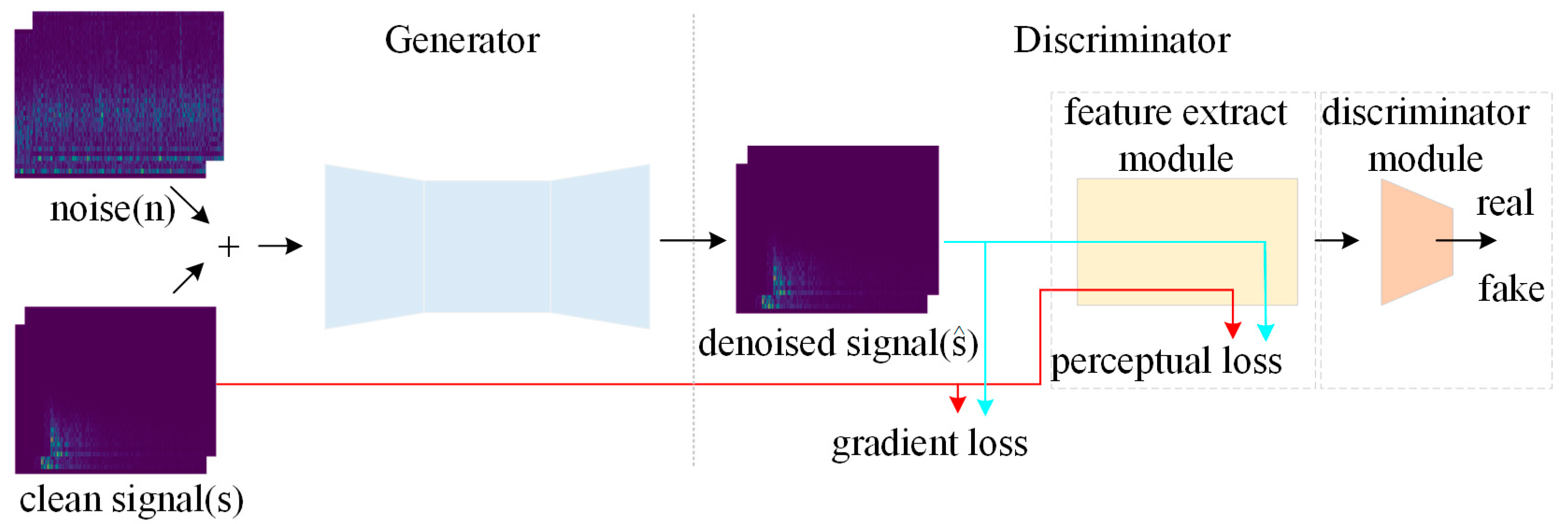
2. Method
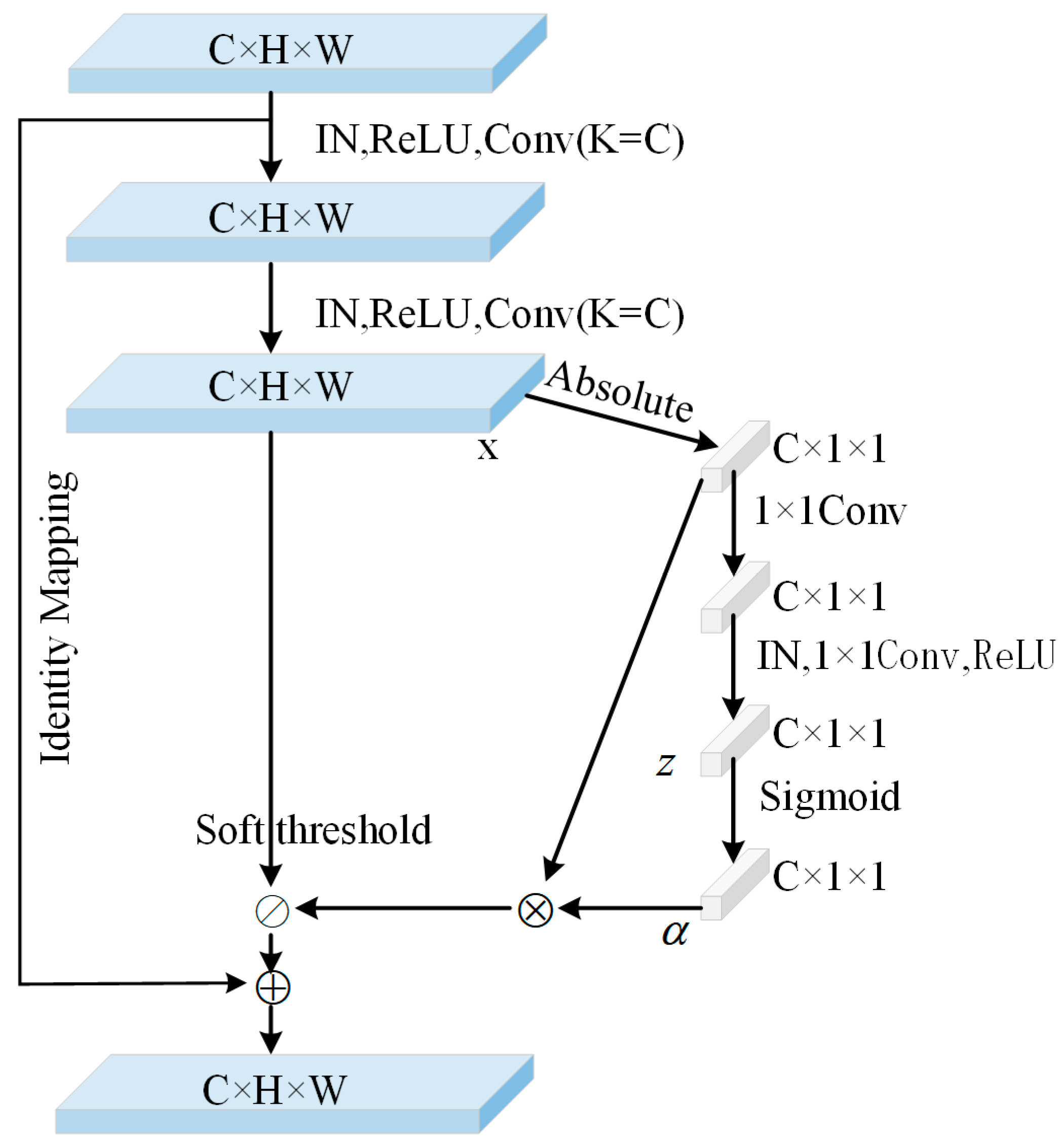
2.1. Generator Network Structure
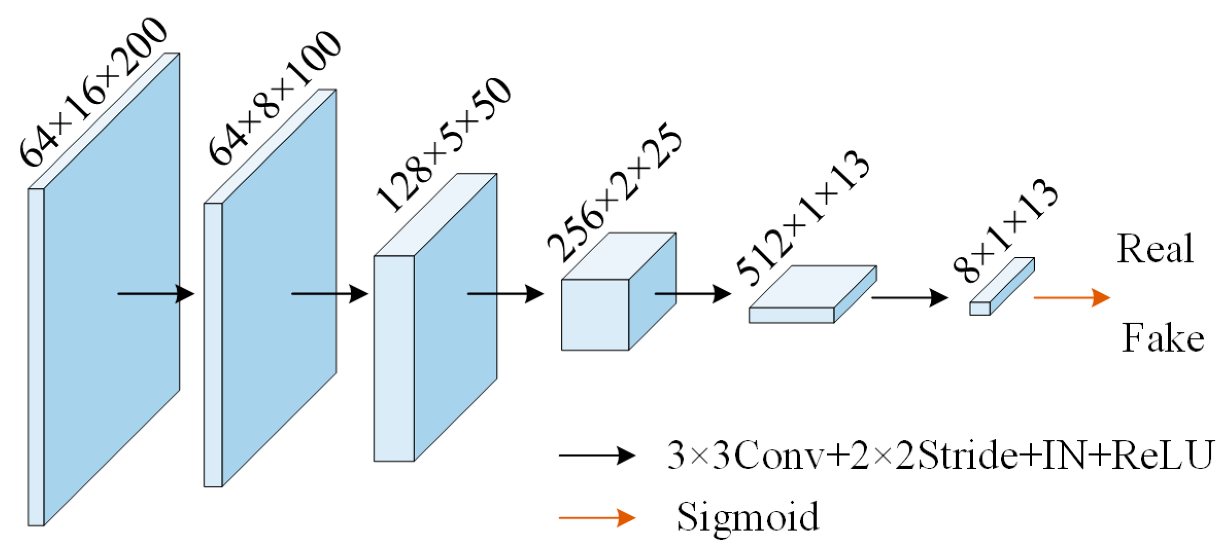
2.2. Discriminator Network Structure
2.3. Loss Function
3. Results
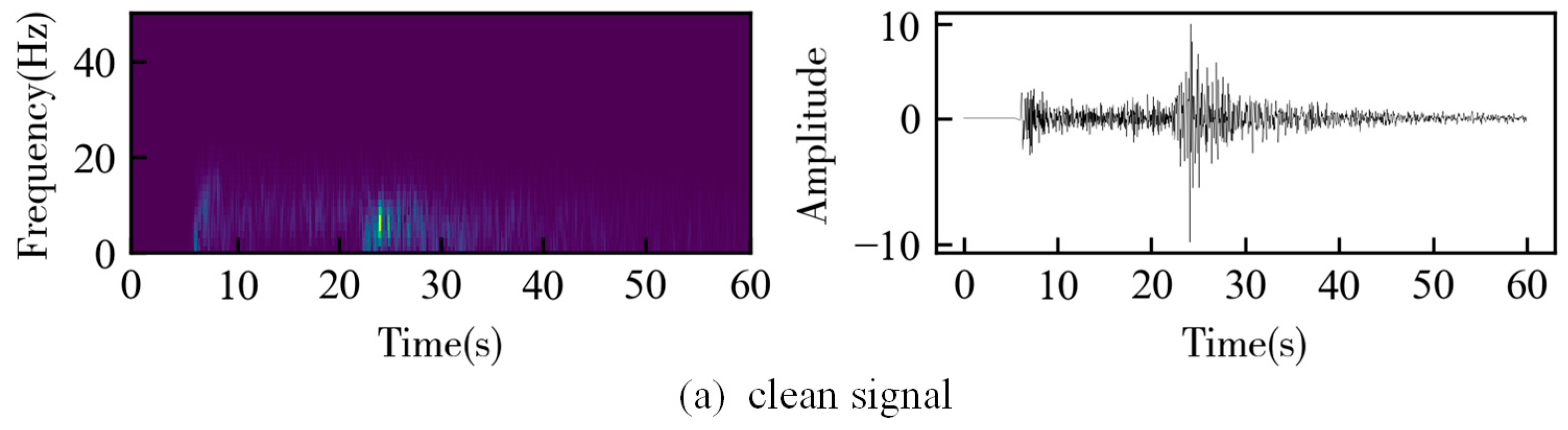
3.1. Synthetic Data
3.2. Field Data
4. Discussion
Author Contributions
Funding
Institutional Review Board Statement
Informed Consent Statement
Data Availability Statement
Conflicts of Interest
References
- Brett, H.; Hawkins, R.; Waszek, L.; Lythgoe, K.; Deuss, A. 3D Transdimensional Seismic Tomography of the Inner Core. Earth Planet. Sci. Lett. 2022, 593, 117688. [Google Scholar] [CrossRef]
- Tassiopoulou, S.; Koukiou, G.; Anastassopoulos, V. Algorithms in Tomography and Related Inverse Problems—A Review. Algorithms 2024, 17, 71. [Google Scholar] [CrossRef]
- Zhang, J.; Shi, M.; Wang, D.; Tong, Z.; Hou, X.; Niu, J.; Li, X.; Li, Z.; Zhang, P.; Huang, Y. Fields and Directions for Shale Gas Exploration in China. Nat. Gas Ind. B 2022, 9, 20–32. [Google Scholar] [CrossRef]
- Wang, W.; Xue, C.; Zhao, J.; Yuan, C.; Tang, J. Machine Learning-Based Field Geological Mapping: A New Exploration of Geological Survey Data Acquisition Strategy. Ore Geol. Rev. 2024, 166, 105959. [Google Scholar] [CrossRef]
- da Silva, S.L.; Costa, F.; Karsou, A.; Capuzzo, F.; Moreira, R.; Lopez, J.; Cetale, M. Research Note: Application of Refraction Full-Waveform Inversion of Ocean Bottom Node Data Using a Squared-Slowness Model Parameterization. Geophys. Prospect. 2024, 72, 1189–1195. [Google Scholar] [CrossRef]
- Fehler, M.C.; Huang, L. Modern Imaging Using Seismic Reflection Data. Annu. Rev. Earth Planet. Sci. 2002, 30, 259–284. [Google Scholar] [CrossRef]
- Wang, F.; Yang, B.; Wang, Y.; Wang, M. Learning From Noisy Data: An Unsupervised Random Denoising Method for Seismic Data Using Model-Based Deep Learning. IEEE Trans. Geosci. Remote Sens. 2022, 60, 1–14. [Google Scholar] [CrossRef]
- Cao, S.; Chen, X. The Second-Generation Wavelet Transform and Its Application in Denoising of Seismic Data. Appl. Geophys. 2005, 2, 70–74. [Google Scholar] [CrossRef]
- Chen, X.; He, Z. Improved S-Transform and Its Application in Seismic Signal Processing. Available online: https://www.researchgate.net/publication/298264611_Improved_S-transform_and_its_application_in_seismic_signal_processing (accessed on 15 March 2024).
- Jicheng, L.; Gu, Y.; Chou, Y.; Gu, J. Seismic Data Random Noise Reduction Using a Method Based on Improved Complementary Ensemble EMD and Adaptive Interval Threshold. Explor. Geophys. 2021, 52, 137–149. [Google Scholar] [CrossRef]
- Li, W.; Liu, H.; Wang, J. A Deep Learning Method for Denoising Based on a Fast and Flexible Convolutional Neural Network. IEEE Trans. Geosci. Remote Sens. 2022, 60, 1–13. [Google Scholar] [CrossRef]
- Zhong, T.; Cheng, M.; Dong, X.; Wu, N. Seismic Random Noise Attenuation by Applying Multiscale Denoising Convolutional Neural Network. IEEE Trans. Geosci. Remote Sens. 2022, 60, 1–13. [Google Scholar] [CrossRef]
- Zhao, H.; Zhou, Y.; Bai, T.; Chen, Y. A U-Net Based Multi-Scale Deformable Convolution Network for Seismic Random Noise Suppression-All Databases. Available online: https://webofscience.clarivate.cn/wos/alldb/full-record/WOS:001072548400001 (accessed on 3 February 2024).
- Lan, T.; Han, L.; Zeng, Z.; Zeng, J. An Attention-Based Residual Neural Network for Efficient Noise Suppression in Signal Processing. Appl. Sci. 2023, 13, 5262. [Google Scholar] [CrossRef]
- Zhu, W.; Mousavi, S.M.; Beroza, G.C. Seismic Signal Denoising and Decomposition Using Deep Neural Networks. IEEE Trans. Geosci. Remote Sens. 2019, 57, 9476–9488. [Google Scholar] [CrossRef]
- Gao, Z.; Zhang, S.; Cai, J.; Hong, L.; Zheng, J. Research on Deep Convolutional Neural Network Time-Frequency Domain Seismic Signal Denoising Combined with Residual Dense Blocks. Front. Earth Sci. 2021, 9, 681869. [Google Scholar] [CrossRef]
- Cai, J.; Wang, L.; Zheng, J.; Duan, Z.; Li, L.; Chen, N. Denoising Method for Seismic Co-Band Noise Based on a U-Net Network Combined with a Residual Dense Block. Appl. Sci. 2023, 13, 1324. [Google Scholar] [CrossRef]
- Donoho, D.L.; Johnstone, I.M. Ideal Spatial Adaptation by Wavelet Shrinkage. Biometrika 1994, 81, 425–455. [Google Scholar] [CrossRef]
- Li, Y.; Wang, N.; Shi, J.; Liu, J.; Hou, X. Revisiting Batch Normalization For Practical Domain Adaptation. arXiv 2019, arXiv:1603.04779. [Google Scholar]
- Singh, A.; Hingane, S.; Gong, X.; Wang, Z. SAFIN: Arbitrary Style Transfer with Self-Attentive Factorized Instance Normalization. In Proceedings of the 2021 IEEE International Conference on Multimedia and Expo (ICME), Shenzhen, China, 5 July 2021; IEEE: New York, NY, USA, 2021; pp. 1–6. [Google Scholar]
- Huang, L.; Qin, J.; Zhou, Y.; Zhu, F.; Liu, L.; Shao, L. Normalization Techniques in Training DNNs: Methodology, Analysis and Application. IEEE Trans. Pattern Anal. Mach. Intell. 2023, 45, 10173–10196. [Google Scholar] [CrossRef] [PubMed]
- Shi, Y.; Huang, Z.; Huang, Z.; Hua, X.; Hong, H.; Li, L. HINRDNet: A Half Instance Normalization Residual Dense Network for Passive Millimetre Wave Image Restoration. Infrared Phys. Technol. 2023, 132, 104722. [Google Scholar] [CrossRef]
- Tarasiewicz, T.; Nalepa, J.; Farrugia, R.A.; Valentino, G.; Chen, M.; Briffa, J.A.; Kawulok, M. Multitemporal and Multispectral Data Fusion for Super-Resolution of Sentinel-2 Images. IEEE Trans. Geosci. Remote Sens. 2023, 61, 1–19. [Google Scholar] [CrossRef]
- Chen, L.; Lu, X.; Zhang, J.; Chu, X.; Chen, C. HINet: Half Instance Normalization Network for Image Restoration. In Proceedings of the 2021 IEEE/CVF Conference on Computer Vision and Pattern Recognition Workshops (CVPRW), Nashville, TN, USA, 19–25 June 2021; IEEE: New York, NY, USA, 2021; pp. 182–192. [Google Scholar]
- Springenberg, J.T.; Dosovitskiy, A.; Brox, T.; Riedmiller, M. Striving for Simplicity: The All Convolutional Net. arXiv 2019, arXiv:1412.6806. [Google Scholar]
- Odena, A.; Dumoulin, V.; Olah, C. Deconvolution and Checkerboard Artifacts. Distill 2016, 1, e3. [Google Scholar] [CrossRef]
- He, K.; Zhang, X.; Ren, S.; Sun, J. Deep Residual Learning for Image Recognition. In Proceedings of the 2016 IEEE Conference on Computer Vision and Pattern Recognition (CVPR), Las Vegas, NV, USA, 27–30 June 2016; IEEE: New York, NY, USA, 2016; pp. 770–778. [Google Scholar]
- Zhao, M.; Zhong, S.; Fu, X.; Tang, B.; Pecht, M. Deep Residual Shrinkage Networks for Fault Diagnosis. IEEE Trans. Ind. Inform. 2020, 16, 4681–4690. [Google Scholar] [CrossRef]
- Lin, L.; Zhong, Z.; Li, C. SeisGAN: Improving Seismic Image Resolution and Reducing Random Noise Using a Generative Adversarial Network | Mathematical Geosciences. Available online: https://link.springer.com/article/10.1007/s11004-023-10103-8 (accessed on 13 December 2023).
- Li, Y.; Wang, S.; Jiang, M. Seismic Random Noise Suppression by Using MSRD-GAN. Geoenergy Sci. Eng. 2023, 222, 211410. [Google Scholar] [CrossRef]
- Simonyan, K.; Zisserman, A. Very Deep Convolutional Networks for Large-Scale Image Recognition. arXiv 2015, arXiv:1409.1556. [Google Scholar]
- Russakovsky, O.; Deng, J.; Su, H.; Krause, J.; Satheesh, S.; Ma, S.; Huang, Z.; Karpathy, A.; Khosla, A.; Bernstein, M.; et al. ImageNet Large Scale Visual Recognition Challenge. Int. J. Comput. Vis. 2015, 115, 211–252. [Google Scholar] [CrossRef]
- Shi, W.; Caballero, J.; Huszar, F.; Totz, J.; Aitken, A.P.; Bishop, R.; Rueckert, D.; Wang, Z. Real-Time Single Image and Video Super-Resolution Using an Efficient Sub-Pixel Convolutional Neural Network. In Proceedings of the 2016 IEEE Conference on Computer Vision and Pattern Recognition (CVPR), Las Vegas, NV, USA, 27–30 June 2016; IEEE: New York, NY, USA, 2016; pp. 1874–1883. [Google Scholar]
- Woo, S.; Park, J.; Lee, J.-Y.; Kweon, I.S. CBAM: Convolutional Block Attention Module. In Computer Vision—ECCV 2018; Ferrari, V., Hebert, M., Sminchisescu, C., Weiss, Y., Eds.; Lecture Notes in Computer Science; Springer International Publishing: Cham, Switzerland, 2018; Volume 11211, pp. 3–19. ISBN 978-3-030-01233-5. [Google Scholar]
- Canny, J. A Computational Approach to Edge Detection. IEEE Trans. Pattern Anal. Mach. Intell. 1986, PAMI-8, 679–698. [Google Scholar] [CrossRef]
- Ma, C.; Rao, Y.; Cheng, Y.; Chen, C.; Lu, J.; Zhou, J. Structure-Preserving Super Resolution with Gradient Guidance. In Proceedings of the IEEE/CVF Conference on Computer Vision and Pattern Recognition (CVPR) 2020, Seattle, WA, USA, 13–19 June 2020; pp. 7769–7778. [Google Scholar]
- Furnari, A.; Farinella, G.M.; Bruna, A.R.; Battiato, S. Generalized Sobel Filters for Gradient Estimation of Distorted Images. In Proceedings of the 2015 IEEE International Conference on Image Processing (ICIP), Quebec City, QC, Canada, 27–30 September 2015; pp. 3250–3254. [Google Scholar]
- Mousavi, S.M.; Sheng, Y.; Zhu, W.; Beroza, G.C. STanford EArthquake Dataset (STEAD): A Global Data Set of Seismic Signals for AI. IEEE Access 2019, 7, 179464–179476. [Google Scholar] [CrossRef]


| Signal SNR (dB) | DeepDenoiser | ARDU | Ours |
|---|---|---|---|
| −1 | 2.568 | 4.933 | 6.945 |
| 0 | 4.086 | 7.593 | 9.384 |
| 1 | 10.802 | 11.650 | 14.471 |
| 2 | 12.643 | 13.001 | 14.229 |
| 3 | 14.847 | 15.480 | 15.502 |
| 4 | 19.111 | 20.444 | 16.081 |
| 5 | 21.425 | 21.065 | 16.021 |
| 6 | 21.934 | 22.351 | 15.857 |
| 7 | 23.350 | 23.015 | 16.173 |
| Signal SNR (dB) | DeepDenoiser | ARDU | Ours |
|---|---|---|---|
| −1 | 0.387 | 0.391 | 0.499 |
| 0 | 0.453 | 0.466 | 0.558 |
| 1 | 0.703 | 0.709 | 0.772 |
| 2 | 0.793 | 0.797 | 0.841 |
| 3 | 0.870 | 0.873 | 0.914 |
| 4 | 0.910 | 0.910 | 0.954 |
| 5 | 0.932 | 0.935 | 0.978 |
| 6 | 0.938 | 0.957 | 0.976 |
| 7 | 0.942 | 0.960 | 0.974 |
| Signal SNR (dB) | DeepDenoiser | ARDU | Ours |
|---|---|---|---|
| −1 | 0.249 | 0.242 | 0.239 |
| 0 | 0.248 | 0.242 | 0.237 |
| 1 | 0.197 | 0.194 | 0.187 |
| 2 | 0.185 | 0.161 | 0.163 |
| 3 | 0.170 | 0.147 | 0.132 |
| 4 | 0.151 | 0.126 | 0.109 |
| 5 | 0.139 | 0.115 | 0.096 |
| 6 | 0.147 | 0.119 | 0.096 |
| 7 | 0.147 | 0.111 | 0.098 |
| Method | Floating-Point Operations (G) | Number of Parameters (M) |
|---|---|---|
| DeepDenoiser | 0.31 | 2.65 |
| ARDU | 6.83 | 40.87 |
| Ours | 6.67 | 17.27 |
Disclaimer/Publisher’s Note: The statements, opinions and data contained in all publications are solely those of the individual author(s) and contributor(s) and not of MDPI and/or the editor(s). MDPI and/or the editor(s) disclaim responsibility for any injury to people or property resulting from any ideas, methods, instructions or products referred to in the content. |
© 2024 by the authors. Licensee MDPI, Basel, Switzerland. This article is an open access article distributed under the terms and conditions of the Creative Commons Attribution (CC BY) license (https://creativecommons.org/licenses/by/4.0/).
Share and Cite
Wei, M.; Sun, X.; Zong, J. Time–Frequency Domain Seismic Signal Denoising Based on Generative Adversarial Networks. Appl. Sci. 2024, 14, 4496. https://doi.org/10.3390/app14114496
Wei M, Sun X, Zong J. Time–Frequency Domain Seismic Signal Denoising Based on Generative Adversarial Networks. Applied Sciences. 2024; 14(11):4496. https://doi.org/10.3390/app14114496
Chicago/Turabian StyleWei, Ming, Xinlei Sun, and Jianye Zong. 2024. "Time–Frequency Domain Seismic Signal Denoising Based on Generative Adversarial Networks" Applied Sciences 14, no. 11: 4496. https://doi.org/10.3390/app14114496
APA StyleWei, M., Sun, X., & Zong, J. (2024). Time–Frequency Domain Seismic Signal Denoising Based on Generative Adversarial Networks. Applied Sciences, 14(11), 4496. https://doi.org/10.3390/app14114496