Abstract
For system identification problems associated with long-length impulse responses, the recently developed decomposition-based technique that relies on a third-order tensor (TOT) framework represents a reliable choice. It is based on a combination of three shorter filters, which merge their estimates in tandem with the Kronecker product. In this way, the global impulse response is modeled in a more efficient manner, with a significantly reduced parameter space (i.e., fewer coefficients). In this paper, we further develop a Kalman filter based on the TOT decomposition method. As compared to the recently designed recursive least-squares (RLS) counterpart, the proposed Kalman filter achieves superior performance in terms of the main criteria (e.g., tracking and accuracy). In addition, it significantly outperforms the conventional Kalman filter, while also having a lower computational complexity. Simulation results obtained in the context of echo cancellation support the theoretical framework and the related advantages.
1. Introduction
The Kalman filter is recognized as a popular signal processing tool in the framework of many real-world applications [1,2,3]. Among them, it has successfully been used in echo cancellation scenarios [4,5,6,7,8,9], aiming to model an unknown impulse response corresponding to the echo path. Nevertheless, the finite impulse response filter associated with this impulse response is usually characterized by a very large number of coefficients, which reaches the order of hundreds or even thousands. Such a large parameter space significantly impacts the overall performance of the Kalman filter, especially in terms of the convergence behavior, solution accuracy, and computational complexity.
In system identification problems like echo cancellation it is always helpful to exploit the particular characteristics of the impulse responses to be estimated. For example, echo paths are sparse in nature, i.e., only a small number of coefficients (as compared to the full length of the impulse response) have a significant magnitude, while the rest of them are close to zero or even null. The adaptive algorithms that take advantage of this feature are designed based on a “proportionate” approach [10], in which the significant coefficients are emphasized during the updating process. Due to this technique, the resulting proportionate-type adaptive filters achieve higher converge rates as compared to their conventional counterparts. Following the proportionate normalized least-mean-squares (PNLMS) algorithm from [10], different related versions were developed, like the mu-law PNLMS [11], the sparseness-controlled PNLMS [12], the PNLMS with individual activation factors [13], or the block-sparse PNLMS [14]. Also, the sparseness features were exploited in the framework of other categories of adaptive filtering algorithms, like the sign affine projection algorithm [15], recursive least-squares (RLS) algorithms with penalties [16,17], nonlinear filtering architectures [18], and subband adaptive filters [19,20]. In addition to echo cancellation, these sparsity-aware filters have been applied in the context of a wide range of applications, including underwater acoustics [21,22], channel estimation [23], and system identification [24]. A connection between the Kalman filter and several proportionate-type algorithms was established in [7]. Nevertheless, all these proportionate adaptive filters still involve the full length of the impulse response, so they face the related difficulties associated with a large number of coefficients.
In this context, a useful technique to reduce the parameter space takes advantage of the low-rank characteristic of the impulse responses, which fits very well for the estimation of echo path models [25]. In other words, the corresponding matrices associated with the reshaped impulse responses of the echo paths are never full-rank. This can be further exploited based on the nearest Kronecker product (NKP) decomposition, so that the adaptive filter estimate results based on a combination of shorter impulse responses, thus involving a smaller number of coefficients. In this decomposition framework, the NKP-based technique was applied to the RLS algorithm [26], the Kalman filter [27], the normalized least-mean-squares (NLMS) algorithm [28], correntropy-based methods [29], and nonlinear adaptive filters [30,31,32]. Related applications include acoustic feedback cancellation [33], adaptive beamforming [34], and acoustic echo cancellation [35], among others.
Following the NKP-based approach, the decomposition technique has been recently applied in conjunction with higher-order tensors [36,37], thus leading to higher-dimensionality reduction. It is known that tensor-based signal processing [38,39,40] represents an important asset in the framework of many applications, like big data analysis [41], biomedical engineering [42], blind source separation [43], and machine learning [44]. As a result, in long-length system identification scenarios, the RLS adaptive filter using a third-order tensor (TOT) decomposition from [37] outperforms its previously developed NKP-based counterpart designed in [26]. There is a well-established relation between the RLS algorithm and the Kalman filter, as supported in [2]. While there is a (misleading) resemblance between the two algorithms, the Kalman filter allows for better control in time-varying environments [7]. Nevertheless, due to the specific features of the TOT decomposition, there is not a straightforward extension from the RLS-TOT [37] towards the corresponding Kalman filter.
In this paper, motivated by the previous aspects and expected performance gain, we design a Kalman filter based on TOT decomposition. The main goals of our proposal target three basic directions. First, we aim to show that the developed Kalman filter based on TOT decomposition outperforms the conventional Kalman filter, in terms of both performance and complexity. Second, with the proposed TOT-based solution, we target a better performance as compared to the previously developed NKP-based version from [27], which exploits a second-order decomposition level. Third, the goal is to outperform the recently introduced RLS-TOT algorithm from [37], which applies the TOT decomposition in the framework of the RLS filter.
In order to develop our proposal, the rest of the manuscript is organized as follows. Section 2 presents the necessary background concerning the system identification scenario, the conventional Kalman filter, and the TOT decomposition framework. Then, the proposed Kalman filter based on TOT is developed in Section 3. Simulation results are provided in Section 4, using echo cancellation as the experimental setup. Finally, conclusions and future works are summarized in Section 5.
2. System Identification and TOT Decomposition
This section reviews the required background for the upcoming developments. First, the system identification scenario is presented, followed by the solution based on the conventional Kalman filter. Finally, the TOT decomposition of the impulse response is summarized.
2.1. System Identification Framework
The system identification framework addressed in this paper considers a linear single-input single-output (SISO) scenario with zero-mean real-valued signals, where the main goal is to identify an unknown system characterized by the impulse response of length L, where n is the discrete-time index and superscript denotes transposition. Also, let us consider that this time-varying impulse response evolves based on a simplified first-order Markov model, i.e.,
where is a vector of length L, which contains the samples of a zero-mean white Gaussian noise. In this context, and are uncorrelated. This standard model has been extensively involved in many analyses of time-varying systems in the framework of adaptive filtering algorithms [45,46,47]. In addition, it fits very well in echo cancellation scenarios [48]. Since is white and Gaussian, its covariance matrix is a diagonal one, which can be expressed as , where is the noise variance and denotes the identity matrix of size . It can be noticed that the uncertainties in are captured by .
2.2. Conventional Kalman Filter
In the context of Kalman filtering, the model from (1) represents the so-called state equation. In this framework, the observation equation is defined as the output of the system, related to the reference (or desired) signal, . It contains the convolution product between the samples of the input signal, , and the coefficients of the impulse response, , and is corrupted by an additive noise, . It is considered that this noise is white and Gaussian, with variance , where represents mathematical expectation. Consequently,
where the vector contains the L most recent time samples of the input signal. Next, considering an estimate of the impulse response at time index n, denoted by , the a priori estimation error results in
while the a posteriori error is defined as
Related to these estimates, we can also define the a priori and a posteriori misalignments, i.e.,
which are also known as the system mismatches [48] or state estimation errors. Based on (1), it can be easily checked that . Also, using (3) and (4), we have .
At this point, the Kalman filter can be obtained based on the linear sequential Bayesian approach, which states that the optimal estimate of the state vector is [49]
where is the Kalman gain vector [1]. This results by minimizing the cost function
where represents the trace of a square matrix and is the covariance matrix of the a posteriori misalignment from (6). From this optimization criterion, as shown in [49], two important results are obtained, as follows:
where is the covariance matrix of the a priori misalignment from (5), with
The initialization of the Kalman filter is and , where denotes an all-zeros vector of length L and is a positive constant. Then, in each iteration, the algorithm starts by computing the a priori error from (3) and evaluating the matrix from (11). Next, the Kalman gain vector and the matrix are computed using (9) and (10), respectively. Finally, the filter is updated based on (7). The specific parameters and can be a priori provided or estimated within the algorithm, as indicated in [7].
2.3. TOT Decomposition
The computational complexity of the conventional Kalman filter is proportional to the square of the filter length, i.e., . This represents a significant challenge when dealing with the identification of long-length impulse responses, which is usually the case in echo cancellation scenarios. In addition, other important performance criteria are also influenced by the length of the filter, like the convergence rate and tracking capability, together with the accuracy of the filter estimate (in terms of misalignment).
In this context, the TOT decomposition of the impulse response from [36] represents a useful approach, which could lead to important performance gains. The main idea is to take advantage of the low-rank features of the impulse response, in conjunction with the NKP decomposition, so that of length (with ) can be decomposed as [36]
where and the shorter impulse responses , , and have the lengths , , and , respectively, while ⊗ denotes the Kronecker product [50]. Therefore, in a system identification framework, the problem of estimating large parameter spaces, i.e., L coefficients of , is reformulated based on a combination (via the Kronecker product) of three shorter estimates, which result in a total of coefficients. As a supporting example, let us consider that , which can be decomposed using and . Usually, , as shown in [36] and also indicated by the simulation results provided in this paper (in the upcoming Section 4). For example, let us consider that or . In these cases, instead of estimating 512 coefficients of , the TOT decomposition requires only (for ) or (for ) coefficients to be estimated. Consequently, there is a significant reduction in the parameter space, which could lead to important advantages in terms of both performance and complexity.
For the purpose of the upcoming developments, the three sets of coefficients from the right-hand side of (12) are grouped into three impulse responses of lengths , , and , respectively, as follows:
where
with . The next goal is to reformulate the Kalman filter in terms of the component impulse responses from (13)–(15). In this manner, their estimates can be further combined similar to (12), in order to model the global impulse response of the unknown system.
3. Proposed Kalman Filter Based on TOT Decomposition
The proposed Kalman filter based on TOT decomposition, which will be further developed in this section, considers simplified first-order Markov models for the impulse responses from (13)–(15), such that
where , , and are three vectors of lengths , , and , respectively, which contain samples of zero-mean white Gaussian noises. Their associated covariance matrices are , , and , where , , and are the corresponding variances (i.e., level of uncertainties), while generally denotes the identity matrix of size indicated in subscript (). As outlined at the end of Section 2.3, the goal is to find the estimates of the component impulse responses from (13)–(15), which are denoted by , , and , respectively. Their components can be obtained similar to (13)–(17), such that the estimate of the global impulse response is similar to (12), i.e.,
where , , and denote the estimates of , , and , respectively (with and ).
At this point, it is important to express the a priori error from (3) in such a way as to separate (or extract) the component impulse responses. To this purpose, we take advantage of the properties of the Kronecker product [50], which allow us to equivalently express the term (of the sum) from the right-hand side of (21) in three different ways, i.e.,
where , , and denote the terms (i.e., matrices) that multiply the “extracted” components from (22)–(24), respectively.
As a result, grouping the components into [similar to (13)], while using (21) and (22) in (3), the a priori error equivalently results in
where , with
and , for . Similarly, grouping the components into [as shown in (14) and (16)], while using (21) and (23) in (3), we obtain a second equivalent expression for the a priori error, i.e.,
where , with
and , for . Finally, grouping the components into [as shown in (15) and (17)], while using (21) and (24) in (3), leads to the third and final way to equivalently express the a priori error, which becomes
where , with
and , for .
Similar to (7), in the framework of Kalman filtering and the linear sequential Bayesian approach [49], the updates of the three components result from using the associated expressions of the error signal from (25)–(27), respectively, i.e.,
where , , and are the corresponding Kalman vectors. At this point, we can define the a posteriori misalignments related to the component filters:
with the covariance matrices , , and , respectively. Also, using the estimates from time index , the a priori misalignments can be evaluated as
which are associated with the covariance matrices , , and , respectively.
The Kalman gain vectors required within the updates (28)–(30) result from minimizing the cost functions
In each case, the optimization criterion is applied based on a multilinear strategy [51,52,53] by considering that two of the component filters are fixed within the optimization criterion of the third one. Consequently, following (37) and similar to (8) [49], we obtain
The resulting Kalman filter based on TOT decomposition, namely, KF-TOT, is defined by the relations (28)–(30) and (40)–(48). Within the algorithm, we also need to evaluate the auxiliary matrices , , and , according to (22)–(24), respectively. These auxiliary matrices are used to evaluate the “inputs” , , and , as defined after (25)–(27), respectively.
The initialization setup of the KF-TOT is
with , , and ; here, generally denotes an all-zeros vector with the length indicated in subscript. In addition, we need to initialize , , and , where is a positive constant.
The additive noise power is required within the evaluation of the Kalman gain vectors from (40), (42) and (43). This parameter could be a priori available or estimated within the algorithm, e.g., during the silence periods of a talker (in echo cancellation or noise reduction applications). Other methods for estimating can be found in [7,54].
The other important parameters of the KF-TOT are the uncertainties , , and , which are required in (46)–(48). Similar to the conventional Kalman filter and the influence of its uncertainties [7], small values of these parameters lead to a good accuracy of the solution (i.e., low misalignment), but a slow tracking reaction in case of an abrupt change in the unknown system. On the other hand, large uncertainties keep the adaptive system alert (i.e., good tracking behavior), but sacrifice in terms of accuracy. Using constant values for these parameters (e.g., a priori set) leads to an inherent compromise between the main performance criteria. In order to improve this aspect, the uncertainties can be evaluated within the algorithm, in a time-dependent manner, by using a certain measure that captures the variation in the system from one iteration to another. Both approaches will be analyzed in the next section, in the context of the experimental results.
The computational complexity order of the conventional Kalman filter (KF) is , since it is proportional to the square of the filter (full) length. On the other hand, the proposed KF-TOT combines the solutions of three shorter Kalman filters, of lengths , , and , with . Thus, its complexity order is . These complexity orders are provided in Table 1, related to the example from Section 2.3, where , so that the TOT factorization uses and . For the decomposition parameter of the KF-TOT, we consider and 3 (as also supported in the next section). As we can notice in Table 1, the complexity order of the KF-TOT is much lower as compared to its conventional counterpart.

Table 1.
Complexity orders () of the conventional KF () and KF-TOT ( and ).
4. Simulation Results
The experimental setup considers an echo cancellation scenario, which basically represents a system identification problem, where the main goal is to model (or estimate) the impulse response of an echo path [45,47,48]. In our experimental framework, this impulse response is obtained based on the first cluster from G.168 ITU-T recommendation [55], which is padded with zeros up to the length ; the sampling rate is 8 kHz. As indicated by the example provided in Section 2.3, this length can be factorized using and , which represents the TOT decomposition setup. In order to assess the tracking behavior of the algorithms, an echo path change scenario is considered in some of the experiments, by changing the sign of the coefficients (of the impulse response) at a certain moment of time. The performance of the algorithms is evaluated in terms of the normalized misalignment (in dB), which is defined as , where the notation stands for the Euclidean norm. When the echo path abruptly changes, the reference/desired signal also changes according to (2), which results in a sudden increase in the error signal and, consequently, in the normalized misalignment (due to the bias of the filter estimate). Therefore, it is desirable that the algorithm should recover (as fast as possible) after this change, which depends on its tracking capability.
The input signal is either a stationary sequence obtained by filtering a white Gaussian noise through a first-order autoregressive (AR) model with the pole at 0.8, thus resulting in an AR(1) process, or a nonstationary sequence obtained from a recorded speech signal of a female voice. The AR(1) process has a high correlation degree, since the pole is set closer to 1; similar results can be obtain using higher-order AR processes. Also, using speech as input is a challenging case (specific to echo cancellation), since this is a nonstationary and highly correlated signal. The output of the echo path is corrupted by a white Gaussian noise, , with different levels of the signal-to-noise ratio (SNR). This is defined as , where stands for the variance in the output signal, . In echo cancellation, is the background noise, which biases the adaptive filter estimate [48]. Three scenarios are considered in the experiments, using dB, 10 dB, and 0 dB, which correspond to mild, moderate, and heavy noise conditions, respectively. An SNR level of 20 dB or higher corresponds to favorable conditions, with low background noise, so that a good accuracy of the adaptive filter (i.e., echo canceler) is expected. When the SNR is decreased to 10 dB, the background noise already has a noticeable influence, which is reflected in higher misalignment. It should be outlined that in echo cancellation applications the background noise could be significant, thus influencing the accuracy of the estimates, while the algorithms should be robust in different noisy environments. This is the reason for also including in the experiments a heavy noise scenario with dB, in order to test the robustness of the algorithms under this challenging condition.
As explained in Section 3, the KF-TOT requires within the computation of its Kalman gain vectors. This is also valid for the conventional Kalman filter, according to (9). While there are different approaches for estimating this parameter in practice [7,54], the influence of these methods on the overall performance of the KF-TOT is beyond the scope of this paper. Consequently, we consider that is available in all the experiments reported in this section. It is also important to note that the so-called regularization parameter is usually related to the value of SNR, i.e., the lower the SNR, the larger the regularization term should be [48]. In case of the KF-TOT, such a parameter (i.e., ) is used in the initialization step, for the matrices , , and . Hence, a simple and practical way to relate its value to the SNR level is .
4.1. Parameters of KF-TOT
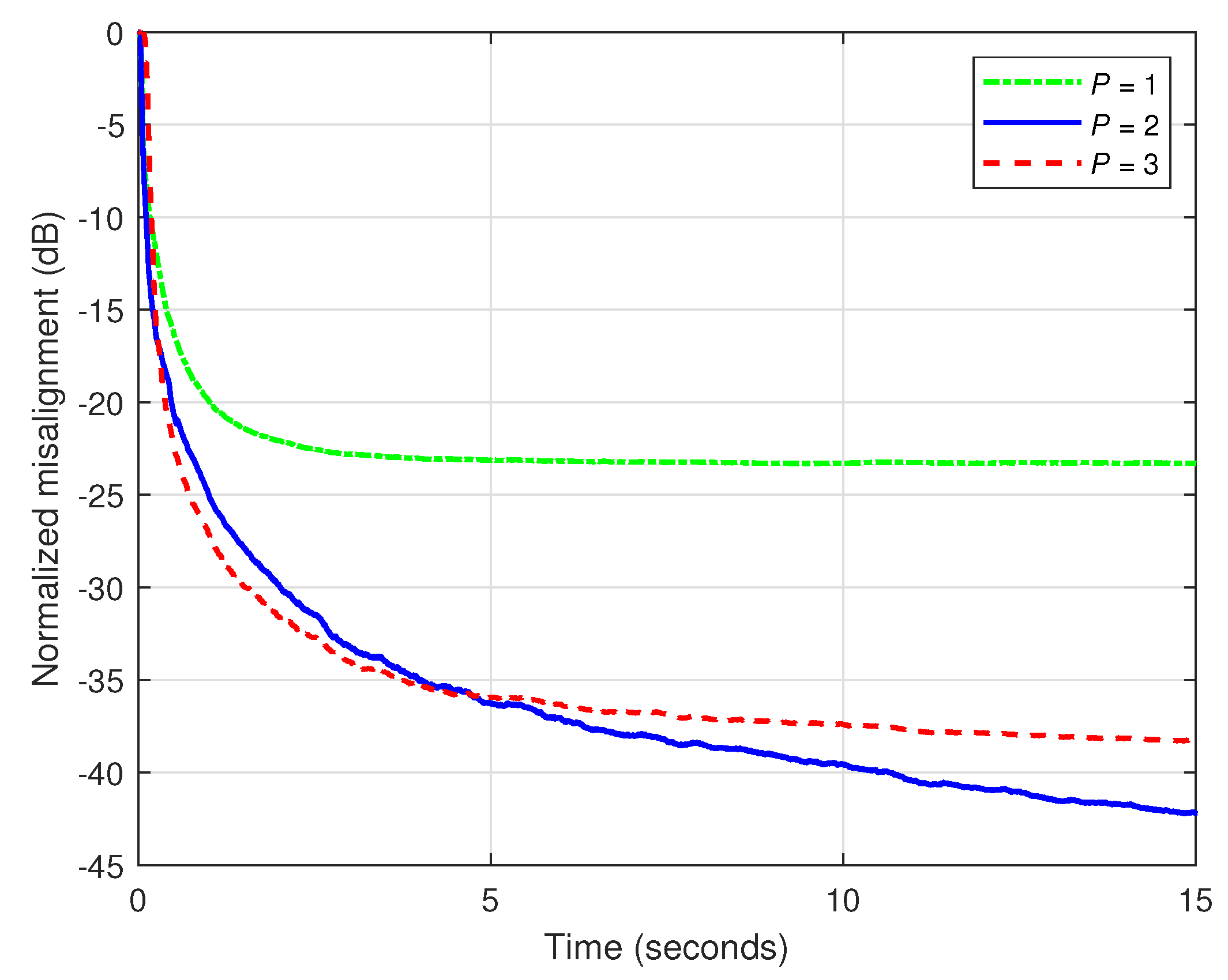
In the first set of experiments, we focus on the main parameters of KF-TOT in order to outline their influence on the overall performance of the algorithm. In these simulations, the input signal is an AR(1) process and dB. First, we assess the influence of the decomposition parameter P. As shown in [36], its values are usually much smaller than , while for network impulse responses (like the one involved in the experiments), the value of P is in the vicinity of . In Figure 1, three values of P are considered within the KF-TOT, while using null uncertainty parameters, i.e., . As explained in Section 3, this setting targets the best accuracy of the algorithm, i.e., the lowest misalignment, while sacrificing in terms of tracking (as shown in the next experiment). First, we can notice in Figure 1 that the KF-TOT using leads to a reasonable attenuation of the misalignment, with the smallest parameter space, i.e., using only 68 coefficients, according to the example provided in Section 2.3, related to (12). Increasing the value of P improves the performance of the KF-TOT, but up to a certain limit, which is related to the low-rank features of the impulse response to be identified. As we can notice in Figure 1, using and 3 leads to similar performances. Consequently, increasing the value of P beyond this limit will not bring additional gains. Moreover, two of the three component filters of KF-TOT have and coefficients, respectively. Hence, increasing the value of P also leads to a larger parameter space, which is not justified in terms of better performance. In our scenario, a value of represents a reasonable choice, taking into account the compromise between performance and complexity. In this case, the parameter space of KF-TOT comprises 132 coefficients (as also indicated in Section 2.3), still representing a significant reduction as compared to the length of the full impulse response.
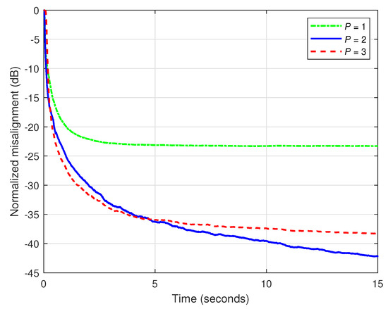
Figure 1.
Normalized misalignment of the KF-TOT using different values of P and null uncertainty parameters. The input signal is an AR(1) process and dB.
Next, in Figure 2, we analyze the tracking capabilities of the KF-TOT (with ) when using constant values of the uncertainties parameters. For the sake of simplicity, we generally denote these parameters by , where . The echo path changes after 15 s from the start of the experiment. As outlined in the previous simulation (related to Figure 1), the values lead to good accuracy, but poor tracking, as we can also notice in Figure 2. Reducing the values of improves the tracking but increases the misalignment (i.e., reduces the accuracy of the estimate). Consequently, a compromise should be considered between these main performance criteria.
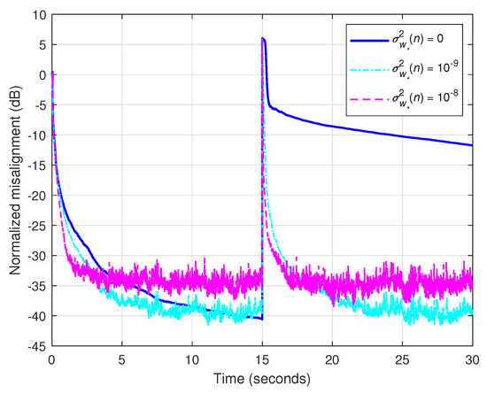
Figure 2.
Normalized misalignment of the KF-TOT using and different constant values of the uncertainty parameters. The input signal is an AR(1) process, dB, and the echo path changes after 15 s.
For this purpose, it would be useful to evaluate the uncertainties parameters within the algorithm, using a certain measure that captures the variation from to . A simple and practical way to assess this issue was proposed in [7], by computing in each iteration the quantity . Setting the values of in this manner allows a better compromise between convergence/tracking and misalignment, as outlined in the rest of the experiments from this section. In other words, a small difference between and indicates that the algorithm is in steady-state, where small values of should be used. On the other hand, a large difference between the estimates from two consecutive time indices requires a fast reaction of the algorithm, by increasing the values of .
4.2. Conventional Kalman Filter versus KF-TOT
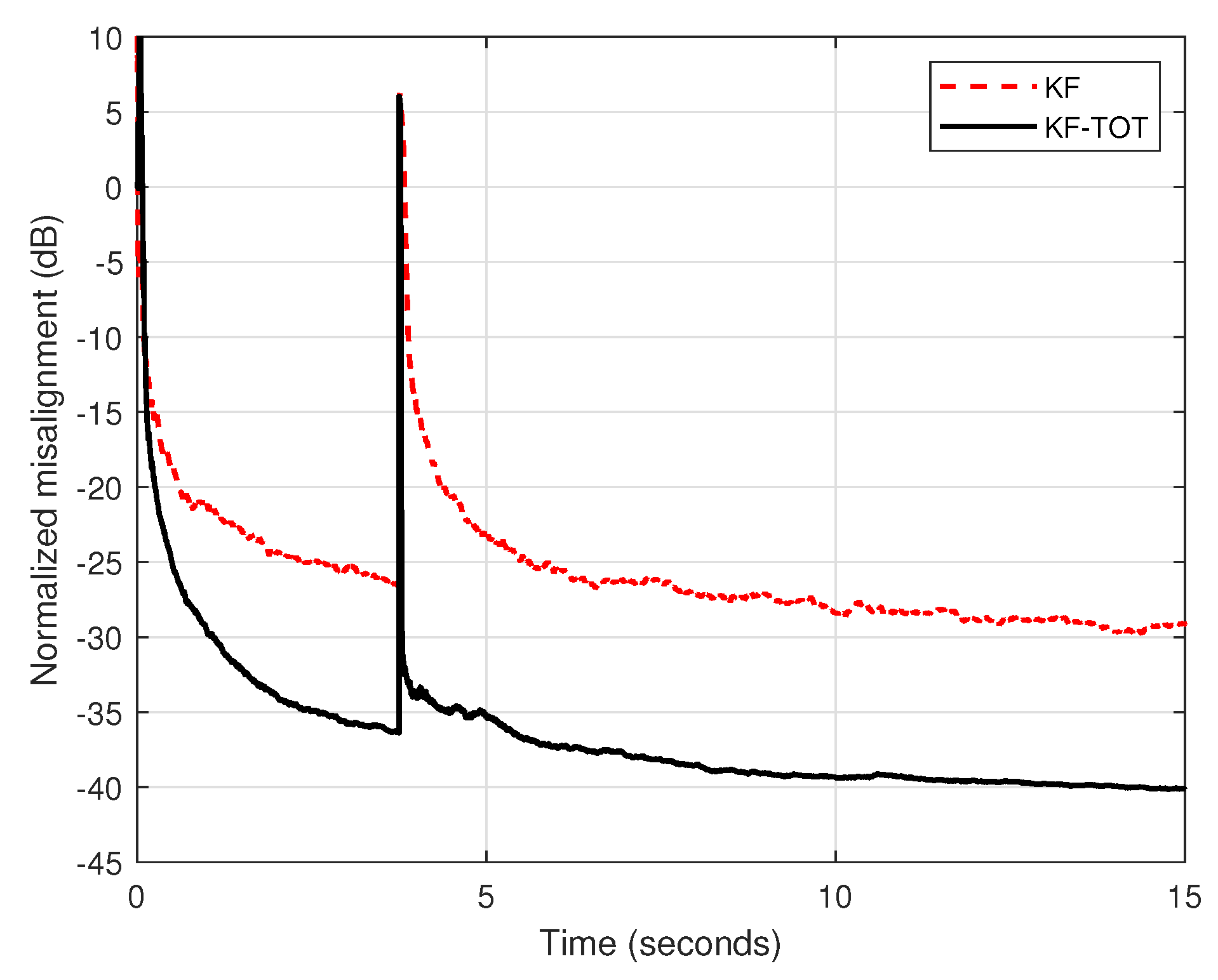
In the second set of experiments, we compare the performance of the conventional KF with the proposed KF-TOT (using ). For a fair comparison, both algorithms evaluate the uncertainty parameters in the same manner, as explained before. The input signal is an AR(1) process, the echo path changes after 3.75 s from the beginning of simulation, and different SNRs are used. First, in Figure 3, we set dB. As we can notice, the KF-TOT outperforms the conventional KF in terms of both performance criteria, i.e., convergence/tracking and misalignment. This is due to the fact that the conventional KF involves a single (long-length) filter, with , while the proposed KF-TOT combines the estimates provided by three (much) shorter filters, with , , and coefficients, respectively.
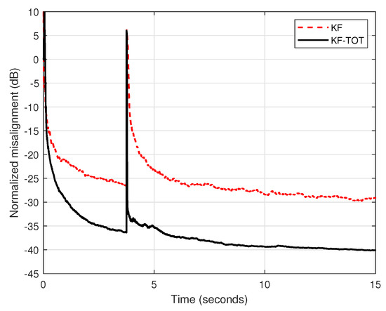
Figure 3.
Normalized misalignment of the conventional KF and KF-TOT (with ). The input signal is an AR(1) process, dB, and the echo path changes after 3.75 s.
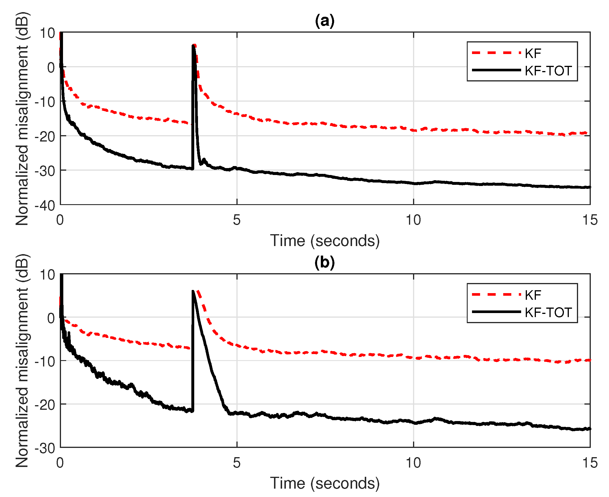
These performance gains are also valid in low SNR environments, as we can notice in Figure 4a,b, where the SNR is set to 10 dB and 0 dB, respectively. Even if there is a slightly slower tracking reaction of the KF-TOT in heavy noise conditions, like in Figure 4b, it still outperforms by far its conventional KF counterpart.

Figure 4.
Normalized misalignment of the conventional KF and KF-TOT (with ). The input signal is an AR(1) process, the echo path changes after 3.75 s: (a) dB and (b) dB.
4.3. KF-NKP versus KF-TOT
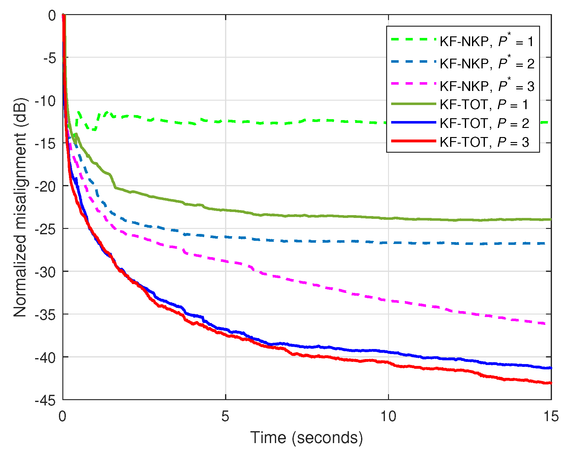
In the third set of experiments, the NKP-based version of the Kalman filter from [27] is involved in comparisons, namely, KF-NKP. This is also a decomposition-based algorithm, but exploits a second-order level, combining the solutions of two shorter filters of lengths and , where the length of the global filter is factorized as , while . In our scenario, since , we use the decomposition setup and . In Figure 5, the input signal is a speech sequence, dB, and different values of and P are used for the KF-NKP and KF-TOT, respectively. As we can notice, the KF-TOT outperforms the KF-NKP for all the corresponding values of the decomposition parameters. In the case of the KF-NKP, the value of is related to the rank of the corresponding matrix (of size ) associated with the reshaped impulse response [27]. In the case of the impulse response used in the experiments, this rank is equal to 3, so that increasing the value of beyond this value does not lead to any performance improvement.
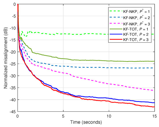
Figure 5.
Normalized misalignment of the KF-NKP [27] and KF-TOT, using different values of and P, respectively. The input signal is a speech sequence and dB.
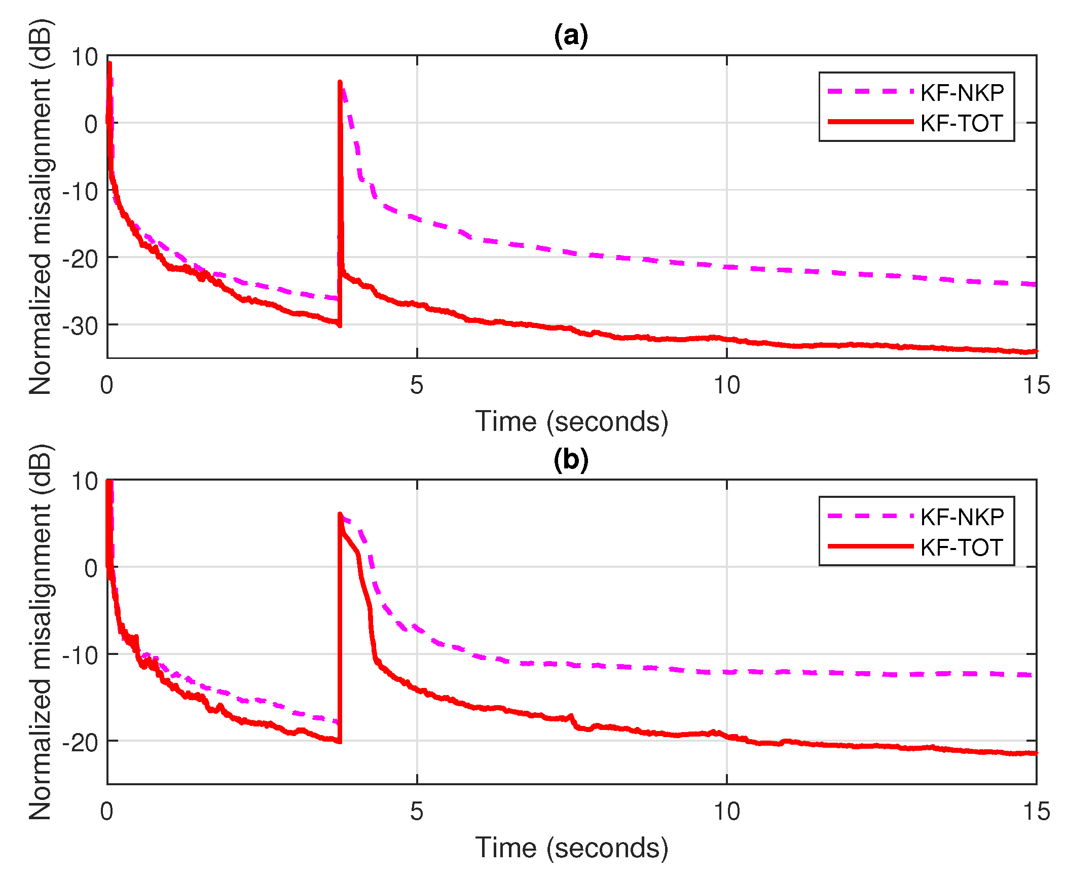
These decomposition-based Kalman filters are further analyzed in Figure 6, using lower SNRs and considering a change in the echo path (after 3.75 s). In both scenarios (i.e., dB and 0 dB), the proposed KF-TOT achieves better performance than the KF-NKP, in terms of both the tracking reaction and the misalignment level. Moreover, as supported in Figure 6b, the KF-TOT can operate with , while still outperforming its KF-NKP counterpart.
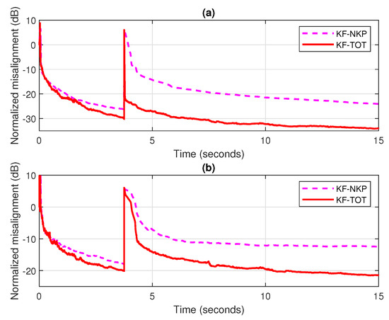
Figure 6.
Normalized misalignment of the KF-NKP [27] (with ) and KF-TOT (using different values of P). The input signal is a speech sequence, the echo path changes after 3.75 s: (a) dB, ; and (b) dB, .
4.4. RLS-TOT versus KF-TOT
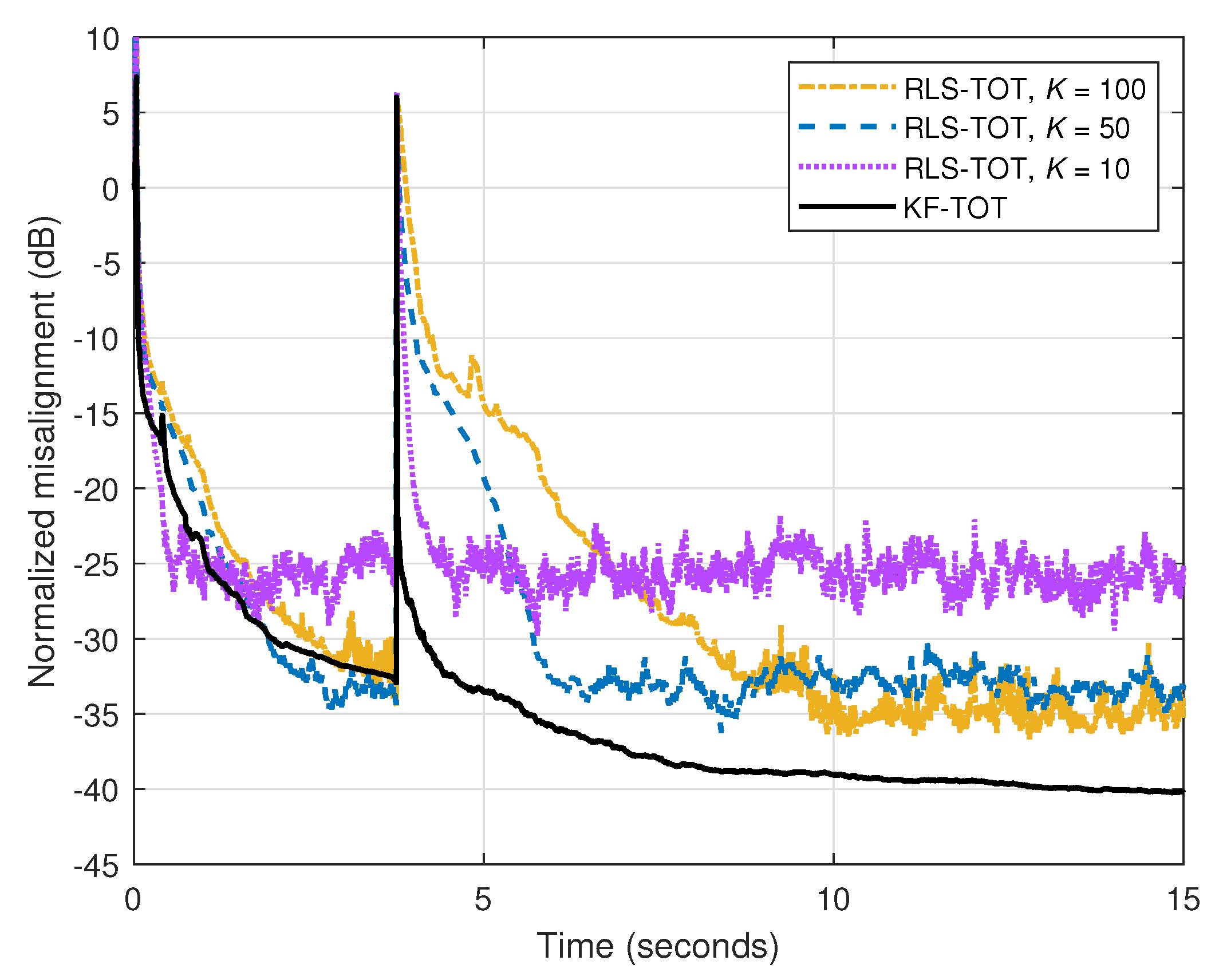
Finally, in the fourth set of experiments, the recently developed RLS-TOT [37] is involved in comparisons. It is known that there are inherent similarities between RLS-based algorithms and the Kalman filter [2,7]. However, due to its specific parameters, the Kalman filter allows a better control, especially in nonstationary conditions. In the case of the RLS-TOT, its overall performance is controlled in terms of the forgetting factors, denoted by , where . These are positive constants, which are smaller or equal to one. Larger values of (i.e., close or equal to one) lead to good accuracy of the filter estimate, thus reaching lower misalignment levels. On the other hand, the tracking reaction of the algorithm is reduced. This can be improved by decreasing the values of , while sacrificing in terms of accuracy (i.e., increasing the misalignment). In this context, a reliable compromise between these main performance criteria was proposed in [37], by using (which corresponds to the shortest filter of length ), while the other two forgetting factors are set according to and , with . In the scenario analyzed in Figure 7, different values of K are used for the RLS-TOT. The input signal is speech, dB, the echo path changes after 3.75 s, and both TOT-based algorithms use the same value of the decomposition parameter, which is set to . First, we can notice the compromise between the main performance criteria of the RLS-TOT (i.e., tracking versus misalignment) when using different values of K, i.e., different forgetting factors. On the other hand, the proposed KF-TOT achieves a much better tracking behavior, while still reaching a lower misalignment level.
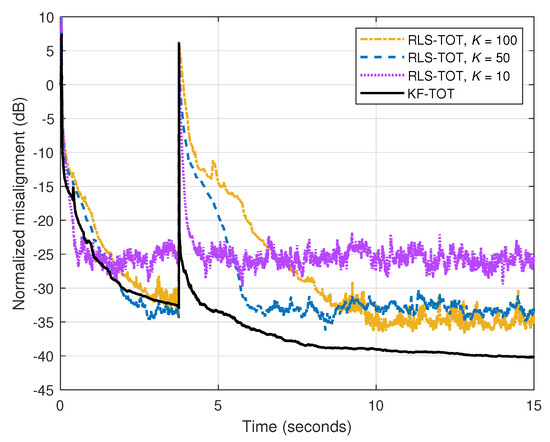
Figure 7.
Normalized misalignment of the RLS-TOT [37] (using different forgetting factors) and KF-TOT, with . The input signal is a speech sequence, dB, and the echo path changes after 3.75 s.
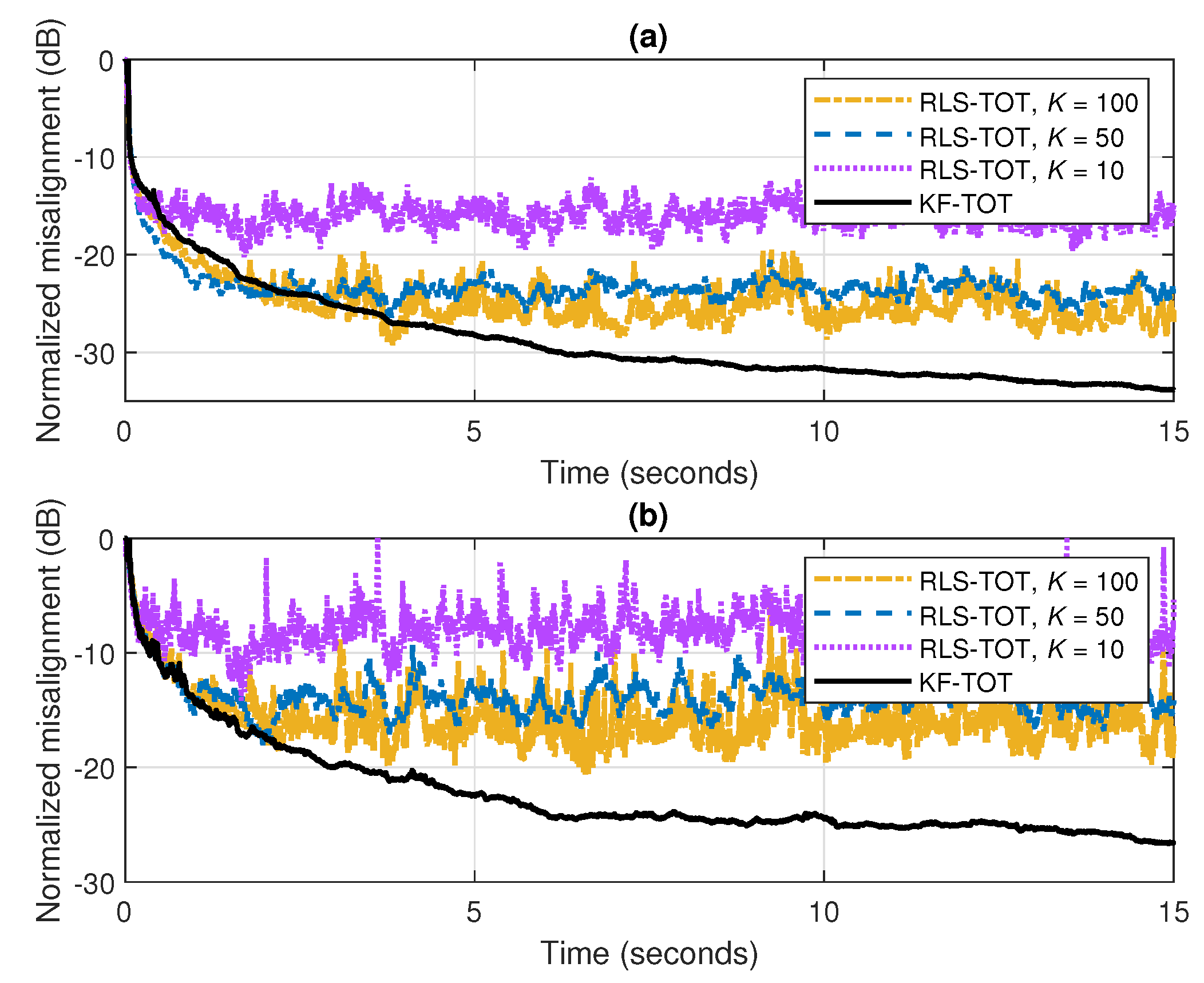
The accuracy of the solution provided by the KF-TOT can also be achieved in lower SNR environments, as supported in Figure 8a,b, where dB and 0 dB, respectively. The other conditions are basically the same as in the previous experiment, but without changing the echo path, in order to focus only on the accuracy of the estimate. As expected, increasing the values of the forgetting factors of RLS-TOT (i.e., increasing the values of K) leads to lower misalignment levels. Nevertheless, the KF-TOT provides a smooth convergence behavior toward a low steady-state misalignment level. To reach this accuracy, the forgetting factors of the RLS-TOT should be further increased, but the price to pay will be a poor tracking reaction in nonstationary environments (as previously outlined in Figure 7). Concluding, taking into account its overall performance, the KF-TOT represents a more reliable choice.
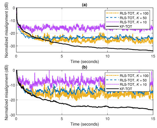
Figure 8.
Normalized misalignment of the RLS-TOT [37] (using different forgetting factors) and KF-TOT, with . The input signal is a speech sequence, while (a) dB and (b) dB.
5. Conclusions and Future Work
In the current paper, following the recently proposed TOT-based decomposition of the impulse response [36], we have developed a Kalman filter that exploits this technique, in the framework of system identification. The proposed KF-TOT combines (with the Kronecker product) the estimates provided by three filters, which can be much shorter as compared to the full length of the global impulse response. Since the length of an adaptive filter is related to its main performance criteria, this decomposition-based solution leads to important gains. As a result, following the announced goals from Section 1, the KF-TOT first outperforms the conventional Kalman filter in terms of both convergence rate and tracking, but also in terms of accuracy, reaching a significantly lower misalignment level. In addition, as supported in Table 1, these performance gains are achieved owning a lower computational complexity. Second, the KF-TOT leads to improved performances as compared to its KF-NKP counterpart [27], which exploits a second-order decomposition level by combining the estimates provided by two filters. Third, based on the evaluation of the KF-TOT as compared to the recently developed RLS-TOT [37], we reach the conclusion that the proposed algorithm is more reliable in nonstationary conditions, owning to a better tracking behavior and an improved accuracy of the solution.
Due to its performance features, the proposed KF-TOT fits very well for applications that involve the identification of long-length low-rank impulse responses, especially for time-varying systems. In this context, echo cancellation would represent an excellent application framework, since the echo paths (for both network and acoustic scenarios) are characterized by impulse responses that could easily reach hundreds/thousands of coefficients, while also being highly variable in time. Since this is a real-time application, a fast identification (and tracking) of the echo path impulse response, with low computational demands, would be a very appealing asset. In addition, different long-length low-rank systems can be involved in various applications, which include digital TV transmission [56], satellite-linked communications [57], underwater communications [58], and adaptive beamformers [59]. Hence, the developed KF-TOT could also represent a practical solution for such real-world applications.
Future work will focus on analyzing a higher-order decomposition level in conjunction with the Kalman filter. In this context, the main challenge is related to the way we handle the rank of a higher-order tensor that results from the development. Usually, approximation techniques are used to find such a tensor rank, which could represent a practical limitation. In the TOT framework, i.e., third-order decomposition level [36], the corresponding tensor associated with the reshaped impulse response results as a sum of P third-order tensors of rank , so this parameter is controlled and limited to small values. Since there is not a straightforward extension from one decomposition level to another, applying the decomposition technique to a higher order while still controlling the tensor rank represents a challenging task. Several preliminary ideas can be found in [60]. Also, we aim to involve the KF-TOT and the related decomposition-based algorithms in the framework of other applications that require the identification of long-length impulse responses, especially related to the acoustic domain.
Author Contributions
Conceptualization, L.-M.D.; methodology, C.P.; validation, J.B.; formal analysis, F.A. All authors have read and agreed to the published version of the manuscript.
Funding
The work of Constantin Paleologu and Felix Albu was supported by a grant of the Ministry of Research, Innovation and Digitization, CNCS–UEFISCDI, project number PN-III-P4-PCE-2021-0780, within PNCDI III.
Institutional Review Board Statement
Not applicable.
Informed Consent Statement
Not applicable.
Data Availability Statement
Data is contained within the article.
Conflicts of Interest
The authors declare no conflicts of interest.
References
- Kalman, R.E. A new approach to linear filtering and prediction problems. J. Basic Eng. 1960, 82, 35–45. [Google Scholar] [CrossRef]
- Sayed, A.H.; Kailath, T. A state-space approach to adaptive RLS filtering. IEEE Signal Process. Mag. 1994, 11, 18–60. [Google Scholar] [CrossRef]
- Faragher, R. Understanding the basis of the Kalman filter via a simple and intuitive derivation. IEEE Signal Process. Mag. 2012, 29, 128–132. [Google Scholar] [CrossRef]
- Enzner, G.; Vary, P. Frequency-domain adaptive Kalman filter for acoustic echo cancellation. Signal Process. 2006, 86, 1140–1156. [Google Scholar] [CrossRef]
- Enzner, G. Bayesian inference model for applications of time-varying acoustic system identification. In Proceedings of the 2010 18th EUSIPCO European Signal Processing Conference, Aalborg, Denmark, 23–27 August 2010; pp. 2126–2130. [Google Scholar]
- Malik, S.; Enzner, G. State-space frequency-domain adaptive filtering for nonlinear acoustic echo cancellation. IEEE Trans. Audio Speech Lang. Process. 2012, 20, 2065–2079. [Google Scholar] [CrossRef]
- Paleologu, C.; Benesty, J.; Ciochină, S. Study of the general Kalman filter for echo cancellation. IEEE Trans. Audio Speech Lang. Process. 2013, 21, 1539–1549. [Google Scholar] [CrossRef]
- Yang, F.; Enzner, G.; Yang, J. Frequency-domain adaptive Kalman filter with fast recovery of abrupt echo-path changes. IEEE Signal Process. Lett. 2017, 24, 1778–1782. [Google Scholar] [CrossRef]
- Enzner, G.; Voit, S. Hybrid-frequency-resolution adaptive Kalman filter for online identification of long acoustic responses with low input-output latency. IEEE/ACM Trans. Audio Speech Lang. Process. 2023, 31, 3550–3563. [Google Scholar] [CrossRef]
- Duttweiler, D.L. Proportionate normalized least-mean-squares adaptation in echo cancelers. IEEE Trans. Speech Audio Process. 2000, 8, 508–518. [Google Scholar] [CrossRef]
- Deng, H.; Doroslovački, M. Proportionate adaptive algorithms for network echo cancellation. IEEE Trans. Signal Process. 2006, 54, 1794–1803. [Google Scholar] [CrossRef]
- Loganathan, P.; Khong, A.W.; Naylor, P. A class of sparseness-controlled algorithms for echo cancellation. IEEE Trans. Audio Speech Lang. Process. 2009, 17, 1591–1601. [Google Scholar] [CrossRef]
- das Chagas de Souza, R.S.F.; Morgan, D.R. An enhanced IAF-PNLMS adaptive algorithm for sparse impulse response identification. IEEE Trans. Signal Process. 2012, 60, 3301–3307. [Google Scholar] [CrossRef]
- Liu, J.; Grant, S.L. Proportionate adaptive filtering for block-sparse system identification. IEEE/ACM Trans. Audio Speech Lang. Process. 2016, 24, 623–630. [Google Scholar] [CrossRef]
- Yang, Z.; Zheng, Y.R.; Grant, S.L. Proportionate affine projection sign algorithms for network echo cancellation. IEEE Trans. Audio Speech Lang. Process. 2011, 19, 2273–2284. [Google Scholar] [CrossRef]
- Zakharov, Y.V.; Nascimento, V.H. DCD-RLS adaptive filters with penalties for sparse identification. IEEE Trans. Signal Process. 2013, 61, 3198–3213. [Google Scholar] [CrossRef]
- Yu, Y.; Lu, L.; Zakharov, Y.; de Lamare, R.C.; Chen, B. Robust sparsity-aware RLS algorithms with jointly-optimized parameters against impulsive noise. IEEE Signal Process. Lett. 2022, 29, 1037–1041. [Google Scholar] [CrossRef]
- Comminiello, D.; Scarpiniti, M.; Azpicueta-Ruiz, L.A.; Arenas-García, J.; Uncini, A. Combined nonlinear filtering architectures involving sparse functional link adaptive filters. Signal Process. 2017, 135, 168–178. [Google Scholar] [CrossRef]
- Yu, Y.; Huang, Z.; He, H.; Zakharov, Y.; de Lamare, R.C. Sparsity-aware robust normalized subband adaptive filtering algorithms with alternating optimization of parameters. IEEE Trans. Circuits Syst. II Express Briefs 2022, 69, 3934–3938. [Google Scholar] [CrossRef]
- Yu, Y.; Ye, J.; Zakharov, Y.; He, H. Robust proportionate subband adaptive filter algorithms with optimal variable step-size. IEEE Trans. Circuits Syst. II Express Briefs 2024, 71, 2444–2448. [Google Scholar] [CrossRef]
- Zhang, Y.; Wu, T.; Zakharov, Y.V.; Li, J. MMP-DCD-CV based sparse channel estimation algorithm for underwater acoustic transform domain communication system. Appl. Acoust. 2019, 154, 43–52. [Google Scholar] [CrossRef]
- Niedźwiecki, M.; Gańcza, A.; Shen, L.; Zakharov, Y. Adaptive identification of sparse underwater acoustic channels with a mix of static and time-varying parameters. Signal Process. 2022, 200, 108664. [Google Scholar] [CrossRef]
- Liao, M.; Zakharov, Y.V. DCD-based joint sparse channel estimation for OFDM in virtual angular domain. IEEE Access 2021, 9, 102081–102090. [Google Scholar] [CrossRef]
- Radhika, S.; Albu, F.; Chandrasekar, A. Proportionate maximum Versoria criterion-based adaptive algorithm for sparse system identification. IEEE Trans. Circuits Syst. II Express Briefs 2022, 69, 1902–1906. [Google Scholar] [CrossRef]
- Paleologu, C.; Benesty, J.; Ciochină, S. Linear system identification based on a Kronecker product decomposition. IEEE/ACM Trans. Audio Speech Lang. Process. 2018, 26, 1793–1808. [Google Scholar] [CrossRef]
- Elisei-Iliescu, C.; Paleologu, C.; Benesty, J.; Stanciu, C.; Anghel, C.; Ciochină, S. Recursive least-squares algorithms for the identification of low-rank systems. IEEE/ACM Trans. Audio Speech Lang. Process. 2019, 27, 903–918. [Google Scholar] [CrossRef]
- Dogariu, L.-M.; Paleologu, C.; Benesty, J.; Ciochină, S. An efficient Kalman filter for the identification of low-rank systems. Signal Process. 2020, 166, 107239. [Google Scholar] [CrossRef]
- Bhattacharjee, S.S.; George, N.V. Nearest Kronecker product decomposition based normalized least mean square algorithm. In Proceedings of the 2020 IEEE International Conference on Acoustics, Speech and Signal Processing (ICASSP), Barcelona, Spain, 4–8 May 2020; pp. 476–480. [Google Scholar]
- Bhattacharjee, S.S.; Kumar, K.; George, N.V. Nearest Kronecker product decomposition based generalized maximum correntropy and generalized hyperbolic secant robust adaptive filters. IEEE Signal Process. Lett. 2020, 27, 1525–1529. [Google Scholar] [CrossRef]
- Bhattacharjee, S.S.; George, N.V. Nearest Kronecker product decomposition based linear-in-the-parameters nonlinear filters. IEEE/ACM Trans. Audio Speech Lang. Process. 2021, 29, 2111–2122. [Google Scholar] [CrossRef]
- Bhattacharjee, S.S.; Patel, V.; George, N.V. Nonlinear spline adaptive filters based on a low rank approximation. Signal Process. 2022, 201, 108726. [Google Scholar] [CrossRef]
- Nezamdoust, A.; Huemer, M.; Uncini, A.; Comminiello, D. Efficient functional link adaptive filters based on nearest Kronecker product decomposition. In Proceedings of the IEEE ICASSP, Seoul, Republic of Korea, 14–19 April 2024; pp. 886–890. [Google Scholar]
- Bhattacharjee, S.S.; George, N.V. Fast and efficient acoustic feedback cancellation based on low rank approximation. Signal Process. 2021, 182, 107984. [Google Scholar] [CrossRef]
- Vadhvana, S.; Yadav, S.K.; Bhattacharjee, S.S.; George, N.V. An improved constrained LMS algorithm for fast adaptive beamforming based on a low rank approximation. IEEE Trans. Circuits Syst. II Express Briefs 2022, 69, 3605–3609. [Google Scholar] [CrossRef]
- Dogariu, L.-M.; Benesty, J.; Paleologu, C.; Ciochină, S. Identification of room acoustic impulse responses via Kronecker product decompositions. IEEE/ACM Trans. Audio Speech Lang. Process. 2022, 30, 2828–2841. [Google Scholar] [CrossRef]
- Benesty, J.; Paleologu, C.; Ciochină, S. Linear system identification based on a third-order tensor decomposition. IEEE Signal Process. Lett. 2023, 30, 503–507. [Google Scholar] [CrossRef]
- Paleologu, C.; Benesty, J.; Stanciu, C.L.; Jensen, J.R.; Christensen, M.G.; Ciochină, S. Recursive least-squares algorithm based on a third-order tensor decomposition for low-rank system identification. Signal Process. 2023, 213, 109216. [Google Scholar] [CrossRef]
- Kolda, T.G.; Bader, B.W. Tensor decompositions and applications. SIAM Rev. 2009, 51, 455–500. [Google Scholar] [CrossRef]
- Comon, P. Tensors: A brief introduction. IEEE Signal Process. Mag. 2014, 31, 44–53. [Google Scholar] [CrossRef]
- Cichocki, A.; Mandic, D.P.; Phan, A.; Caiafa, C.F.; Zhou, G.; Zhao, Q.; Lathauwer, L.D. Tensor decompositions for signal processing applications: From two-way to multiway component analysis. IEEE Signal Process. Mag. 2015, 32, 145–163. [Google Scholar] [CrossRef]
- Vervliet, N.; Debals, O.; Sorber, L.; Lathauwer, L.D. Breaking the curse of dimensionality using decompositions of incomplete tensors: Tensor-based scientific computing in big data analysis. IEEE Signal Process. Mag. 2014, 31, 71–79. [Google Scholar] [CrossRef]
- Becker, H.; Albera, L.; Comon, P.; Gribonval, R.; Wendling, F.; Merlet, I. Brain-source imaging: From sparse to tensor models. IEEE Signal Process. Mag. 2015, 32, 100–112. [Google Scholar] [CrossRef]
- Bousse, M.; Debals, O.; Lathauwer, L.D. A tensor-based method for large-scale blind source separation using segmentation. IEEE Trans. Signal Process. 2017, 65, 346–358. [Google Scholar] [CrossRef]
- Sidiropoulos, N.; Lathauwer, L.D.; Fu, X.; Huang, K.; Papalexakis, E.; Faloutsos, C. Tensor decomposition for signal processing and machine learning. IEEE Trans. Signal Process. 2017, 65, 3551–3582. [Google Scholar] [CrossRef]
- Haykin, S. Adaptive Filter Theory, 4th ed.; Prentice-Hall: Upper Saddle River, NJ, USA, 2002. [Google Scholar]
- Sayed, A.H. Adaptive Filters; Wiley: New York, NY, USA, 2008. [Google Scholar]
- Diniz, P.S.R. Adaptive Filtering: Algorithms and Practical Implementation, 4th ed.; Springer: New York, NY, USA, 2013. [Google Scholar]
- Hänsler, E.; Schmidt, G. Acoustic Echo and Noise Control—A Practical Approach; Wiley: Hoboken, NJ, USA, 2004. [Google Scholar]
- Kay, S.M. Fundamentals of Statistical Signal Processing, Volume I: Estimation Theory; Prentice Hall: Englewood Cliffs, NJ, USA, 1993. [Google Scholar]
- Loan, C.F.V. The ubiquitous Kronecker product. J. Comput. Appl. Math. 2000, 123, 85–100. [Google Scholar] [CrossRef]
- Bertsekas, D.P. Nonlinear Programming, 2nd ed.; Athena Scientific: Belmont, MA, USA, 1999. [Google Scholar]
- Rupp, M.; Schwarz, S. Gradient-based approaches to learn tensor products. In Proceedings of the in 2015 23rd European Signal Processing Conference (EUSIPCO), Nice, France, 31 August–4 September 2015; pp. 2486–2490. [Google Scholar]
- Rupp, M.; Schwarz, S. A tensor LMS algorithm. In Proceedings of the 2015 IEEE International Conference on Acoustics, Speech and Signal Processing (ICASSP), South Brisbane, Australia, 19–24 April 2015; pp. 3347–3351. [Google Scholar]
- Iqbal, M.A.; Grant, S.L. Novel variable step size NLMS algorithm for echo cancellation. In Proceedings of the 2008 IEEE International Conference on Acoustics, Speech and Signal Processing (ICASSP), Las Vegas, NV, USA, 31 March–4 April 2008; pp. 241–244. [Google Scholar]
- Digital Network Echo Cancellers, ITU-T Recommendation G.168. 2012. Available online: www.itu.int/rec/T-REC-G.168 (accessed on 19 May 2024).
- Schreiber, W.F. Advanced television systems for terrestrial broadcasting: Some problems and some proposed solutions. Proc. IEEE 1995, 83, 958–981. [Google Scholar] [CrossRef]
- Steingass, A.; Lehner, A.; Perez-Fontan, F.; Kubista, E.; Arbesser-Rastburg, B. Characterization of the aeronautical satellite navigation channel through high-resolution measurement and physical optics simulation. Int. J. Satell. Commun. Netw. 2008, 26, 1–30. [Google Scholar] [CrossRef]
- Zhang, Y.; Zakharov, Y.V.; Li, J. Soft-decision-driven sparse channel estimation and turbo equalization for MIMO underwater acoustic communications. IEEE Access 2018, 6, 4955–4973. [Google Scholar]
- Ribeiro, L.N.; de Almeida, A.L.F.; Mota, J.C.M. Separable linearly constrained minimum variance beamformers. Signal Process. 2019, 158, 15–25. [Google Scholar] [CrossRef]
- Benesty, J.; Paleologu, C.; Dogariu, L.M. An iterative Wiener filter based on a fourth-order tensor decomposition. Symmetry 2013, 15, 1560. [Google Scholar] [CrossRef]

Disclaimer/Publisher’s Note: The statements, opinions and data contained in all publications are solely those of the individual author(s) and contributor(s) and not of MDPI and/or the editor(s). MDPI and/or the editor(s) disclaim responsibility for any injury to people or property resulting from any ideas, methods, instructions or products referred to in the content. |
© 2024 by the authors. Licensee MDPI, Basel, Switzerland. This article is an open access article distributed under the terms and conditions of the Creative Commons Attribution (CC BY) license (https://creativecommons.org/licenses/by/4.0/).