Abstract
Targeting the challenge of variable working conditions in bearing fault diagnosis, most of the fault diagnosis methods based on transfer learning focus on the transfer of knowledge, resulting in a poor diagnosis effect in the target domain. To solve the problem of transfer performance degradation, a multi-perception graph convolution transfer network (MPGCTN) is proposed. The MPGCTN is composed of a graph generation module, graph perception module, and domain discrimination module. In the graph generation module, a one-dimensional convolution neural network (1-D CNN) is used to extract features from the input, and then the structural features of samples are mined in the graph generation layer to construct the sample graph. In the following graph perception module, a multi-perception graph convolution network is designed to model the sample graph and learn the data structure information of the sample. Finally, in the domain discrimination module, the method is used to align the structural differences of the case graphs in different domains. Experimental results from experiments on Case Western Reserve University (CWRU) and Paderborn University (PU) bearing datasets show that the proposed method is effective and superior.
1. Introduction
Rotating machinery is widely used in manufacturing, energy supply, rail transit, aerospace, and other industries and plays a fundamental role in industrial production [1]. As an important part of rotating machinery, bearings are a kind of mechanical part that is used to reduce friction between other moving parts. Rotating machinery performance can be significantly impacted by bearing failures, particularly under severe working conditions [2]. The incorrect handling of these failures can pose a serious threat to personal safety and have a major impact on social and economic development [3]. Therefore, to maintain a safe operating environment and ensure high production efficiency, it is crucial to accurately identify the health status of the bearings.
The emergence of the industrial big data age has led to the collection and utilization of vast numbers of operational data in industrial production, which has accelerated the development of artificial intelligence techniques for fault diagnostics [4]. It has been difficult to meet the requirements of rapid and accurate diagnosis with traditional signal-based and model-based fault diagnosis methods, such as wavelet transform, state estimation methods, and so on [5,6]. In order to automatically extract fault features and implement high-efficiency diagnosis, deep learning (DL)-based diagnosis methods have become research hotspots in recent years [7,8]. Compared with traditional methods based on signal analysis and machine learning, DL-based diagnosis methods can reduce human experience interference and have more advantages in the field of intelligent diagnosis [9,10]. In addition, deep learning has further evolved to encompass transfer learning, federated learning, meta-learning, and other advanced paradigms [11]. These developments have significantly contributed to the enhancement of fault diagnosis methodologies, enabling the extraction of intricate fault features and the realization of high-efficiency diagnostic capabilities.
Currently, the following presumptions underlie effective applications of DL-based methods: (1) The fault samples are drawn from the same distribution of data; (2) A significant quantity of excellently labeled samples with faults is needed. Nevertheless, it is challenging to meet these presumptions in actual industrial scenarios due to the following issues: (1) Samples acquired under various conditions will have different distributions due to variations in working conditions, equipment wear, and ambient noise. In the end, diagnostic performance deteriorates when a model trained under one situation is applied to another; (2) Only a small number of fault data are available under particular operating conditions, and it is challenging to gather substantial historical fault data in advance [12]. The use of intelligent defect diagnostic techniques in industry is restricted by these issues.
Transfer learning (TL) aims to address the shortcomings of deep learning in fault diagnosis and offers a feasible and promising resolution [13]. TL allows models to apply knowledge learned from one task to another related task. As one of the important branches of TL, domain adaptation (DA) [14] transfers knowledge by narrowing the gap between two domains and learning domain-invariant features. In the application of bearing fault diagnosis, Huang et al. [15] developed a multi-source dense adaptation countermeasure network suitable for bearing fault diagnosis through integrated fusion. Jiao et al. [16] constructed a shared feature generator network and double classifier network, added additional classifier differences to the adversarial domain adaption network, and achieved more effective cross-domain diagnosis in a domain distribution transfer scenario. Kuang et al. [17] built an adversarial transfer learning network to diagnose data pertaining to class imbalance. Through adversarial training, they acquired information about class separation diagnosis for unbalanced data, and, through joint-distributed two-layer adversarial transfer learning, they acquired domain-invariant knowledge. While transfer-learning-based fault diagnosis techniques have shown promise, existing strategies primarily focus on minimizing distributional differences, overlooking variations in the underlying data structure of fault features. This oversight limits their effectiveness in capturing crucial structural information, thereby hindering performance in cross-domain fault diagnosis tasks.
To address these limitations, a multi-perception graph convolution transfer network (MPGCTN) is proposed. Unlike previous methods, the MPGCTN not only aims to minimize distributional differences but also aims to capture the intricate data structures inherent in fault features, which is effective for variable-working-condition bearing fault diagnosis across different domains. Central to the MPGCTN is the multi-perception graph convolutional network (MPGCN), which leverages multiple receptive fields to extract robust feature representations from complex data relationships. By integrating class labels, domain labels, and data structures into its architecture, the MPGCTN facilitates high-performance domain adaptation by effectively modeling the inherent characteristics of fault data. Specifically, the MPGCTN comprises three key modules: a graph generation module, a graph perception module, and a domain discrimination module. In the graph generation module, a one-dimensional CNN (1-D CNN) is used to capture features from the input, and then the instance graph is constructed through the graph generation layer. Then, in the graph perception module, the proposed MPGCN is utilized to identify the fault features that are hidden in the relationship data between nodes with varying scales. Finally, in the domain discrimination module, adversarial training of the classifier and domain discriminator is conducted to reduce structural differences between target domain and source domain samples for cross-domain diagnosis. Twelve transmission fault diagnosis tasks are constructed using two types of bearing datasets with four different working conditions to verify the effectiveness of this method. The following are the primary contributions of the suggested method:
(1) A multi-perception graph convolution transfer network (MPGCTN) is proposed which models class labels, domain labels, and data structure in deep networks and which achieves high-performance domain adaptation;
(2) A multi-perception graph convolutional network (MPGCN) is proposed to obtain a more robust feature representation by aggregating features learned from multiple receptive fields;
(3) The proposed method is evaluated on a cross-domain task of variable working conditions on two test platforms. Comparing the MPGCTN to other approaches, the results demonstrate its superior performance.
The rest of this paper is structured as follows: Section 2 presents a concise overview of key concepts and theoretical foundations concerning graph convolution networks and domain adaptation. The method proposed in this study is thoroughly introduced in Section 3. In Section 4, a comparative analysis of the proposed model and a variety of other models is conducted using the CWRU and PU datasets. The paper’s conclusion and future directions are covered in Section 5.
2. Preliminaries
A summary of the pertinent research is given in this section. Domain adaptation techniques are presented after some fundamental concepts of graph convolution networks are covered. These form the basis of our study.
2.1. Graph Convolution Network
Convolution neural networks (CNNs) have been extensively employed in various areas, including image recognition and natural language processing [18]. However, they are limited to processing normal Euclidean data, such as grids and sequences, and are unable to process non-Euclidean data, like knowledge graph data, efficiently. Traditional CNNs have trouble processing such network structure data since the graph’s structure is typically quite unpredictable, each node’s surrounding structure can be distinct, and its associated edges and neighboring nodes differ. The graph convolution neural network (GCN) is a CNN application for non-Euclidean graph-structured data [19].
GCN methods can be divided into two main categories: spectrum based and space based. From the standpoint of graph signal processing, the spectrum-based methods describe graph convolution by introducing a filter. The neighborhood-based feature information is aggregated in the space-based methods’ representations of graph convolution.
In graph theory, the relationship between nodes can be expressed as a relation graph , where G represents a graph, V is the set of vertices in the graph G, and E is the set of edges in the graph G.
In a spectrum-based GCN, graphs are assumed to be undirected, and one robust mathematical representation of undirected graphs is the regularized graph Laplacian matrix, as shown below.
where is the identity matrix, A is the adjacency matrix of the graph, D is the diagonal matrix, and . The eigenvalue decomposition of this Laplacian matrix L is
where is a diagonal matrix composed of eigenvalues of L, and the orthogonal matrix U is composed of eigenvectors of L.
The basic principle of the GCN is as follows. Taking into account the convolution operation , where g is the convolution kernel and x are the eigenvectors of the node, with the Fourier transform, the frequency domain form of the above convolution operation can be expressed as follows:
where represents the Fourier transform of x, and ⊙ is the Hadamard product.
can also be expressed as a diagonal matrix . Formula (3) can be simplified as follows:
where represents the map filter of N parameters to be trained.
However, directly training a set of N parameters is a lot of calculations. To simplify the calculation, Defferrard et al. [20] used Chebyshev polynomials to approximate graph convolution filters. In the network, the vertex embedding can be calculated according to the K-th Chebyshev polynomial, which is represented as follows:
where K is the largest order of the Chebyshev polynomial, is the rescaled eigenvalue, represents the largest eigenvalue, is the vector of the coefficients of the polynomial, and is the vector of the Chebyshev coefficients. is a Chebyshev polynomial of order k.
Following the Chebyshev polynomial approximation of the filter, the graph convolution of node characteristics with the filter may be expressed mathematically as follows:
where is the rescaled Laplacian matrix.
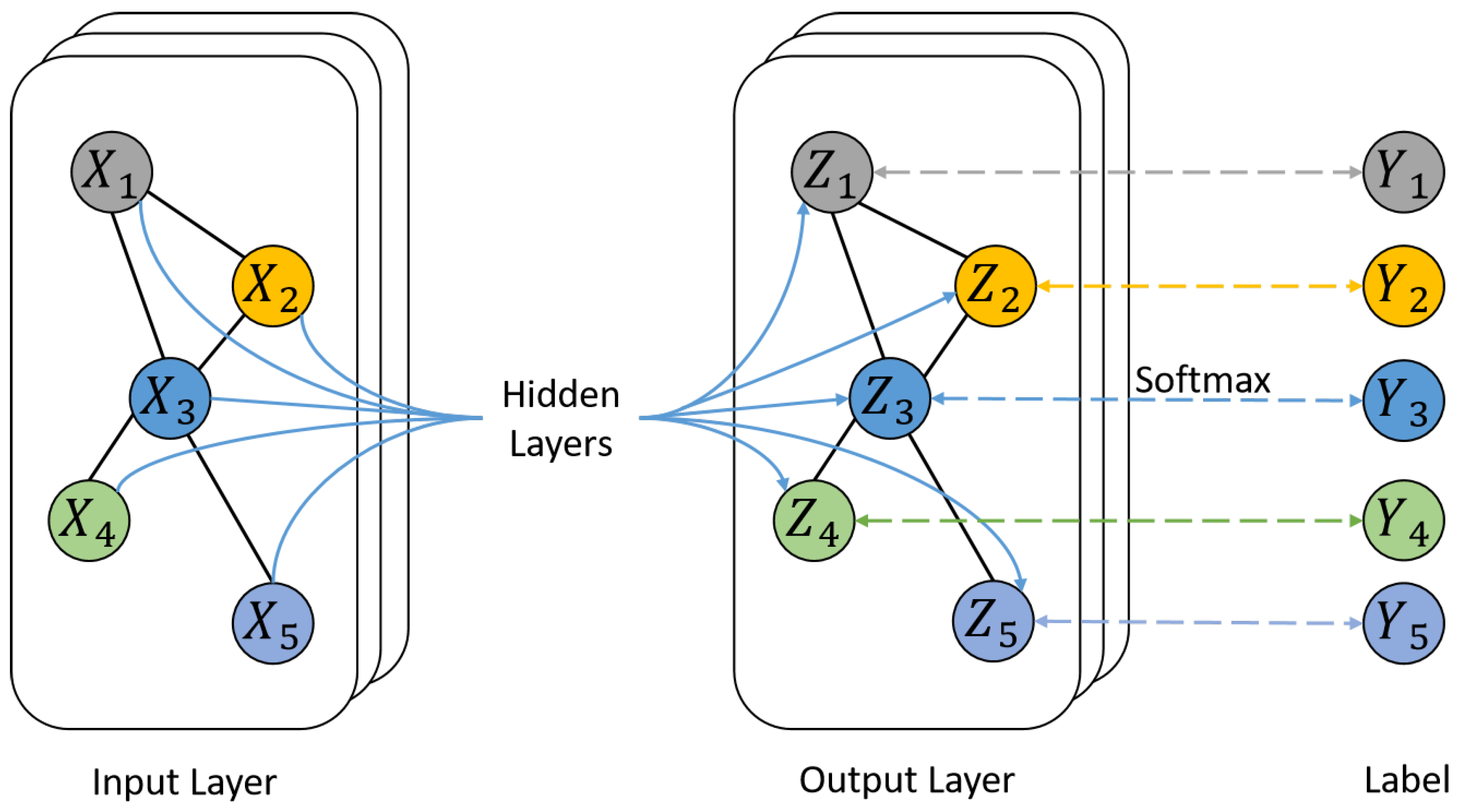
The standard two-layer graph convolution network model for node classification is shown in Figure 1, which can be expressed as follows:
where is a collection of node features, and n is the number of nodes. It can be seen from Figure 1 that the essence of the graph convolution neural network is to aggregate the characteristics of neighbor nodes and perform graph learning through the relationship between nodes, and tasks such as node classification and graph classification can be realized.
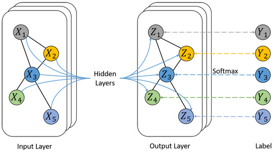
Figure 1.
A typical graph convolution network structure consisting of two graph convolution layers.
2.2. Domain Adaptation
In the practical application of transfer learning, the model trained by the source domain can help the target domain train in the absence of sample labels [21]. Domain shift resulting from discrepancies in data distribution across source and target domains becomes difficult in this scenario. However, domain adaptation techniques assist in alleviating this problem.
Unsupervised domain adaptation is an important research field in domain adaptation [22]. In order to illustrate this problem clearly, the basic standard notation of domain adaptation is introduced. A domain is set, where is a feature space, and is the marginal distribution of data in the feature space. Given a labeled source domain and an unlabeled target domain , the feature space and label space Y of the two domains are the same, , , while the probability distribution is different, . In this case, the potential representation of the source domain data can be learned through feature extraction and representation learning of the source domain data. These potential representations are then applied to the target domain data.
For unsupervised domain adaptation, one of the most popular techniques is the domain adversarial neural network (DANN) [23]. The core idea of the domain adversarial adaptation method is to learn a good enough representation to reduce the difference in edge distribution between the source domain and the target domain at the representation level. Inspired by Generative Adversarial Networks (GANs) [24], a DANN uses domain discriminators to distinguish features generated by different data domains, and the adversarial loss of domain discriminators is as follows:
where is a feature extractor, and z represents the extracted features. The accuracy of the domain discriminator depicts the difference of the edge distribution of the two data domains. The DANN tries to deceive the domain discriminator by using the feature extractor, thereby reducing the difference in the edge distribution. The overall loss is expressed as follows:
With this adversarial learning strategy, domain-invariant features can be learned when domain discriminators cannot distinguish correctly. In order to realize knowledge transfer effectively, a DANN is adopted as the domain adaptation method.
3. Proposed Method
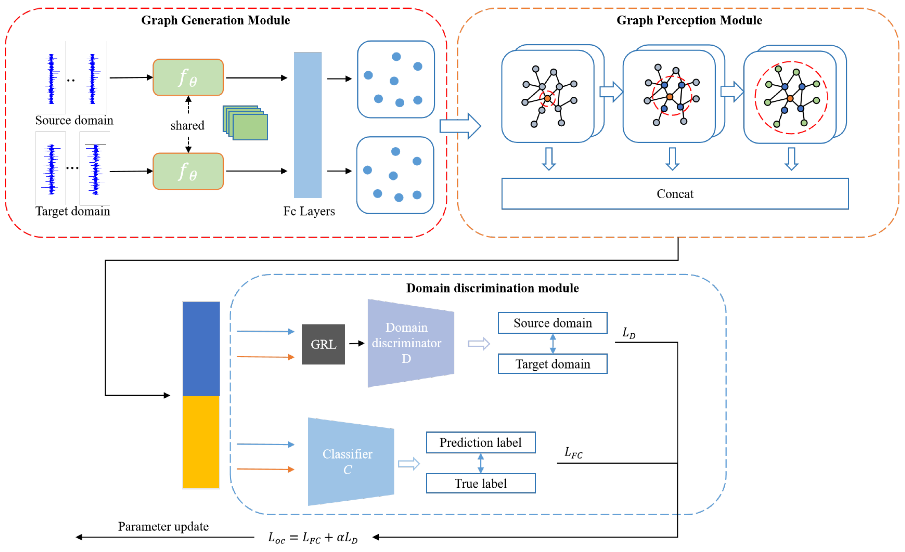
The proposed MPGCTN is introduced mainly in this section, including a graph generation module, a graph perception module, and a domain discrimination module, as shown in Figure 2. The raw data are input into the graph generation module, and the features are extracted by the CNN first. The graph generation layer is then used to automatically generate the association graphs. After that, the obtained graphs are input into the graph perception module, and the proposed multi-perception graph neural network can embed multi-dimensional data structure information into node features. Ultimately, domain discrimination and fault classification are performed using the acquired node attributes. A detailed flowchart of the proposed MPGCTN for achieving cross-domain fault diagnosis is shown in Figure 3.
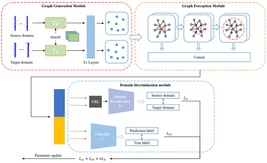
Figure 2.
MPGCTN structure diagram.

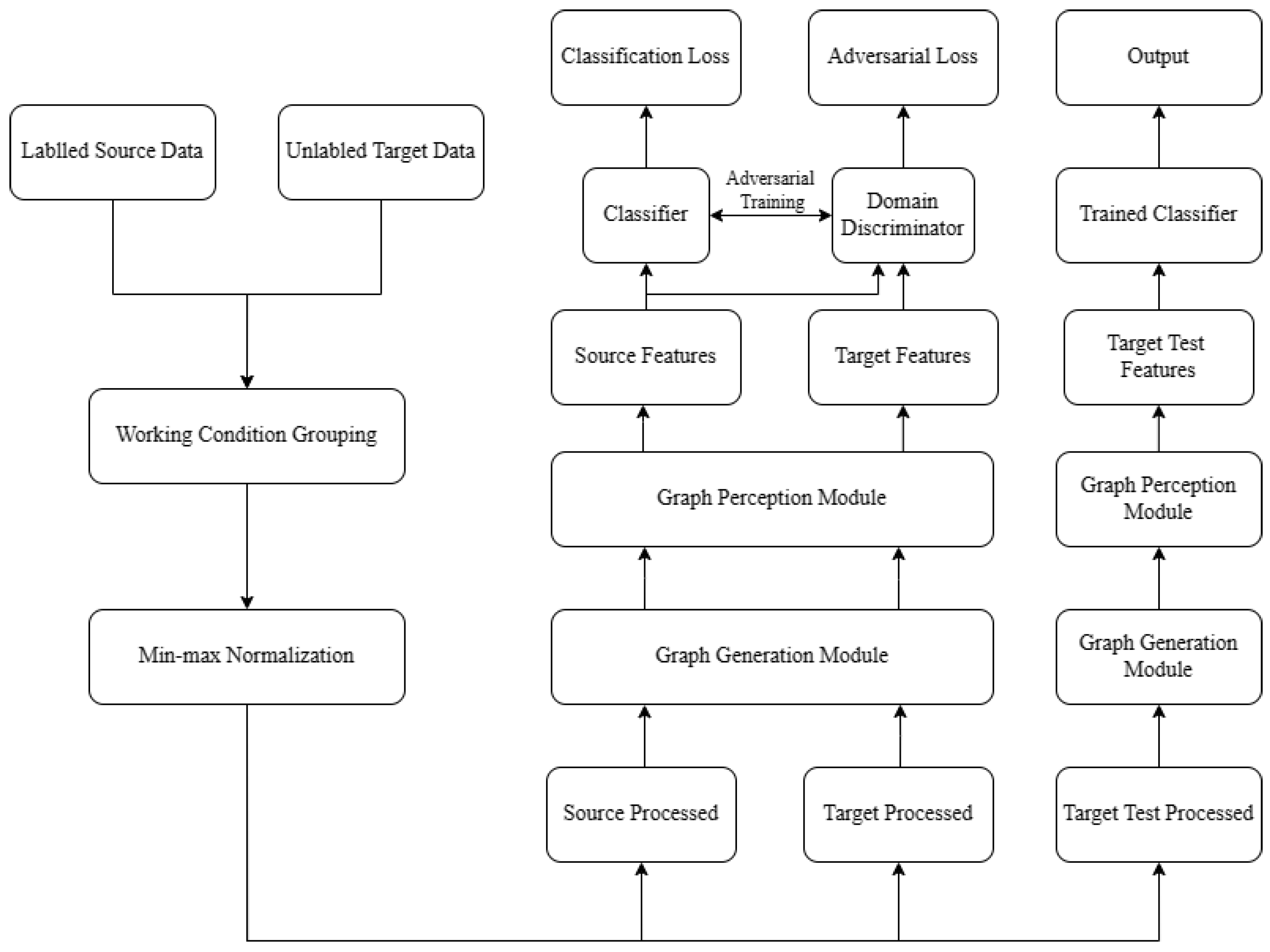
Figure 3.
Flowchart of the proposed method.
3.1. Graph Generation Module
The raw data need to be processed to build a graph data sample before the data can be used for graph neural network learning. Graph generation consists of two key components: adjacency matrix A and node feature matrix X. In order to obtain the node feature matrix X, the features are first captured from the input data using a 1-D CNN. The mapping for extracting features can be represented as follows:
where f represents the extracted features, F represents the 1-D CNN, and represents the input data.
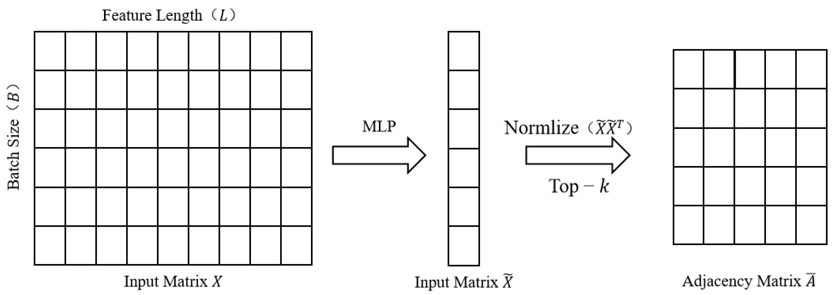
Zhao et al. [24] proposed a graph generation layer (GGL) to obtain the adjacency matrix A. Features can obtain the adjacency matrix A through the GGL and use the input matrix to construct an example graph. The process is shown in Figure 4.
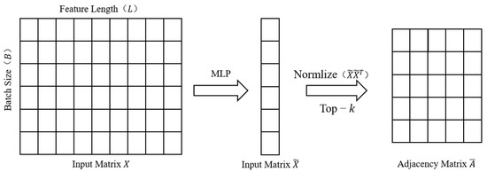
Figure 4.
Process of the graph generation.
The feature matrix is first input into the multilayer perceptron (MLP). Subsequently, the adjacency matrix is obtained through matrix multiplication between the MLP features and their transpositions. Finally, utilizing a top-k sorting mechanism, the first k-closest neighbors of each node are selected. Thus, the adjacency matrix can be derived using the following formula:
where A is the constructed adjacency matrix, and is the output of the MLP. is a sparse adjacency matrix that returns the indices of the maximum values of k of A in rows, which decreases the computational load and produces a sparse adjacency matrix.
3.2. Graph Perception Module
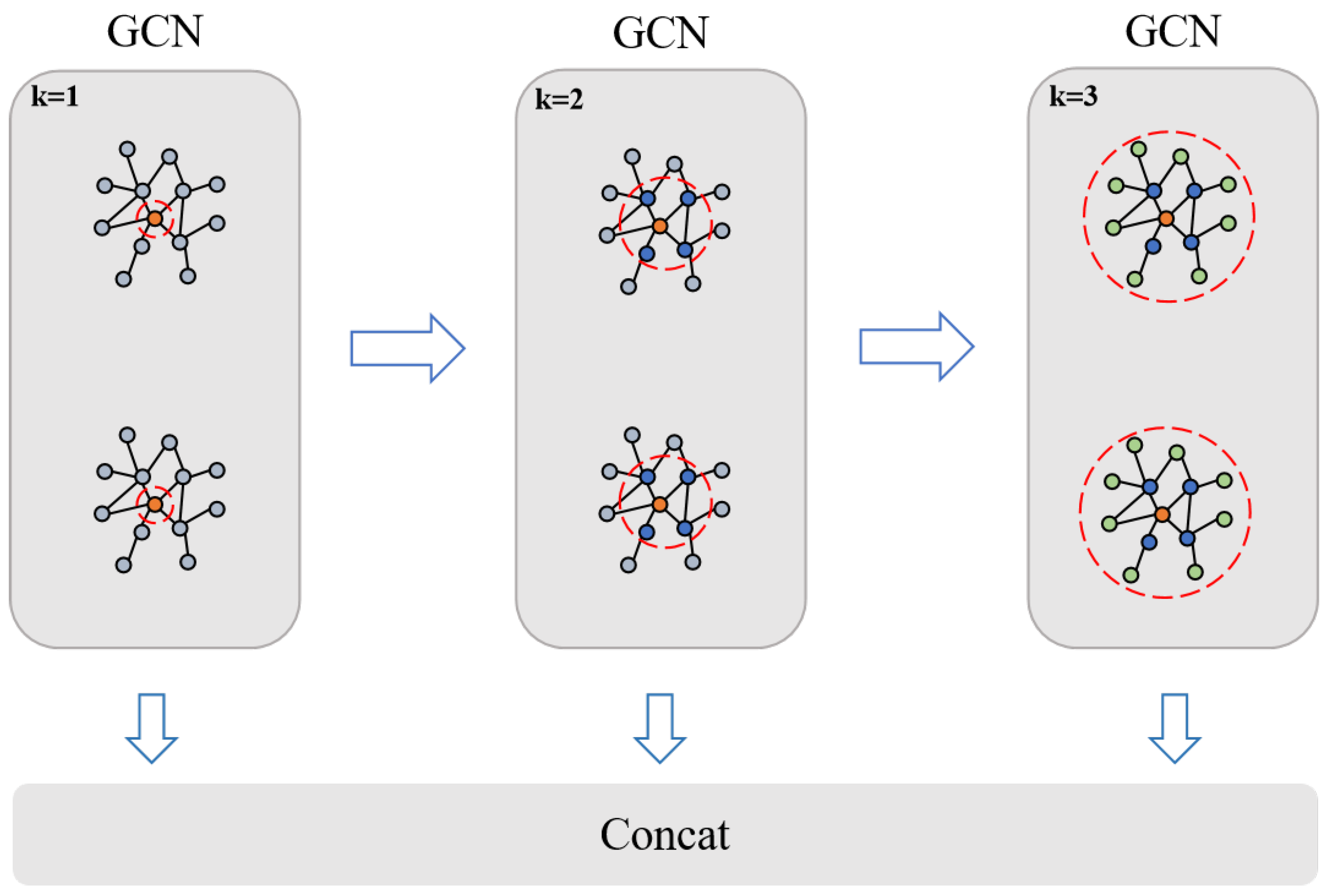
The filter in a graph convolution can be represented by a polynomial of order K, and the parameter K is also referred to as the kernel size of the graph convolution. When utilizing Chebyshev polynomials to approximate the filter, its order remains fixed. This implies that the receptive field of the graph convolution layer is also fixed, limiting its ability to learn multi-domain information. To address this limitation and aggregate information from different receptive fields, a multi-perceptual graph convolution neural network (MPGCN) is designed.
The specific structure of the MPGCN is illustrated in Figure 5. The MPGCN comprises three GConv layers with varying receptive fields designed to capture the characteristics of the instance graph. The key idea of the MPGCN is to collect information from different receptive fields and combine features through the concat layer, aiming to create a more robust feature representation. It consists of three parallel graph convolution layers with different receptive fields (k = 1, k = 2, k = 3), which can perceive the information of different numbers of neighbors.
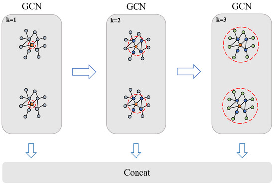
Figure 5.
MPGCN structure diagram.
Features from these neighborhoods are then computed to fuse the output features into enhanced feature representations. For a graph with node feature , its convolution with the GConv layer can be defined as follows:
where , , and represent the size of the receiving field, A is the constructed adjacency matrix, X is the node characteristic matrix, and , , and denote the weight matrix of each receptive field. Therefore, the feature representation learned by the MPGCN for the input graph can be defined as follows:
where , , and are the learned features from the first, second, and third GConv, and W is the trainable weight matrix.
3.3. Domain Discrimination Module
3.3.1. Fault Classifier
Fault classifiers are used to identify the health status of bearings, so it is necessary to distinguish the type of fault of the input sample. Cross-entropy loss is selected to evaluate classification errors between the results of the true label and the classification results. The classification loss function is as follows:
where is the mathematical expectation, represents the cross-entropy loss, and represents the i-th output of the sample in the source domain.
3.3.2. Domain Discriminator
Due to domain shift issues, models trained solely on samples from the source domain often do not yield optimal diagnostic results when applied directly to samples from the target domain. To address this problem, this module incorporates a domain discriminator designed to differentiate which domain the extracted features originate from. Binary cross-entropy loss is chosen as the adversarial domain classifier. The adversarial loss for an input sample can be calculated as follows:
where represents the real domain label, and represents the predicted domain label for that sample. Therefore, the adversarial loss for all samples can be calculated as follows:
where and denote the features learned from the source domain and the target domain, and and , respectively, denote the sample size input between the two domains.
3.3.3. Total Loss Function
In the model training process, the parameters of each part of the model are updated using the backpropagation algorithm (BP), which is expressed by combining the above loss function. The proposed method’s overall loss function has the following expression:
where the parameter represents the tradeoff parameter.
The parameters , , and represent the parameters of the MPGCN F, the fault classifier C, and the domain discriminator D, respectively. The parameters are updated as follows:
It is possible to acquire domain-invariant and discriminative features by optimizing the MPGCTN parameters and minimizing the given overall objective function. This enables accurate classification of data from unlabeled target domains by the classifier trained on labeled source domain data. Therefore, the algorithm created by using the proposed MPGCTN for domain adaptation is summarized in Algorithm 1.
| Algorithm 1: Multi-perception graph convolution transfer network for domain adaptation. | |
| Input: Source domain sample | |
| Target domain sample | |
| Output: Trained classifier C | |
| Trained MPGCN F | |
| Trained Domain Discriminator D | |
| for number of epoches do | |
| 1. Generate the source graphs | |
| 2. Generate the target graphs | |
| 3. Extract source features: | |
| 4. Extract target features: | |
| 5. Compute adversarial loss | |
| 6. Compute classification loss | |
| 7. Compute total loss | |
| 8. Update by loss | |
| end | |
4. Experimental Verification and Analysis
The diagnostic performance of this method under variable working conditions is verified by contrast experiments with bearing datasets from Case Western Reserve University (CWRU) and Paderborn University (PU).
4.1. Experiment I
4.1.1. Dataset Description
The bearing dataset used in the first experiment is obtained from Case Western Reserve University (CWRU) [12]. The test bench of the CWRU dataset is shown in Figure 6. The bearing dataset was collected by an acceleration sensor at four different loads (0HP, 1HP, 2HP, and 3HP) corresponding to four different rotational speeds. The dataset is divided into four states: normal condition (N), inner race failure (IF), outer race failure (OF), and rolling body failure (RF). At the same time, corresponding to each type of fault, there are three different damage diameters on the bearing, 0.007 inch, 0.014 inch, and 0.021 inch, a total of 10 fault types. Specific bearing damage information is shown in Table 1.
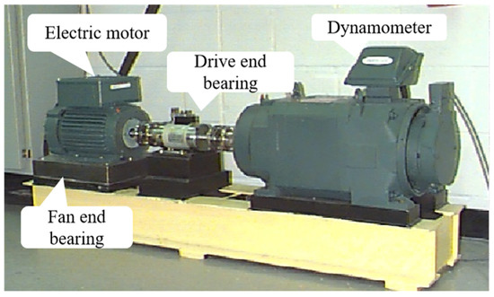
Figure 6.
Bearing failure simulation test bench from CWRU.

Table 1.
Bearing damage information from CWRU dataset.
4.1.2. Experimental Settings
In this experiment, the input sample length is divided into 1024. The dataset consists of 300 examples from each category for a total of 3000 samples. The ratio of samples is set to 70% for training and 30% for testing. To be exact, training is carried out using 2100 labeled source domain samples, and testing is carried out with 900 unlabeled target domain samples and 900 unlabeled target operating condition samples. Additionally, the dataset includes different operating conditions denoted as 0, 1, 2, and 3, as shown in Table 2. In the experiment, 12 transfer tasks are configured under these four working situations. In order to set transfer tasks under different working conditions, is used to represent that the source domain is the data collected under the working condition a, and the target domain is the transfer task with the data collected under the working condition b.
Table 2.
Data corresponding to different working conditions.
In order to ensure the convergence of the model, the learning rate is configured to decay with loss. For each training iteration, the training data batch size is set to 128 with an Adam optimizer and 100 rounds of training per model. In addition, all methods are trained under the PyTorch framework using a GPU model of NVIDIA GTX4060 ti (Asus, Shanghai, China).
4.1.3. Analysis of Experimental Results
To demonstrate the effectiveness of the proposed model, six models are applied for validation comparison. They are Baseline [25], maximum mean discrepancy (MMD) [26], multi kernel maximum mean discrepancy (MKMMD) [27], correlation alignment (CORAL) [28], domain adversarial neural networks (DANNs) [29], adversarial discriminative domain adaptation (ADDA) [30], and the proposed MPGCTN. Each transfer learning method adopts the same feature extraction network and configuration of the training set and test set to verify the advantages of this method. A feature extraction network is employed to generate a Baseline for direct transfer. The diagnosis accuracy metric is the most important for this investigation. The average of ten experiments is utilized as the outcome to reduce the effect of chance on the results.
The experimental results are listed in Table 3. Table 3 shows that, for each transfer task, the approach suggested in this study can produce the highest diagnostic accuracy. This method not only has higher precision, but also has smaller mean difference, which is better than other methods. In addition, on the most difficult task , the diagnosis result of the worst-performing method is 89.83%, while the diagnosis result of the proposed MPGCTN method is 99.64%, an improvement of 9.81%.
Table 3.
Diagnostic accuracy of CWRU datasets.
The results show that the proposed method combines a graph convolutional network with an adversarial domain adaptation and can extract more data features so as to obtain the best diagnostic results. It is confirmed that the proposed MPGCTN is superior in diagnosing bearing faults in varying operating situations.
4.2. Experiment II
4.2.1. Description of the Dataset
In order to further verify the applicability of the proposed model, the proposed method is applied to an actual damage dataset. The rolling bearing dataset used in Experiment II comes from Paderborn University (PU) and includes two types of bearing failure data: simulated machining damage data and actual bearing damage data [31].
The experiment utilizes real damage data from ball bearings collected during accelerated life tests. The PU accelerated life test rig is depicted in Figure 7, comprising a bearing housing and an electric motor that drives a shaft containing four test bearings. In the PU dataset, the speed of the drive system, load torque, and radial load vary, and corresponding bearing vibration data are collected under four different operating conditions. The specific parameters for each condition are detailed in Table 4. In addition, the data collected under each condition include 13 different fault categories, and Table 5 provides information on the actual failure categories in the accelerated life tests conducted in this dataset.
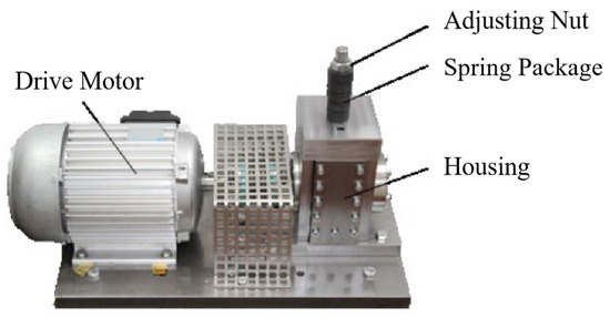
Figure 7.
Accelerated life test rig from PU.
Table 4.
Working condition information from PU dataset.
Table 5.
Real damage bearing fault category in PU dataset.
4.2.2. Experimental Settings
The sample length used in this example is 1024. There are 3900 samples in total in the dataset, 300 samples for each fault type (a total of 13 fault categories). Of the samples, 70% are used as the training set and 30% as the testing set. is used to represent the transfer task from working condition a to working condition b in this experiment. In order to better reflect the generalization ability of the model, the diagnostic model parameters used in this experiment are consistent with Experiment I. Baseline, MMD, MKMMD, CORAL, DANN, and ADDA are selected as comparison models to demonstrate the MPGCTN’s performance. The feature mining network is also used as a Baseline for direct transfer.
4.2.3. Analysis of Experimental Results
The experimental results of the PU bearing data are shown in Table 6. It can be seen that the MPGCTN can achieve the best diagnostic effect in each task. In addition, on the most difficult task , the highest diagnostic accuracy of the contrast model is 43.05%, while that of the proposed MPGCTN method is 68.12%, an increase of 25.07%.
Table 6.
Diagnostic accuracy of PU dataset.
At the same time, it can be seen that some of the comparison models can obtain good results in some tasks, but their diagnostic performance is not stable enough in other tasks, which verifies that the proposed MPGCTN method has good generalization. Based on the above results, it is verified that the proposed method has excellent diagnostic performance in the actual damaged bearing dataset.
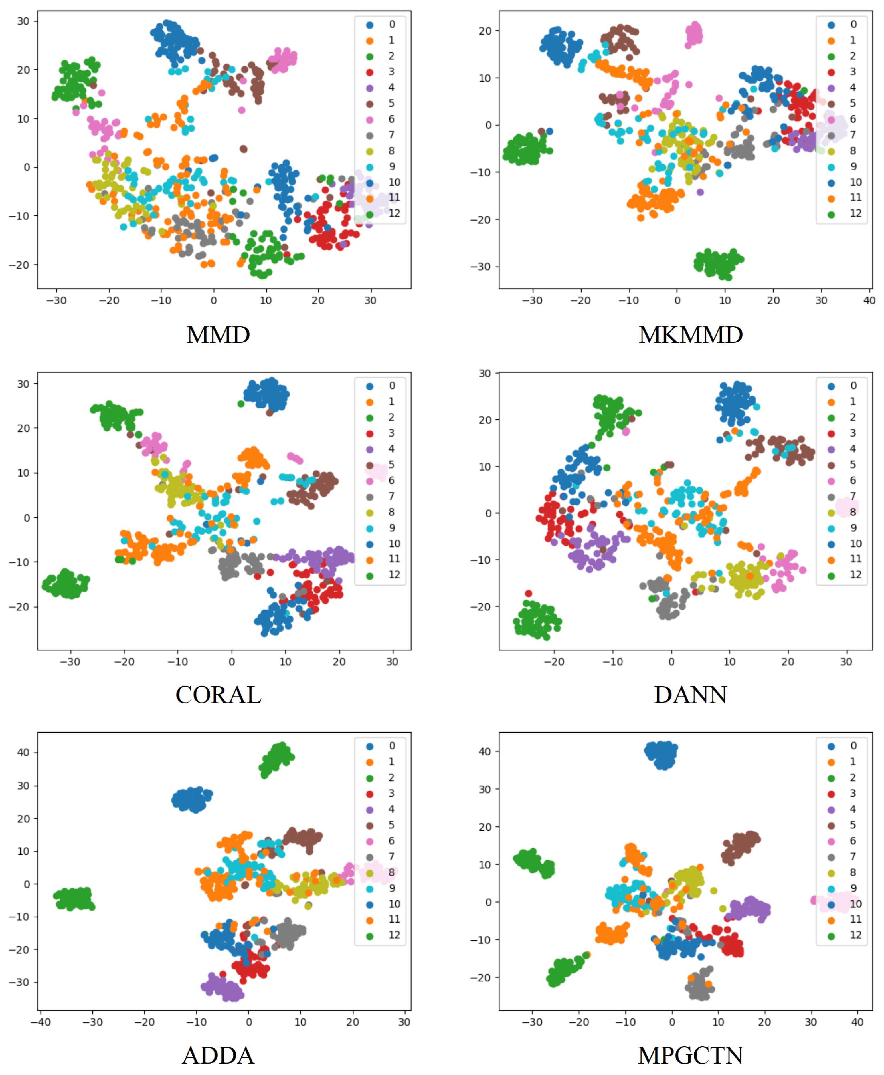
In order to further verify the transfer performance of the designed method, t-distributed stochastic neighbor embedding (t-SNE) [32] is used to map the learned high-dimensional features to the two-dimensional space to effectively demonstrate the advantages of the MPGCTN. The t-SNE diagrams generated for the task using the six models are shown in Figure 8. It shows the feature distributions learned by MMD, MKMMD, CORAL, DANN, ADDA, and the MPGCTN after training. From the visualization results of the six models, it can be seen that, although the classification visualization results of the MKMMD and CORAL distinguish most categories, there are still some classification errors that lead to overlap. The experimental results show that, compared with MKMMD and CORAL, the proposed MPGCTN can capture more domain-sharing discriminant features.
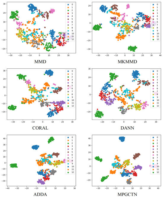
Figure 8.
Comparison of t-SNE visualization results.
The visualization results show that the ADDA based on adversarial strategy has a better classification effect, second only to the proposed MPGCTN. It shows that the proposed MPGCTN can mine more data information, which helps achieve better classification. The overlap between different classes is minimal, and the same classes have good clustering. This is because the MPGCTN method, supported by the MPGCN, reduces the probability of sample classification errors at each class boundary by modeling the input data structure at multiple scales. The comparison results clearly show that the MPGCTN has better transfer performance than other transfer learning methods.
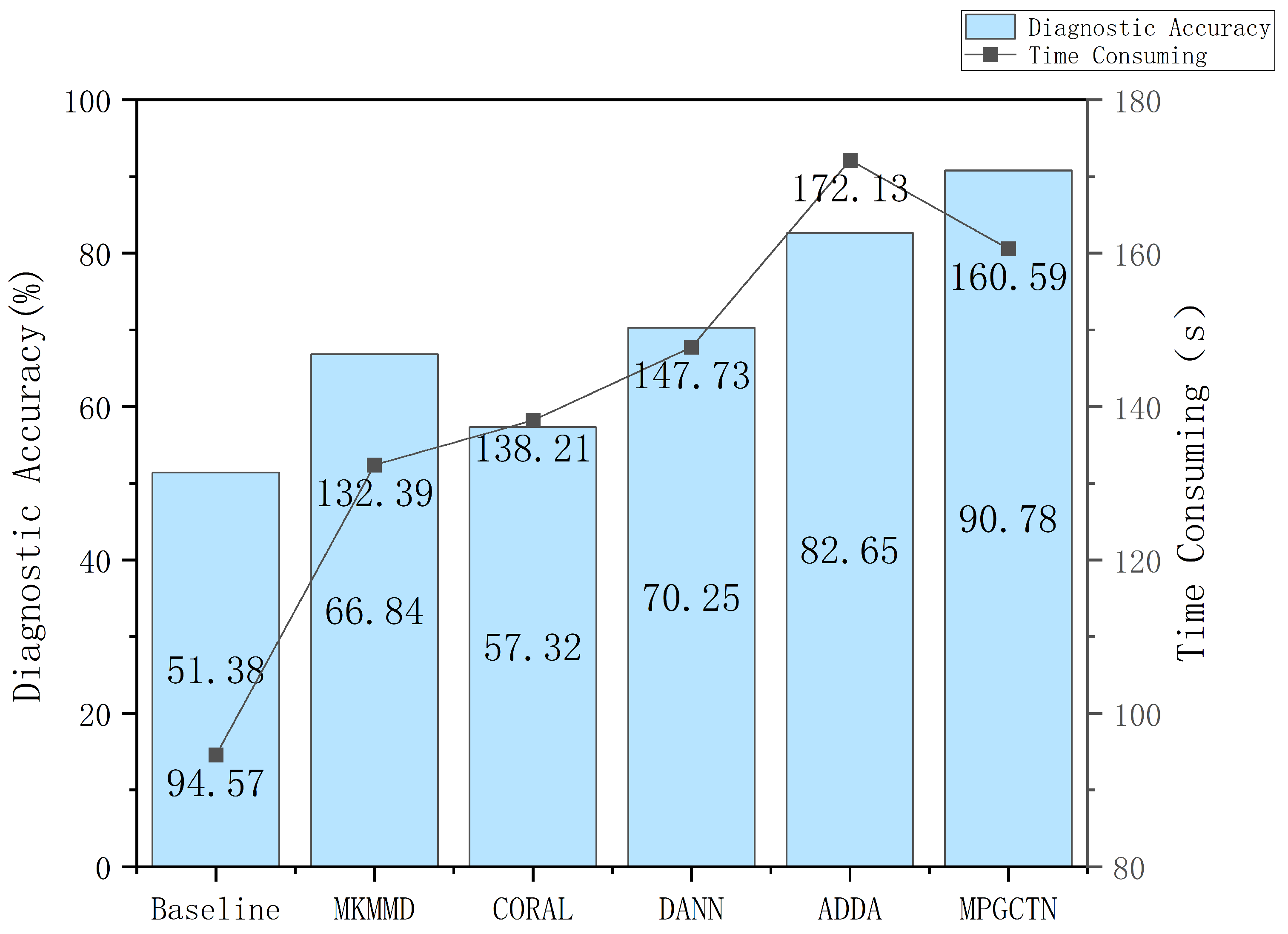
In addition to the above experiments, we also consider the computational efficiency of the proposed method in practical applications. The time consumption and diagnostic accuracy of the MPGCTN are compared with other methods on task , as shown in Figure 9. As you can see from the figure, ADDA takes the most time. Compared with other methods, the time taken by the proposed method is not long, but the diagnosis effect is the best. The results show that the proposed MPGCTN can improve the diagnostic accuracy without high time consumption.
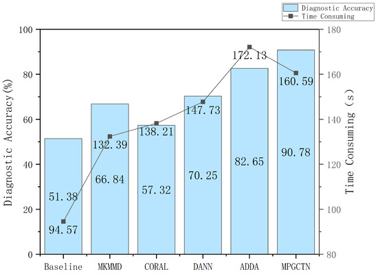
Figure 9.
Comparison of time consumption and diagnostic accuracy of MPGCTN with other methods.
4.3. Ablation Experiment
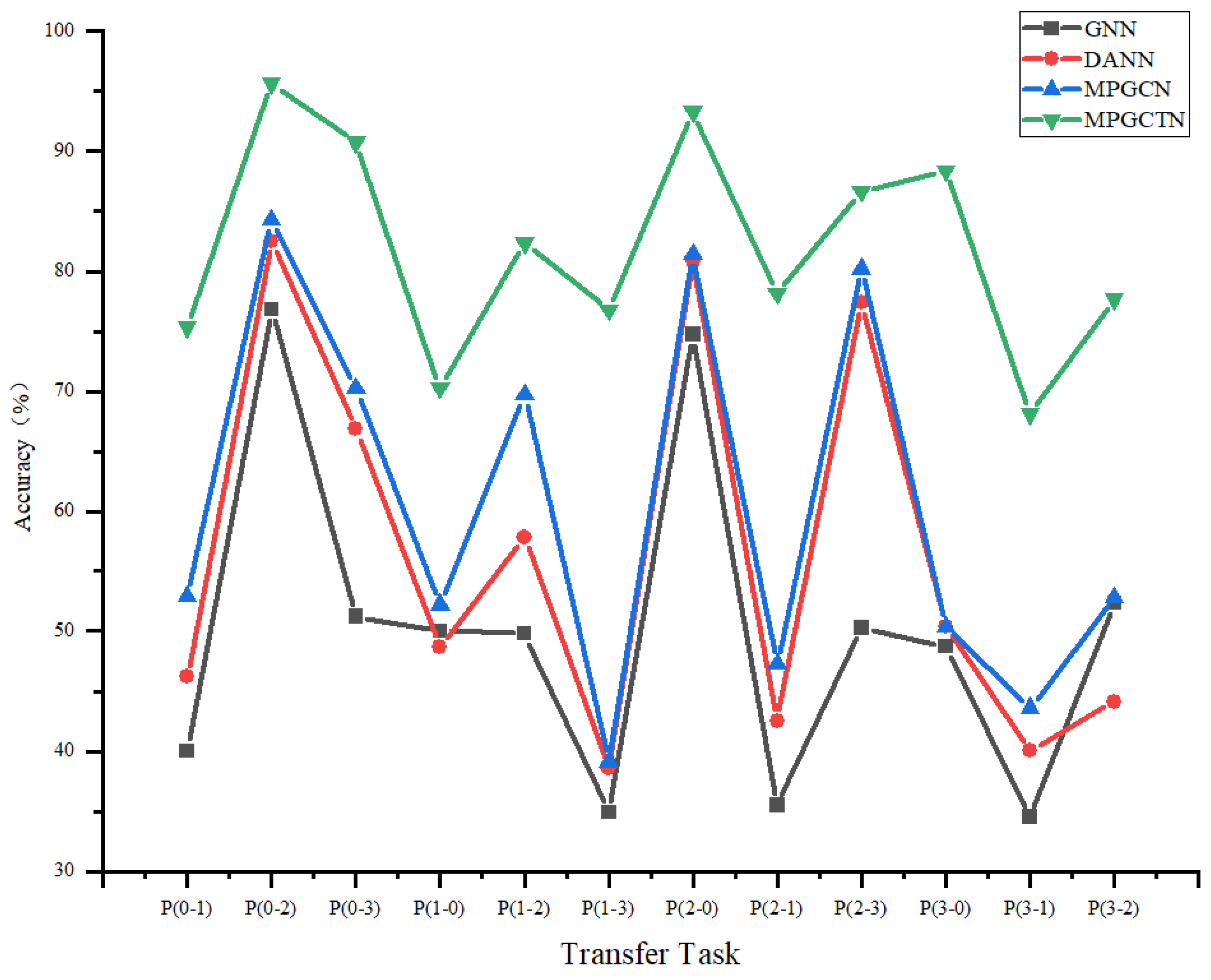
To find the influence of each module on the performance of the model, an ablation experiment is used to evaluate the impact of the graph perception module and the domain discrimination module on the performance of fault diagnosis. Three models, the GNN, DANN, and MPGCN, are set up as controls. Results of the ablation experiment are shown in Figure 10.
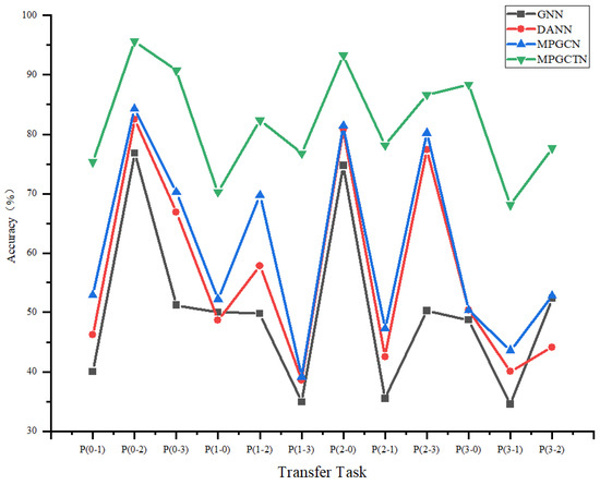
Figure 10.
Comparison of t-SNE visualization results.
The comparison reveals that the incorporation of both the graph generation module and the graph perception module significantly enhances the diagnostic performance of the proposed method.
5. Conclusions
In this paper, a novel graph convolutional network is designed to extract multi-scale structural features, and an MPGCTN is proposed for bearing fault diagnosis. The three modules in the MPGCTN can realize the modeling of sample class labels, domain labels, and data structures so as to complete high-precision cross-domain diagnosis. The experimental results of two cases show that the classification accuracy of the MPGCTN is higher than that of other methods. However, some issues remain unresolved:
(1) This paper ignores the influence of the interpretability of graph neural networks. We cannot fully explain this model;
(2) The ability of the model to transfer diagnostic generalization between different devices is unexplored.
In order to enhance diagnostic performance, we will take these two issues into account in later research and create appropriate solutions.
Author Contributions
X.P.: Conceptualization, Methodology, Writing—original draft, and Funding acquisition. H.C.: Methodology, Software and Validation. D.Z.: Formal analysis, Validation, and Writing—review and editing. A.S.: Investigation, Validation, and Writing—review and editing. X.S.: Writing—review and editing. All authors have read and agreed to the published version of the manuscript.
Funding
This research was funded by the Shanghai Sailing Program under Grant No. 20YF1414800, and Shanghai Rising-Star Program under Grant No. 21QA1403400.
Institutional Review Board Statement
Not applicable.
Informed Consent Statement
Not applicable.
Data Availability Statement
The raw data are contained within the article.
Conflicts of Interest
The authors declare no conflicts of interest.
References
- Zhao, Z.; Zhang, Q.; Yu, X.; Sun, C.; Wang, S.; Yan, R.; Chen, X. Applications of Unsupervised Deep Transfer Learning to Intelligent Fault Diagnosis: A Survey and Comparative Study. IEEE Trans. Instrum. Meas. 2021, 70, 1–28. [Google Scholar] [CrossRef]
- Zhao, Z.; Jiao, Y. A Fault Diagnosis Method for Rotating Machinery Based on CNN with Mixed Information. IEEE Trans. Ind. Informat. 2023, 19, 9091–9101. [Google Scholar] [CrossRef]
- Zhang, W.; Peng, G.; Li, C.; Chen, Y.; Zhang, Z. A New Deep Learning Model for Fault Diagnosis with Good Anti-Noise and Domain Adaptation Ability on Raw Vibration Signals. Sensors 2017, 17, 425. [Google Scholar] [CrossRef] [PubMed]
- Hu, Y.; Liu, R.; Li, X.; Chen, D.; Hu, Q. Task-Sequencing Meta Learning for Intelligent Few-Shot Fault Diagnosis with Limited Data. IEEE Trans. Ind. Inform. 2022, 18, 3894–3904. [Google Scholar] [CrossRef]
- Khoukhi, A.; Khalid, M.H. Hybrid Computing Techniques for Fault Detection and Isolation, a Review. Comput. Electr. Eng. 2015, 43, 17–32. [Google Scholar] [CrossRef]
- Wu, H.; Li, J.; Zhang, Q.; Tao, J.; Meng, Z. Intelligent Fault Diagnosis of Rolling Bearings under Varying Operating Conditions Based on Domain-Adversarial Neural Network and Attention Mechanism. ISA Trans. 2022, 130, 477–489. [Google Scholar] [CrossRef] [PubMed]
- Inayat, U.; Zia, M.F.; Mahmood, S.; Khalid, H.M.; Benbouzid, M. Learning-Based Methods for Cyber Attacks Detection in IoT Systems: A Survey on Methods, Analysis, and Future Prospects. Electronics 2022, 11, 1502. [Google Scholar] [CrossRef]
- Siddique, M.F.; Ahmad, Z.; Ullah, N.; Kim, J. A Hybrid Deep Learning Approach: Integrating Short-Time Fourier Transform and Continuous Wavelet Transform for Improved Pipeline Leak Detection. Sensors 2023, 23, 8079. [Google Scholar] [CrossRef] [PubMed]
- Guo, X.; Chen, L.; Shen, C. Hierarchical Adaptive Deep Convolution Neural Network and Its Application to Bearing Fault Diagnosis. Measurement 2016, 93, 490–502. [Google Scholar] [CrossRef]
- Ullah, N.; Ahmad, Z.; Siddique, M.F.; Im, K.; Shon, D.K.; Yoon, T.H.; Yoo, D.S.; Kim, J.M. An Intelligent Framework for Fault Diagnosis of Centrifugal Pump Leveraging Wavelet Coherence Analysis and Deep Learning. Sensors 2023, 23, 8850. [Google Scholar] [CrossRef]
- Gao, J.; Wang, H.; Shen, H. Task Failure Prediction in Cloud Data Centers Using Deep Learning. IEEE Trans. Serv. Comput. 2022, 15, 1411–1422. [Google Scholar] [CrossRef]
- Chen, X.; Yang, R.; Xue, Y.; Huang, M.; Ferrero, R.; Wang, Z. Deep Transfer Learning for Bearing Fault Diagnosis: A Systematic Review Since 2016. IEEE Trans. Instrum. Meas. 2023, 72, 3508221. [Google Scholar] [CrossRef]
- Huo, C.; Jiang, Q.; Shen, Y.; Zhu, Q.; Zhang, Q. Enhanced Transfer Learning Method for Rolling Bearing Fault Diagnosis Based on Linear Superposition Network. Eng. Appl. Artif. Intell. 2023, 121. [Google Scholar] [CrossRef]
- Li, X.; Zhang, W.; Ma, H.; Luo, Z.; Li, X. Partial Transfer Learning in Machinery Cross-Domain Fault Diagnostics Using Class-Weighted Adversarial Networks. Neural Netw. 2020, 129, 313–322. [Google Scholar] [CrossRef] [PubMed]
- Huang, M. A Fault Diagnosis Method of Bearings Based on Deep Transfer Learning. Simul. Modell. Pract. Theory 2023, 122, 102659. [Google Scholar] [CrossRef]
- Jiao, J.; Zhao, M.; Lin, J. Unsupervised Adversarial Adaptation Network for Intelligent Fault Diagnosis. IEEE Trans. Ind. Electron. 2020, 67, 9904–9913. [Google Scholar] [CrossRef]
- Kuang, J.; Xu, G.; Tao, T.; Wu, Q. Class-Imbalance Adversarial Transfer Learning Network for Cross-Domain Fault Diagnosis with Imbalanced Data. IEEE Trans. Instrum. Meas. 2022, 71, 1–11. [Google Scholar] [CrossRef]
- Wan, L.; Li, Y.; Chen, K.; Gong, K.; Li, C. A Novel Deep Convolution Multi-Adversarial Domain Adaptation Model for Rolling Bearing Fault Diagnosis. Measurement 2022, 191, 110752. [Google Scholar] [CrossRef]
- Chen, Z.; Xu, J.; Alippi, C.; Ding, S.X.; Shardt, Y.; Peng, T.; Yang, C. Graph Neural Network-Based Fault Diagnosis: A Review. arXiv 2021, arXiv:2111.08185. [Google Scholar]
- Defferrard, M.; Bresson, X.; Vandergheynst, P. Convolutional Neural Networks on Graphs with Fast Localized Spectral Filtering. In Proceedings of the 30th Conference on Neural Information Processing Systems (NIPS 2016), Barcelona, Spain, 5–10 December 2016; Volume 29. [Google Scholar]
- Tang, H.; Chen, K.; Jia, K. Unsupervised Domain Adaptation via Structurally Regularized Deep Clustering. In Proceedings of the IEEE/CVF Conference on Computer Vision and Pattern Recognition, Seattle, WA, USA, 13–19 June 2020; pp. 8725–8735. [Google Scholar]
- HassanPour Zonoozi, M.; Seydi, V. A Survey on Adversarial Domain Adaptation. Neural Process. Lett. 2023, 55, 2429–2469. [Google Scholar] [CrossRef]
- Wu, Y.; Zhao, R.; Ma, H.; He, Q.; Du, S.; Wu, J. Adversarial Domain Adaptation Convolutional Neural Network for Intelligent Recognition of Bearing Faults. Measurement 2022, 195, 111150. [Google Scholar] [CrossRef]
- He, C.; Cao, Y.; Yang, Y.; Liu, Y.; Liu, X.; Cao, Z. Fault Diagnosis of Rotating Machinery Based on the Improved Multidimensional Normalization ResNet. IEEE Trans. Instrum. Meas. 2023, 72, 3524311. [Google Scholar] [CrossRef]
- Kiranyaz, S.; Avci, O.; Abdeljaber, O.; Ince, T.; Gabbouj, M.; Inman, D.J. 1D Convolutional Neural Networks and Applications: A Survey. Mech. Syst. Sig. Process. 2021, 151, 107398. [Google Scholar] [CrossRef]
- Zhang, D.; Ye, M.; Liu, Y.; Xiong, L.; Zhou, L. Multi-Source Unsupervised Domain Adaptation for Object Detection. Inform. Fusion 2022, 78, 138–148. [Google Scholar] [CrossRef]
- Cheng, L.; An, Z.; Guo, Y.; Ren, M.; Yang, Z.; McLoone, S. MMFSL: A Novel Multimodal Few-Shot Learning Framework for Fault Diagnosis of Industrial Bearings. IEEE Trans. Instrum. Meas. 2023, 72, 3525313. [Google Scholar] [CrossRef]
- Wang, H.; Bai, X.; Tan, J.; Yang, J. Deep Prototypical Networks Based Domain Adaptation for Fault Diagnosis. J. Intell. Manuf 2022, 33, 973–983. [Google Scholar] [CrossRef]
- Ganin, Y.; Ustinova, E.; Ajakan, H.; Germain, P.; Larochelle, H.; Laviolette, F.; Marchand, M.; Lempitsky, V. Domain-Adversarial Training of Neural Networks. In Domain Adaptation in Computer Vision Applications; Csurka, G., Ed.; Springer International Publishing: Cham, Switzerland, 2017; pp. 189–209. [Google Scholar]
- Tang, H.; Jia, K. Discriminative Adversarial Domain Adaptation. In Proceedings of the AAAI Conference on Artificial Intelligence, Honolulu, HI, USA, 27 January–1 February 2019; Volume 34, pp. 5940–5947. [Google Scholar]
- Kurmi, V.K.; Namboodiri, V.P. Looking Back at Labels: A Class Based Domain Adaptation Technique. In Proceedings of the 2019 International Joint Conference on Neural Networks (IJCNN), Budapest, Hungary, 14–19 July 2019; pp. 1–8. [Google Scholar]
- van der Maaten, L.; Hinton, G. Visualizing Data Using T-SNE. J. Mach. Learn. Res. 2008, 9, 2579–2605. [Google Scholar]


Disclaimer/Publisher’s Note: The statements, opinions and data contained in all publications are solely those of the individual author(s) and contributor(s) and not of MDPI and/or the editor(s). MDPI and/or the editor(s) disclaim responsibility for any injury to people or property resulting from any ideas, methods, instructions or products referred to in the content. |
© 2024 by the authors. Licensee MDPI, Basel, Switzerland. This article is an open access article distributed under the terms and conditions of the Creative Commons Attribution (CC BY) license (https://creativecommons.org/licenses/by/4.0/).