
Multibody Analysis of Sloshing Effect in a Glass Cylinder Container for Visual Inspection Activities


Abstract
:1. Introduction
2. Materials and Methods
- g = gravitational acceleration;
- R = container radius;
- = static height of the liquid;
- = j-th root of the derivative of the Bessel function of the first kind (for the first fundamental mode, it is equal to 1.841).
- The incompressibility of the liquid;
- A non-viscous flow rate;
- No environmental speed;
- A two-dimensional system;
- Small amplitudes of the wave.
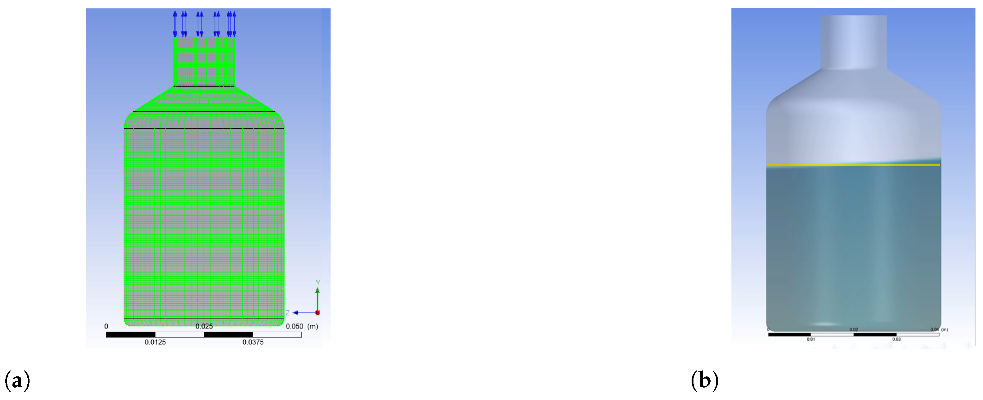
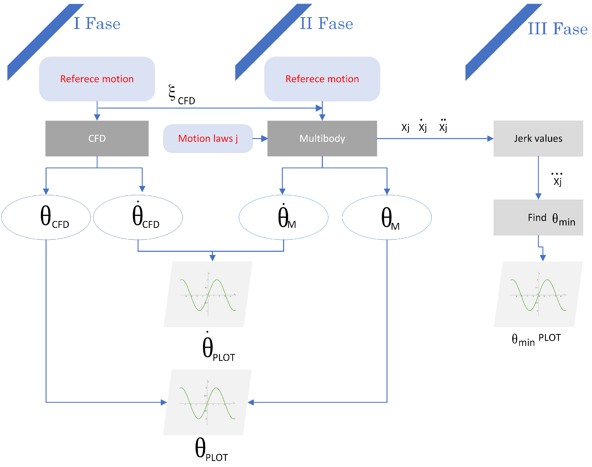
3. Numerical Activity
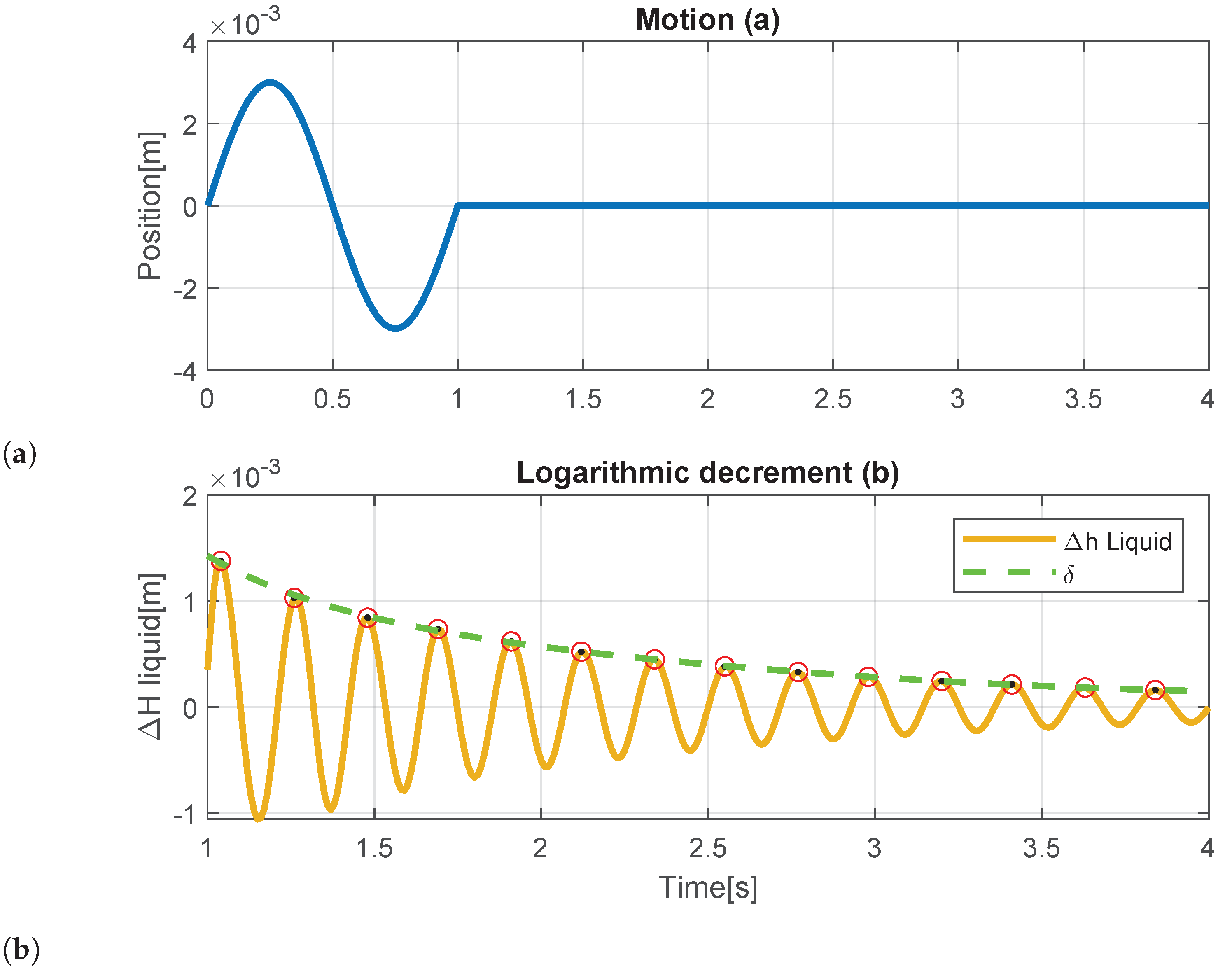
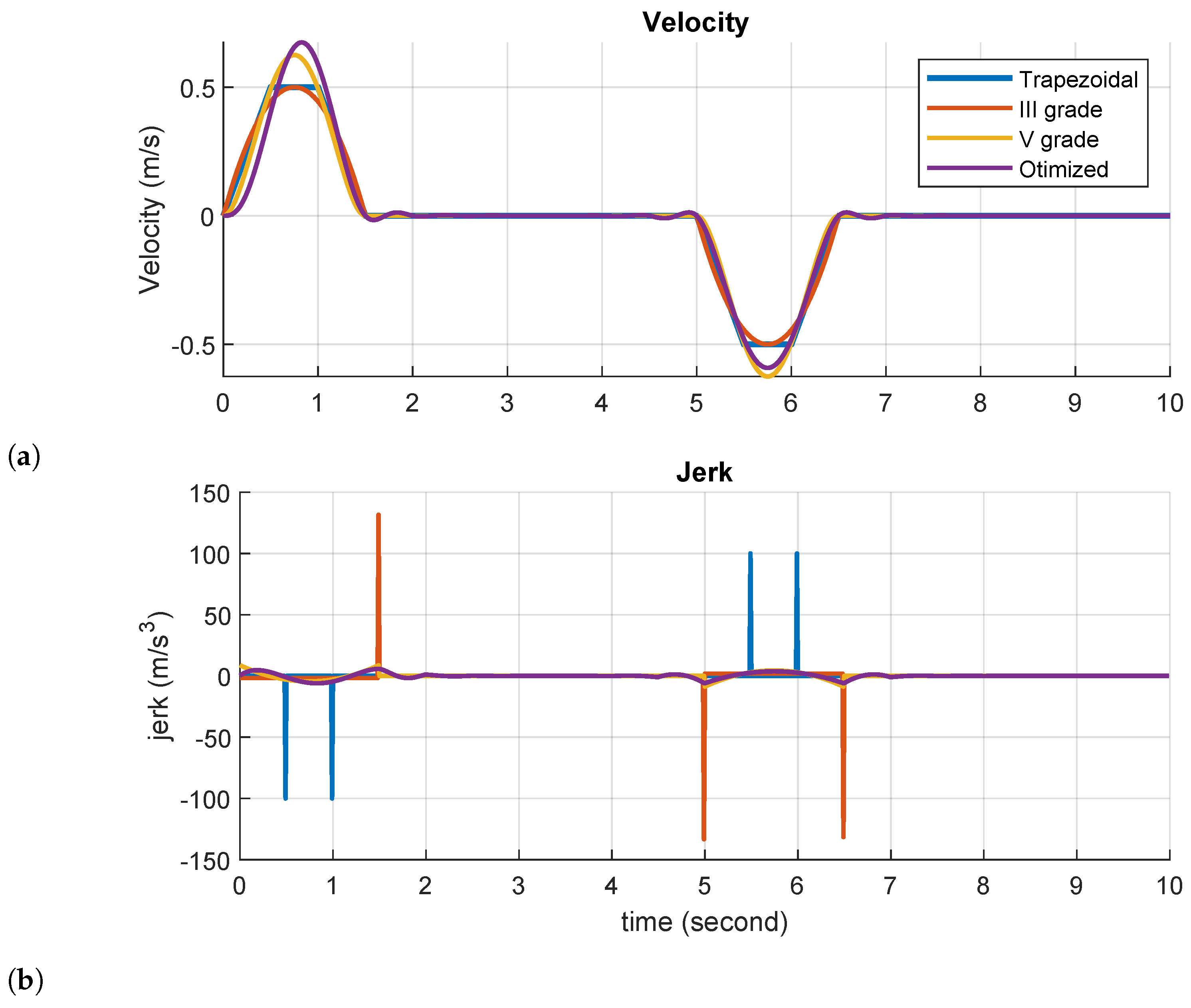
4. Results
5. Conclusions
Author Contributions
Funding
Institutional Review Board Statement
Informed Consent Statement
Data Availability Statement
Conflicts of Interest
References
- Kim, G.; Rhee, H.; Jeon, W.; Jeong, J.; Hwang, D.S. Lateral Sloshing Analysis by CFD and Experiment for a Spherical Tank. Int. J. Aeronaut. Space Sci. 2020, 21, 816–825. [Google Scholar] [CrossRef]
- Orr, J.; Wall, J.; VanZwieten, T.; Hall, C. Space launch system ascent flight control design. In Proceedings of the 2014 American Astronautical Society (AAS) Guidance, Navigation, and Control Conference, Breckenridge, CO, USA, 31 January–5 February 2014; Volume 151, pp. 141–154. [Google Scholar]
- Li, Q.; Ma, X.; Wang, T. Equivalent mechanical model for liquid sloshing during draining. Acta Astronaut. 2011, 68, 91–100. [Google Scholar] [CrossRef]
- Nimisha, P.; Jayalekshmi, B.; Venkataramana, K. Effect of Frequency Content of Seismic Excitation on Slosh Response of Liquid Tank with Baffle Plate. J. Earthq. Tsunami 2023, 17, 2350001. [Google Scholar] [CrossRef]
- Tang, Z.; Sheng, J.; Dong, Y. Effects of tuned liquid dampers on the nonlinear seismic responses of high-rise structures using real-time hybrid simulations. J. Build. Eng. 2023, 70, 106333. [Google Scholar] [CrossRef]
- Ren, H.; Fan, Q.; Lu, Z. Experimental Study and Damping Effect Analysis of a New Tuned Liquid Damper Based on Karman Vortex Street Theory. Buildings 2023, 13, 1013. [Google Scholar] [CrossRef]
- Mei, S.; Liu, M.; Kudreyko, A.; Cattani, P.; Baikov, D.; Villecco, F. Bendlet Transform Based Adaptive Denoising Method for Microsection Images. Entropy 2022, 24, 869. [Google Scholar] [CrossRef] [PubMed]
- Wang, T.; Guercio, V.; Cattani, P.; Villecco, F. A Review of Research Progress and Application of Wavelet Neural Networks. Lect. Notes Netw. Syst. 2023, 687 LNNS, 504–515. [Google Scholar] [CrossRef]
- Christidi-Loumpasefski, O.O.; Rekleitis, G.; Papadopoulos, E.; Ankersen, F. On System Identification of Space Manipulator Systems Including Their Fuel Sloshing Effects. IEEE Robot. Autom. Lett. 2023, 8, 2446–2453. [Google Scholar] [CrossRef]
- Xin, S.; Liang, L.; Wei, S.; Shuyuan, X. A trajectory planning method based on feedforward compensation and quintic polynomial interpolation. In Proceedings of the 2019 14th IEEE International Conference on Electronic Measurement & Instruments (ICEMI), Changsha, China, 1–3 November 2019; pp. 434–441. [Google Scholar] [CrossRef]
- Sharma, D.; Dhiman, C.; Kumar, D. Evolution of visual data captioning Methods, Datasets, and evaluation Metrics: A comprehensive survey. Expert Syst. Appl. 2023, 221. [Google Scholar] [CrossRef]
- Manca, A.G.; Pappalardo, C.M. Topology optimization procedure of aircraft mechanical components based on computer-aided design, multibody dynamics, and finite element analysis. Lect. Notes Mech. Eng. 2020, 2, 159–168. [Google Scholar] [CrossRef]
- De Simone, M.; Veneziano, S.; Guida, D. Design of a Non-Back-Drivable Screw Jack Mechanism for the Hitch Lifting Arms of Electric-Powered Tractors. Actuators 2022, 11, 358. [Google Scholar] [CrossRef]
- Pappalardo, C.M.; De Simone, M.C.; Guida, D. Multibody modeling and nonlinear control of the pantograph/catenary system. Arch. Appl. Mech. 2019, 89, 1589–1626. [Google Scholar] [CrossRef]
- De Simone, M.C.; Guida, D. Modal coupling in presence of dry friction. Machines 2018, 6, 8. [Google Scholar] [CrossRef]
- Rivera, Z.B.; De Simone, M.C.; Guida, D. Unmanned ground vehicle modelling in Gazebo/ROS-based environments. Machines 2019, 7, 42. [Google Scholar] [CrossRef]
- Shang, J.; Guan, D. Improvement of damping factors of ITD identification using GLS. Qinghua Daxue Xuebao/Journal Tsinghua Univ. 1997, 37, 46–48. [Google Scholar]
- Kolev, N.I.; Kolev, N.I. Multiphase Flow Dynamics: Fundamentals; Springer: Berlin/Heidelberg, Germany, 2005; Volume 1. [Google Scholar]
- Ibrahim, R.A. Liquid Sloshing Dynamics: Theory and Applications; Cambridge University Press: Cambridge, UK, 2005. [Google Scholar]
- Moriello, L.; Biagiotti, L.; Melchiorri, C.; Paoli, A. Manipulating liquids with robots: A sloshing-free solution. Control. Eng. Pract. 2018, 78, 129–141. [Google Scholar] [CrossRef]
- Gattringer, H.; Müller, A.; Weitzhofer, S.; Schörgenhumer, M. Point to point time optimal handling of unmounted rigid objects and liquid-filled containers. Mech. Mach. Theory 2023, 184, 105286. [Google Scholar] [CrossRef]
- Nan, M.; Junfeng, L.; Tianshu, W. Equivalent mechanical model of large-amplitude liquid sloshing under time-dependent lateral excitations in low-gravity conditions. J. Sound Vib. 2017, 386, 421–432. [Google Scholar] [CrossRef]
- Gangadharan, S.; Sudermann, J.; Marlowe, A.; Njenga, C. Parameter estimation of spacecraft fuel slosh model. In Proceedings of the 45th AIAA/ASME/ASCE/AHS/ASC Structures, Structural Dynamics & Materials Conference, Palm Springs, CA, USA, 19–22 April 2004; Volume 6, pp. 4779–4789. [Google Scholar]
- Liguori, A.; Formato, A.; Pellegrino, A.; Villecco, F. Study of tank containers for foodstuffs. Machines 2021, 9, 44. [Google Scholar] [CrossRef]
- Pappalardo, C.M.; Lök, Ş.İ.; Malgaca, L.; Guida, D. Experimental modal analysis of a single-link flexible robotic manipulator with curved geometry using applied system identification methods. Mech. Syst. Signal Process. 2023, 200, 110629. [Google Scholar] [CrossRef]
- Lök, Ş.İ.; Pappalardo, C.M.; La Regina, R.; Malgaca, L. System Identification of a Nonlinear One-Degree-of-Freedom Vibrating System. Lect. Notes Netw. Syst. 2023, 687, 348–355. [Google Scholar] [CrossRef]
- Gattringer, H.; Mueller, A.; Oberherber, M.; Kaserer, D. Time-optimal robotic manipulation on a predefined path of loosely placed objects: Modeling and experiment. Mechatronics 2022, 84, 102753. [Google Scholar] [CrossRef]
- Cammarata, A.; Maddìo, P.D.; Sinatra, R. Interface reduction in flexible multibody systems. Mater. Res. Proc. 2023, 26, 653–658. [Google Scholar] [CrossRef]
- Li, T.; Kou, Z.; Wu, J.; Yahya, W.; Villecco, F. Multipoint Optimal Minimum Entropy Deconvolution Adjusted for Automatic Fault Diagnosis of Hoist Bearing. Shock Vib. 2021, 2021, 6614633. [Google Scholar] [CrossRef]
- Luo, M.; Xue, M.A.; Yuan, X.; Zhang, F.; Xu, Z. Experimental and Numerical Study of Stratified Sloshing in a Tank under Horizontal Excitation. Shock Vib. 2021, 2021, 6639223. [Google Scholar] [CrossRef]
- Hirt, C.W.; Nichols, B.D. Volume of fluid (VOF) method for the dynamics of free boundaries. J. Comput. Phys. 1981, 39, 201–225. [Google Scholar] [CrossRef]


| Water | Air | ||
|---|---|---|---|
| Properties | Values | Properties | Values |
| Density () | Density () | ||
| Ref. temperature (t) | Ref. temperature (t) | ||
| Ref. pressure (p) | Ref. pressure (p) | ||
| Dynamic viscosity () | Dynamic viscosity () | ||
| CFD Simulation Parameters | ||
| Total time duration | 4 [s] | |
| Time steps | 0.01 [s] | |
| Domains’ Characteristics | ||
| Default domain | Multiphase | Homogeneous model |
| Default domain | Fluid | Air–water |
| Open domain | Boundary type | Opening |
| Open domain | Fluid values | Air = 1; water = 0 |
| Wall domain | Boundary type | Wall |
| Wall domain | Mass and momentum | No slip wall |
| Global initialization | Relative pressure | No slip wall |
| Solver Control | ||
| Advection scheme | High resolution | |
| Transient scheme | Second-order backward Euler | |
| Convergence control | Min. coeff. Loops 1; Max. coeff. Loops 40 | |
| Convergence criteria | Residual type | RMS |
| Convergence criteria | Residual target | 0.0001 |
| Parameters | Expressions | Values |
|---|---|---|
| Liquid density (water) | 1000 | |
| Damping rate for first mode * | 1.841 | |
| Free-surface height | H | 0.039 m |
| Flask radius | r | 0.0205 m |
| Natural pulsation, | 29.7 rad/s | |
| Stiffness coefficient, k | 11.3 N/m | |
| Damping coefficient, | 0.023 Ns/m | |
| Slosh mass, | 0.0132 kg | |
| Pendulum length, | 0.011 m | |
| Pendulum hinge location, | −0.0015 m |
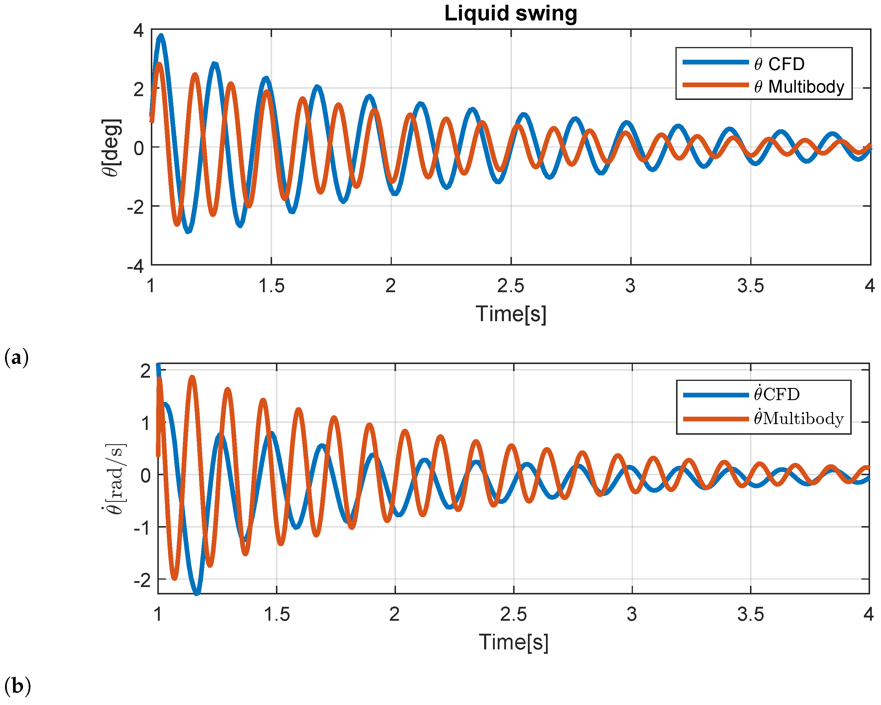
| Parameters | CFD | Multibody |
|---|---|---|
| 28.56 rad/s | 29.7 rad/s | |
| 4.55 Hz | 4.76 Hz | |
| 0.03 | 0.03 |
Disclaimer/Publisher’s Note: The statements, opinions and data contained in all publications are solely those of the individual author(s) and contributor(s) and not of MDPI and/or the editor(s). MDPI and/or the editor(s) disclaim responsibility for any injury to people or property resulting from any ideas, methods, instructions or products referred to in the content. |
© 2024 by the authors. Licensee MDPI, Basel, Switzerland. This article is an open access article distributed under the terms and conditions of the Creative Commons Attribution (CC BY) license (https://creativecommons.org/licenses/by/4.0/).
Share and Cite
De Simone, M.C.; Veneziano, S.; Pace, R.; Guida, D. Multibody Analysis of Sloshing Effect in a Glass Cylinder Container for Visual Inspection Activities. Appl. Sci. 2024, 14, 4522. https://doi.org/10.3390/app14114522
De Simone MC, Veneziano S, Pace R, Guida D. Multibody Analysis of Sloshing Effect in a Glass Cylinder Container for Visual Inspection Activities. Applied Sciences. 2024; 14(11):4522. https://doi.org/10.3390/app14114522
Chicago/Turabian StyleDe Simone, Marco Claudio, Salvio Veneziano, Raffaele Pace, and Domenico Guida. 2024. "Multibody Analysis of Sloshing Effect in a Glass Cylinder Container for Visual Inspection Activities" Applied Sciences 14, no. 11: 4522. https://doi.org/10.3390/app14114522