Analyzing Temperature Distributions and Gradient Behaviors for Early-Stage Tumor Lesions in 3D Computational Model of Breast

Abstract

The computational modelling and analysis of internal and external temperature distributions and their gradients, associated with the first stage of mammary tumors, was performed to relate thermal parameters to relevant tumor characteristics. A realistic 3D geometric model of breast anatomy was used to simulate tumor cases that were characterized in real life at their primary clinical stage. The thermophysical parameters of three tumors were extracted to implement the models; a fourth case without a tumor was used as a reference to provide quantitative measurements of temperature increases and gradient changes. The analysis considered superficial and internal temperature distributions and gradients, computed throughout specific paths. Finally, an evaluation was made of the ability of the thermometric technologies available today to detect the changes estimated in simulations. Maximum temperature increments in the range of 2.30 to 3.20 °C and in the range of 0.15 to 0.30 °C were found on internal and superficial paths, respectively. Internal gradient peak magnitudes fluctuated within the range of 0.34 to 1.14 °C/mm. Thermal results indicated a direct correlation between tumor size and temperature rise. Nevertheless, gradient results showed that the heat generation rate, an indicator of tumor malignancy, was directly proportional to internal gradient maximum peaks, which were related to tumor boundaries regardless of tumor size.

1. Introduction

Today, breast cancer is one of the leading causes of death in women around the world, with most cases occurring in low-resource countries according to the World Health Organization [1]. Due to its high impact on women’s health, many techniques have been developed to achieve a timely diagnosis, and more recently, an early diagnosis. The most common screening techniques are traditional mammography and ultrasound methods; the first one is oriented to detecting solid masses and the second one to differentiating cystic formations from them [2,3]. Although the use of mammography has caused a mortality reduction ranging from 15 to 30% [4,5], its periodic application generates uncertainty about radiation risk, it being the acceptable biennial screening recommendation for women aged 40 to 74 years; for younger women, the risk–benefit relationship is unclear [3,6]. Additionally, mammography has important limitations for tumor detection in specific patient groups, such as women with dense breasts, symptomatic women younger than 30 years, or pregnant women [3]. More recently, the use of digital breast tomosynthesis (DBT) combined with digital mammography (DM) has produced a slight increment in the cancer detection rate; however, its use represents a higher level of exposure to X-ray radiation [6,7]. Contrast-enhanced spectral mammography is a relatively novel approach that provides information about lesion vascularization, solving some limitations of digital mammography, mainly relating to cases of dense breasts. It is an iodinated contrast agent-based technique that can be contra-indicated for patients with renal impairment or allergies to the contrast agent. Additionally, the radiation dose delivered to the patient is approximately twice the dose delivered by conventional mammography [8].

Ultrasound screening has been used as a complementary technique to mammography and magnetic resonance imaging, even being capable of differentiating between benign and malignant lesions. US is also recommended in cases of high-risk patients that are intolerant to MR imaging, patients with dense breast tissue, and young women with palpable lesions. However, the US image interpretation is strongly dependent on physician skill. Some relevant limitations are its low capacity to detect intraductal lesions [3] and its relative low specificity, producing unnecessary recalls and biopsies [2]. The size of the lesion is also an important factor: focused US provides an 86% rate of detection for masses larger than 15 mm, with this percentage reducing to 50% for masses of 5 mm or smaller. These findings were obtained using MRI as reference [3].

The Doppler US is focused to evaluate the microvascular flow present in breast lesions. It is a complementary technique that can be used to improve lesion classification [2]. It can be susceptible to artifact-produced mistakes [3]. On the other hand, elastography, which provides a measure of lesion stiffness, is an approach used in combination with B-mode US. The combination of shear wave elastography and strain elastography could improve the method’s sensitivity and specificity [2]. Its main limitations are its capability to characterize deep lesions [3] and the high experience curve required to perform examinations and to interpret results [2].

MRI is a highly sensitive screening technique, but it presents a limited specificity [8]. Also, molecular breast imaging (MBI) and positron emission tomography (PET) are alternatives to nuclear medicine techniques. They use radiopharmaceutical agents to provide functional information about cells. Although these techniques have high cancer detection rates and high spatial resolutions (≈2 mm), they are not recommended for use in periodic screening due to whole-body radiation doses.

In this context, niche thermographic techniques can be established, such as non-ionizing approaches. These are capable of detecting internal and superficial thermal changes associated with the very early stages of breast cancer due to the perceptible thermal increments related to metabolic and vascular activity, which are present from the initial stages of tumor formation [9]. Non-aggressive contrast agents are required to perform thermometry inside breast tissue. Because of its non-ionizing radiation nature, thermography can be applied as many times as may be required and it can be used in women of any age, and in women with dense breast tissue [10]. When only superficial thermography (IR thermography) is available, it is difficult to accurately establish the tumor size and depth; however, combining internal and superficial thermal data, it is possible to overcome this limitation. Like all other techniques, thermography is susceptible to being technologically enhanced to reach desired performances regarding spatial and thermal resolution. In this work, a discussion about the thermal of the current screening methods is presented, taking as a reference the results obtained using the proposed model.

Early detection methods for breast cancer, based on temperature estimation, are an area that has been studied for years. The observation and analysis of superficial temperature variations based on infrared thermography is the most common approach [9,11,12,13,14,15,16]. Conversely, there are studies based on technologies such as magnetic resonance imaging (MRI) and microwaves (MW) that can obtain temperature maps of internal structures.

As a support tool, computational models that allow the simulation of thermal phenomena associated with pathologies in the breast have been proposed in order to understand and predict the thermal behavior of related tissues. Due to the relevance of IR thermography in breast cancer detection research, a great variety of modelling works were performed to relate surface temperature distribution with thermal and physical characteristics of tumor. Such is the case of the study conducted by Chanmugam et al. [17], which modelled the cases of tumors smaller than 20 mm at different depths and polar angles and at varied thermal parameters. As a result, they defined two characteristics as indicators for estimating the size and location of a tumor: maximum temperature difference and half temperature difference length.

Al Husaini et al. [18] implemented a model to assess breast surface temperature variations produced by changes in thermal and metabolic parameters, as well as in tumor location and size. The model considered three breast sizes. The results showed that (considering a tumor size = 1 cm), for the largest breast, the surface temperature variation for the innermost tumors was below 0.2 °C, while for the smallest breast, temperature variation was below 0.5 °C. Tumors of 0.5 cm produced small temperature increments on the surface, even for small breast sizes and non-deep locations (2 cm from surface).

In the study presented by N. Y. K. Ng et al. [19], tumors with sizes in the range from 10 mm to 30 mm, located at different positions, were considered. The authors concluded that temperature distribution on the surface changed with the size and depth of tumors; however, a single steady-state thermogram was not enough to estimate these parameters.

A one-dimensional model of breast tissue, composed of the epidermis; dermis; subcutaneous tissue; glandular, tumoral, and muscular layers; and finally, the thoracic wall, was developed by Shresta et al. [10]. The aim was to obtain the effect of tumor size and depth on the temperature of all the tissue layers and the breast surface temperature. Steady- and transient-state studies were conducted.

Saniei et al. [20] extended the thermal analysis scope, proposing forward and inverse implementation; the first models the internal and superficial temperature distributions associated with hypothetic breast cancer cases. These data were fed into a dynamic neural network to train to obtain the internal temperature distribution from its corresponding surface thermal distribution. In the inverse stage, a neural network was used to estimate the internal temperature distribution from real thermal images. Finally, tumor parameters were extracted from the internal temperature profile.

A similar approach was reported in [21], which was based on a 2D model of normal and drooped breasts. The simulations included cases with different kinds of tumors located at diverse positions. The resulted thermogram data were processed by means of a genetic algorithm method to estimate the thermal and physical parameters of tumors. Comparative analysis using previously reported cases demonstrated consistency with other methodologies available at the time. An extensive review of works modelling thermal distributions associated with breast cancer was presented by Alessandro [22].

The studies described above were based on using geometric structures mainly composed of layers as simplified configurations of breasts [10,17,19,20,23,24,25]. However, other analyses considered realistic models, such as the one implemented by Lozano et al. [13], where the 3D geometry of the breast surface was obtained from a 3D scan and the tumor shape was approximated using MR imaging. In addition to anatomic information, IR thermograms were acquired from the test subject. A parametric study varying the blood perfusion rate (w_b) and metabolic heat generation rate (Q_m) was conducted to obtain the solution pair (w_b, Q_m) to approximate the surface temperature profile of IR thermograms.

On the other hand, there are fewer works addressing the thermal modelling of breast cancer from a different perspective than that of IR superficial thermography. For example, in the case of Bardati et al. [26], breast thermal volume estimation was simulated by means of a microwave radiometer, considering a variety of tumor sizes and depths. Radiometric signals were estimated by varying the contact antenna size. A tumor of 10 mm, located within a 3 cm layer of breast, could be detected by a 0.1 K radiometer; when the tumor size decreased to 6 mm, the detection depth diminished to 1 cm. Another finding was that deeper tumor detection required incremental increases in antenna size.

In the present work, we present the simulation and analysis of temperature variations associated with cases based on the initial stages of real tumors. The internal and external temperature distributions and their corresponding gradients are analyzed with the aim of establishing associations between thermal behavior and tumor parameters that can provide relevant information in practice, like tumor size or tumor malignancy.

1.1. Theoretical Framework

Tumor growth involves a process of regulating vessel formation. This contributes to a tumor’s nutrition and oxygen supply, and even to its dissemination (metastasis). This is called angiogenesis. This process is often related to temperature rises in the zones where vascularization is taking place, generating temperature distribution patterns, with “hot zones” around and inside tumors. In the following section, the physiological and metabolic processes like angiogenesis and glycolysis, and their relationship with temperature rises in tumoral zones, are reviewed.

1.2. Angiogenesis and Glycolysis, Processes Related to Temperature Elevations

Angiogenesis is a strictly regulated phenomenon responsible for the generation of new blood vessels from pre-existing ones [27,28]. It is a natural physiological process that plays a fundamental role in tissue regeneration and in reproductive activities [29]. However, angiogenesis can become a pathological event associated with neoplastic and non-neoplastic diseases once normal vascular growth has concluded [30]. Two phases in tumor growth have been defined: prevascular and angiogenic. In the first one, the tumor reaches a volume of approximately 2 to 3 mm³ at most and is clinically undetectable. According to Folkman [31], there is a relationship between tumor size and angiogenesis, in which the tumor cannot reach a size greater than 2 mm³ without adequate vascular supply.

The second phase is characterized by the deviation of a subset of cells towards an angiogenic phenotype; when the tumor becomes vascular, it is capable of producing metastasis and its degree of malignancy increases [32]. Angiogenesis has even been related, as a predictive factor, to the tumor state and degree of malignancy because the number and density of blood vessels are correlated with size, histological type, and metastasis stages [29,33].

Despite the vessel network spreading during the angiogenic phase, the oxygen and nutrient supply is ineffective due to neovessels. These are primary components of the tumoral stroma [29], but inside the tumor they tend to be aberrant [34,35], creating hypoxic cell regions within the tumor. A low perfusion rate has been reported in tumoral masses compared to that present in healthy tissue [36]. Considering that heat transfer away from tissue depends on the rate and volume of blood flowing through the tissue, this lack of perfusion could produce a temperature increase in the tumoral internal zone and its surroundings [36].

An important aspect that also affects the temperature is that cells in the tumoral zone use anaerobic glycolysis to generate energy (Warburg effect), which produces a significant amount of heat [37]. It has been shown that tumors with an accelerated growth rate, generally associated with malignant tumors in the pre-clinical stage, present a higher level of heat delivery than those that grow slowly [37,38]. Lymph node metastasis was also related with metabolic heat production, showing that, in the major cases, patients with tumors that present high levels of emissions of heat have developed lymph node metastasis [37].

In this work, a simulation of the temperature distribution produced by tumors of small sizes (5, 6, and 8 mm in diameter), which are not yet detectable with a standard imaging technique, was performed. We used an approach to real behavior because all parameters involved in the simulation were taken from real cases reported in the literature. Once the temperature distribution was computed, the temperature gradients along linear paths were computed and their behavior was analyzed to relate them to potential factors that could be related to tumor type, establishing a precedent of proposing a gradient parameter as a predictor or indicator of a potential risk of tumor malignancy.

1.3. Tissue Thermometry

Nowadays, technologies that allow us to acquire data about internal and external thermal distributions of tissues provide suitable characteristics for performing a precise analysis. Microwave thermography is one of the techniques used to measure temperatures at a depth of several centimeters (up to 6 cm) under breast surface [39]. Passive microwave thermography has been applied to the detection of electromagnetic tissular emissions, radiated in the range between 1 and 10 GHz. This method is based on using thermal abnormalities to detect breast cancer in early stages. In fact, this technique is particularly associated with malignant tumor detection due to its relationship with the fast growing rates and temperature elevations produced [37]. Infrared (IR) thermography is another technique applied to external temperature distribution measurements of breasts, reaching thermal sensitivities up to 20 mK. Combined with microwave thermometry, IR has been applied to breast cancer diagnosis; such is the case of RTM-01-RES (MMWR LTD 2019), a medical device that allows us to visualize infrared and microwave emissions from the body.

Magnetic resonance imaging (MRI) has been used to produce thermal maps inside tissues too. MRI based on proton resonance frequency (PRF) provides real-time internal thermal information with a sensitivity of 1–2 °C, for a spatial resolution in the order of millimeters [40]. When applied in a high-strength field, this can be used on tissues partially composed of fat, such as the breast [41,42]. According to studies performed in previous years by means of using specific contrast agents based on paramagnetic nanoparticles, thermal precision tended to improve to by approximately 0.1–0.3 °C [43]. However, due to the high cost of this technique and its capability to provide information in real time, MRI has been mainly focused on thermotherapy, providing guidance related to heat deposition induced by electromagnetic or ultrasonic radiation.

2. Methodology

The stages of the computational simulation are shown in Figure 1 and are focused on obtaining thermal gradients in the stationary phase. Simulation was oriented towards analyzing the thermal behavior of tumors with diameter sizes between 5 mm and 8 mm, which conventional ultrasonic imaging techniques do not detect yet. However, they were in the angiogenic phase, and they were capable of producing a temperature increase and therefore a non-uniform surrounding thermal distribution.

2.1. Heat Transfer and Bioheating Equation

The heat transfer in the tissue was modeled by means of the bioheating model [44] Equation (1)

$$\rho C_P\frac{\partial T}{\partial t}=\nabla \left(K\nabla T\right)+W_b{\rho }_b{C}_{p,b}\left(T_a-T\right)+Q_m+Q_{ext}$$

(1)

where ρ is the density of the tissue, C_p is the specific heat of the tissue, ∂T/∂t is the temperature variation over time, ∇ is the gradient operator, K is the thermal conductivity, T is the tissue temperature, W_b is the blood perfusion flow, ρ_b is the blood density, C_p,b is the specific heat of blood, T_a is the arterial temperature, Q_m is the heat generated by metabolic activity, and Q_ext is energy from an external source.

This model describes heat transfer in tissue due to an increase in temperature. In this case, it is due to tumor angiogenesis. This governing equation is used to estimate the solutions of the computational model by means of the finite element method.

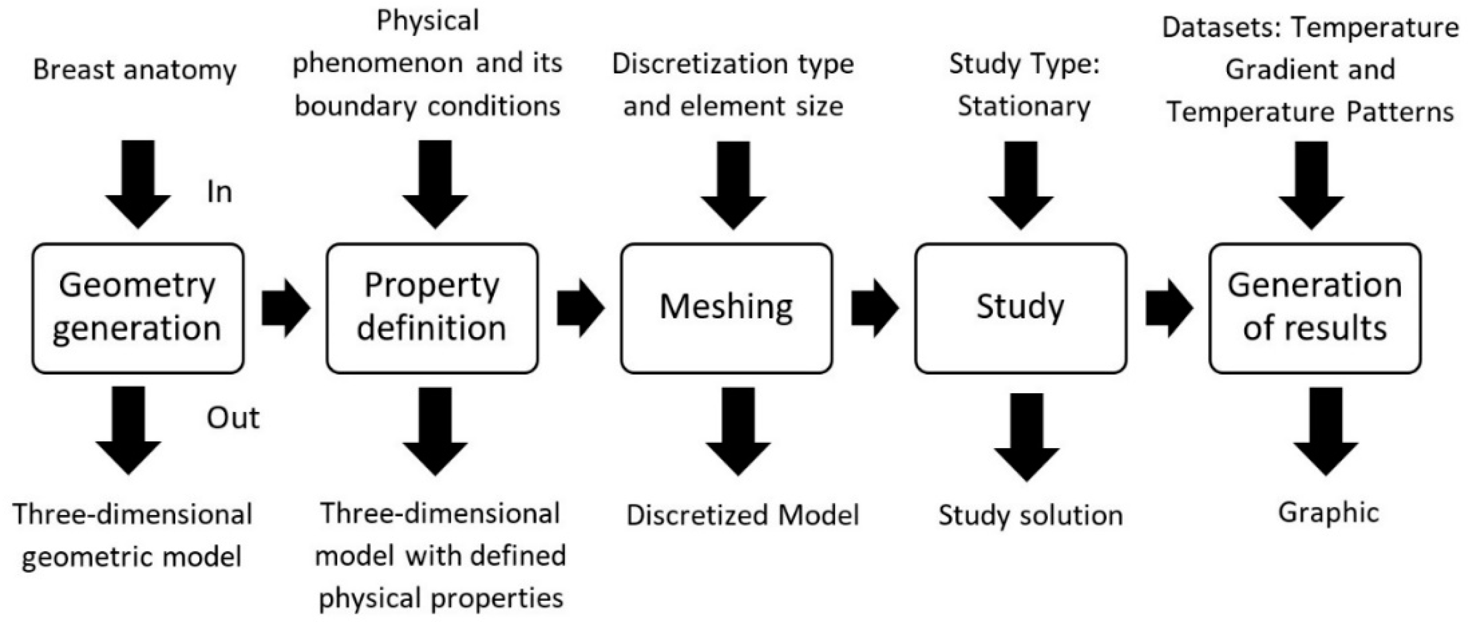
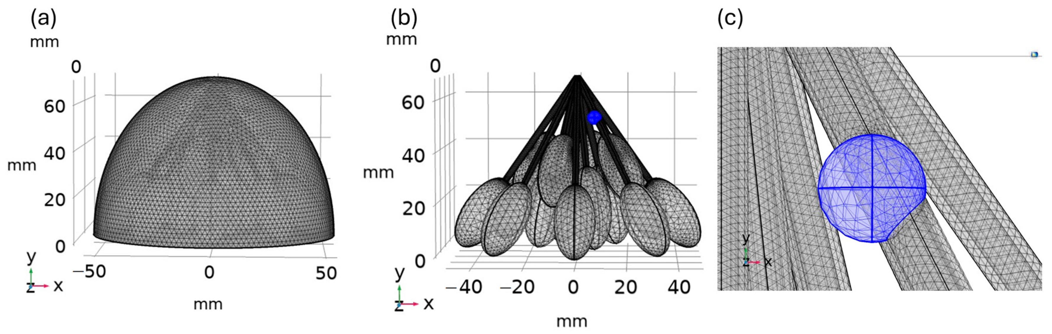
2.2. Finite Element Method and the Computational Modelling

The objective of the finite element method is to obtain information about the system from its geometric model, working by means of the subdivision of the domain into smaller and simpler elements. These elements are defined by nodes, where each one is associated with a set of shape functions that allow us to interpolate data between nodes. According to the model’s dimensions (1D, 2D or 3D), each shape function is defined with certain degrees of freedom. Subsequently, the Galerkin approach can be used, and the solution field is constructed from the solution vector and the set of the basic shape functions in all elements [45].

The geometric model considered in this work consists of a three-dimensional structure defined by the skin, fat, gland, and tumor domains. It was based on the breast model reported in Acero [46]. In that work, the model was validated by means of a comparative analysis with the results obtained by [17], obtaining satisfactory results. The breast was modeled as a hemisphere with a diameter of 11.0 cm and height of 7.2 cm; it contains a glandular tissue composed of 16 lobes, with each one connected (Figure 2b) to a galactophore conduct. The domains corresponding to the epidermis and dermis layers were merged to simulate the skin (Figure 2a). This model allowed to obtain internal thermal gradients close to those of a real situation, as was demonstrated in [46], due to the geometry being nearly attached to the anatomy of the mammary gland. This is unlike other works which use layers to represent different domains, making it impossible to obtain gradients related to a tumor’s location and size inside the breast. Another fact is that all parameter values used in the simulation were obtained from previous works, where the used data were taken from real cases or estimated from the computation of data extracted from real tissues.

The geometric design of the model was produced in SolidWorks^® and imported by COMSOL Multiphysics^® in order to simulate the thermal phenomenon. The mesh of the model is depicted in Figure 2. The model was solved for different cases, such as for three tumor sizes (5 mm, 6 mm, and 8 mm) and a case without a tumor (healthy). The features of each simulated model were the number of elements—1540413, 1537284, 1541649, and 1521349; degrees of freedom—2072848 (internal: 759749), 2068621 (internal: 758977), 2074458 (internal: 760733), and 2047357 (internal: 747933); physical memory—7.7 GB, 6.46 GB, 6.49 GB, and 6.44 GB; virtual memory—11.38 GB, 8.98 GB, 9.23 GB, and 9.18 GB; and number of nodes—2072848 (internal: 759749), 2068621 (internal: 758977), 2074458 (internal: 760733), and 2047357 (internal: 747933). This was performed for tumor sizes of 5 mm, 6 mm, and 8 mm and for healthy tumors, respectively.

2.3. Simulation Properties

The simulation focuses on tumors with a diameter of 5, 6, and 8 mm and all tumors located at a depth of 15 mm from the skin surface, specifically inside of one of the milk ducts. A healthy case (without a tumor) was considered too. It was used as a reference for when a temperature increase associated with a lesion was not present.

The tissue properties defined in the computational model were thermal capacity (C_p), thermal conductivity (K), density (ρ), and heat generation rate (Q_m).

These properties were defined based on data reported in previous works and that had been validated to be typical values accepted in the breast modelling field. The considered values and the references they were taken from are shown in

Table 1. Thermophysical properties of tissues.

Domain	Property
	Cp [J/(kg °C)]	K [W/(m °C)]	ρ [kg/m3]	Qm [W/m3]
Fat	2348 [48]	0.21 [11,48]	911 [48]	400 [19]
Gland	3475 [10]	0.48 [19]	1080 [19]	700 [19]
Tumor	3475 [10]	0.48 [19]	1080 [19]	VAR [20]
Dermis	3475 [10]	0.3140 [10]	1050 [10]	368.1 [17]
Epidermis	3475 [10]	0.2093 [10]	1050 [10]	0 [17]

VAR means variable. Value depends on tumor case.

. In the case of the heat generation rate of tumors, the fundamental equation proposed by Gautherie [47] to calculate Q_m from tumor diameters was not applied due to it just being valid for tumors with a diameter ≥ 10 mm. Then, values approximated from real cases by [20] using a dynamic neural network were considered.

In addition to previously mentioned parameters, among the thermophysical properties considered were those corresponding to blood for each domain; these were obtained from Ng and Sudharsan [19] and Chanmugam [17]. They are shown in

Table 2. Thermophysical properties of blood.

Domain	Property
	Ta [°C]	Cp,b [J/(kg °C)]	Wb [1/s]	ρb [kg/m3]
Fat	37	4200	0.0002	1060
Gland	37	4200	0.0006	1060
Tumor	37	4200	0.012	1060
Dermis	37	4200	0.0002	1200
Epidermis	37	4200	0	1200

.

For all domains, the initial temperature value was set to 37 °C. As boundary conditions, a fixed temperature was assigned for the thoracic wall equal to an arterial temperature of 37 °C and convective heat flux was added to the upper contour of the dome (counterpart to the epidermis), with a coefficient of heat transfer of 13.5 [W/(m² °C)] and with an environmental temperature of 20 °C.

Regarding the mesh, a tetrahedral element of the second order was used; the maximum and minimum element sizes were 3.9 mm and 0.167 mm, respectively, as shown in Figure 1. For the simulated models, the discretization time was 1 min 3 s, 1 min 5 s, 1 min 7 s, and 1 min 10 s and the simulation time was 1 min 49 s, 1 min 49 s, 1 min 51 s, and 2 min 55 s for tumor sizes of 5 mm, 6 mm, and 8 mm, and for healthy tissue, respectively.

2.4. Case Study: Stationary for 5, 6, and 8 mm Tumors and Healthy Tissue

The study was simulated in a steady state. The values of Q_m for tumors were taken as 120,800 W/m³, 60,830 W/m³ and 68,450 W/m³ for diameters of 5, 6, and 8 mm, respectively. A model of a breast including a tumor is shown in Figure 3. Straight lines were inserted to show how the vertical (Figure 3a) and horizontal (Figure 3b) paths along the gradients were estimated. Both paths were marked with points to indicate the coordinates of the interfaces between the involved tissues. Each path was positioned such that it crossed the tumor’s center.

The vertical path extends from the chest wall to the surface of the breast. Point P₃ corresponds to the posterior fat–tumor interface, and its y coordinate value depends on the tumor size due to the anterior face of all tumors being positioned at 15 mm of depth. The y coordinates corresponding to point P₃ were specified in decreasing order of tumor size.

The horizontal path extends from one side (P₀) to the opposite side (P_f) of the breast. The coordinates for each tumor size are summarized in

Table 3. The X coordinates of the points of interest for tumors with a diameter of 5, 6, and 8 mm (Horizontal path).

Tumor Size (Diameter [mm])	P0 [mm]	P1 [mm]	P2 [mm]	P3 [mm]	P4 [mm]	P5 [mm]	P6 [mm]	P7 [mm]	P8 [mm]	Pf [mm]
5	−36.23	−34.10	−9.34	−6.76	−4.2	−2.14	4.5	9.5	34.1	36.23
6	−36.66	−34.54	−9.62	−6.88	−4.56	−2.14	4	10	34.54	36.66
8	−37.47	−35.40	−10.05	−7.25	−4.76	−2.06	3	11	35.40	37.48

. They were different in each case due to the position of the tumor center varying with tumor size.

Once the study was completed, superficial and internal thermal distributions were obtained. Their respective gradients were estimated from the derivative of thermal distribution data

$$\left|{\nabla }_{x}T\right|=\frac{\delta T}{\delta x}=\frac{T\left(x_{n+1},y_n\right)-T(x_n,y_n)}{x_{n+1}-x_n}$$

(2)

$$\left|{\nabla }_{y}T\right|=\frac{\delta T}{\delta y}=\frac{T\left(x_n,y_{n+1}\right)-T(x_n,y_n)}{y_{n+1}-y_n}$$

(3)

$$\left|{\nabla }_{L}T\right|=\frac{\delta T}{\delta L}=\frac{T\left(L_{n+1}\right)-T\left(L_n\right)}{L_{n+1}-L_n}$$

(4)

Internal gradients were obtained along the vertical (x) and the horizontal (y) axes defined in the model. In the case of the superficial gradient, it was calculated along the arc length (L) of an arc path, defined in relation to the simulated breast surface.

3. Results

In this section, the results obtained from model simulation are presented. As a first section, quantitative analysis of internal temperature distributions and their respective temperature gradients are described for three cases with different tumor sizes, taking the healthy case as a reference. The behavior of internal temperature and its gradients along the horizontal and vertical paths are analyzed. In the second section, temperature distributions over the breast model surface are presented for the three cases too. In order to quantify the main indicators detected in the models, superficial temperatures are graphed and examined over an arc path traced above the tumor locations.

3.1. Results from Internal Analysis for Breast with Tumors and Healthy Tissue

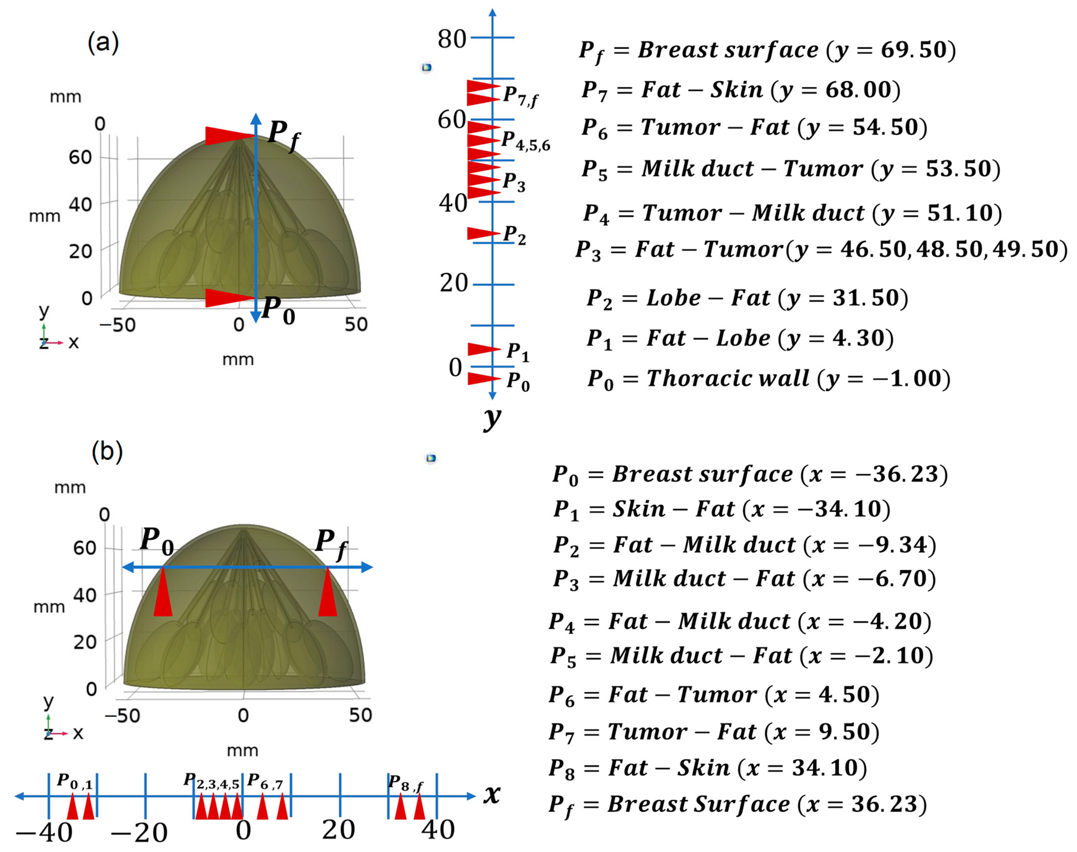
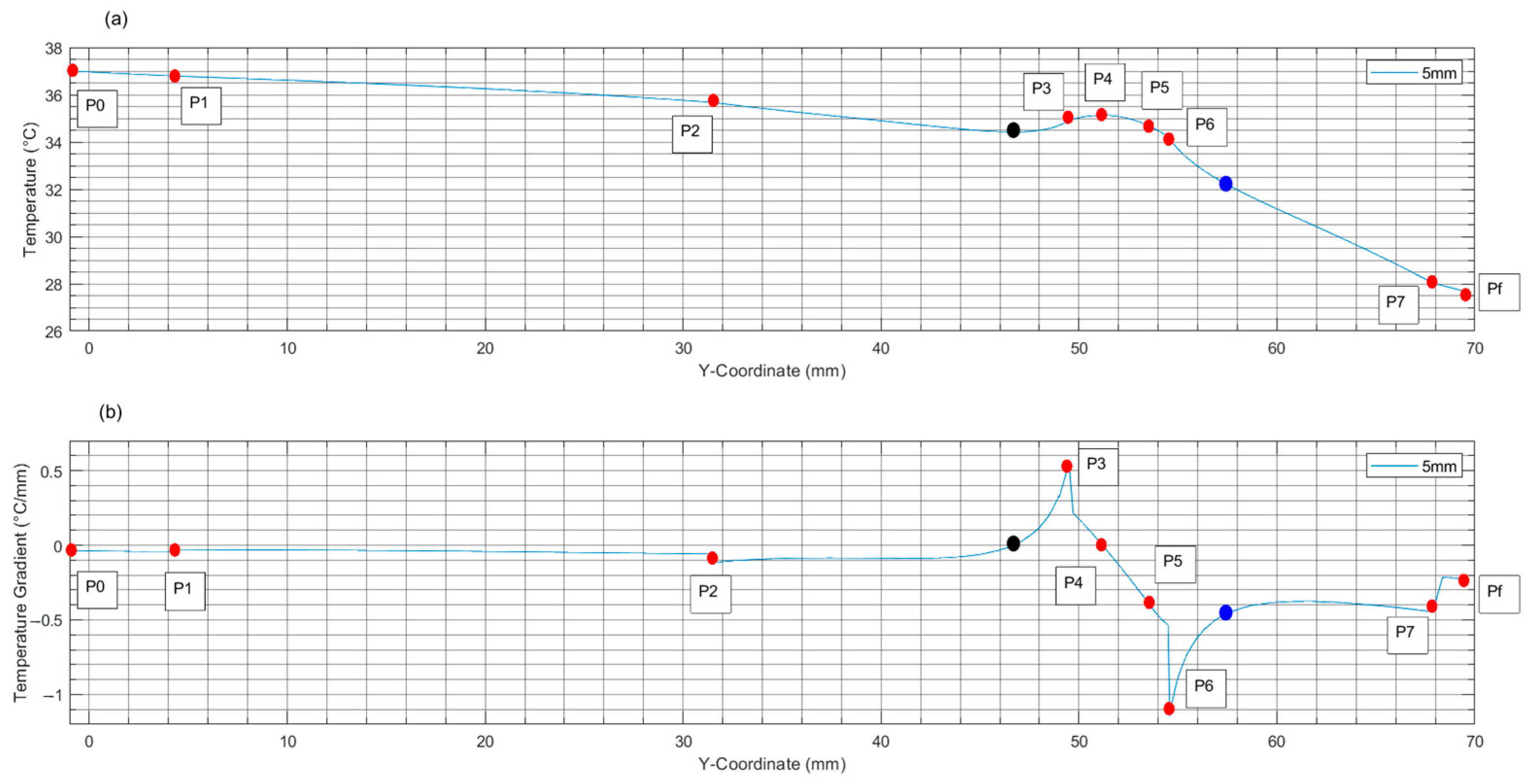
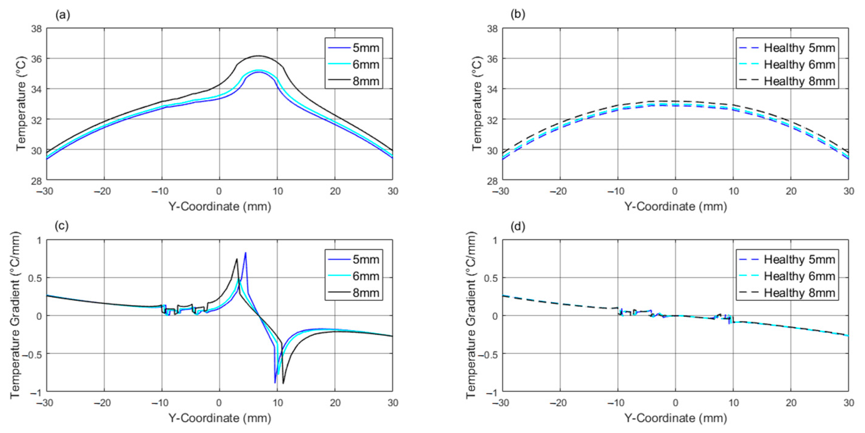
3.1.1. Vertical Internal Path

To illustrate temperature and gradient behaviors, the case of a breast model containing a tumor with a diameter of 5 mm was selected. In Figure 4, the temperature distribution and its corresponding gradient are plotted along a vertical path crossing the tumor. Analyzing the temperature distribution and the gradient it produced from the chest wall to the breast surface, it was noticed that a temperature of 37 °C was established at the thoracic region (P₀). This slowly decreased (at an average rate of −0.06 °C/mm) to a minimum value of 34.42 °C at a point (black point) located 2.78 mm before P₃, which corresponded to the fat–tumor interface (Figure 4a). In the temperature gradient graph (Figure 4b), as expected, this black point corresponded to a zero crossing. This point was defined as the beginning of the zone warmed by tumor growth (ZWTG). From this point until P₃, the temperature rose at an average rate of 0.19 °C/mm, producing an abnormal thermal distribution in the healthy zone surrounding the tumor.

The maximum rate was reached at P₃, which corresponded to the tumor boundary, and was equal to 0.55 °C/mm. After P₃ and until P₄, the temperature continued increasing, but the average rate presented a slight decrease; it was equal to 0.13 °C/mm. The warmest point in the tumoral zone was in P_4, with a temperature of 35.13 °C. From this point, the temperature decreased at an average rate equal to −0.17 °C/mm until P₅, a point that corresponded to the interface between a galactophore duct and the tumor. Near to the tumor–fat boundary, P₆, there was a zone inside the tumor (with a depth of 1.03 mm measured from the boundary) with the largest average decreasing rate (−0.52 °C/mm), reaching a maximum value of −1.14 °C/mm at exactly the boundary. Following the path into the healthy fatty tissue, the average decreasing rate in the next 2.78 mm (assessed to consider a symmetrical heating profile before and after tumor formation) was equal to −0.77 °C/mm. The end point of the 2.78 mm segment is marked with a blue point in the figure. Thus, the ZWTG is considered to be the zone between black and blue points. The final segment, from the blue point to the breast surface (P_f), was composed of fat and skin tissues, where temperature continued decreasing at an average rate equal to −0.38 °C/mm. The temperature on the breast surface was 27.67 °C.

In

Table 4. Temperature and gradient values for marked points in the vertical path. Cases of breast with tumors of 5 mm, 6 mm, and 8 mm in diameter and healthy case are included.

T. D. [mm]		Healthy Tissue				Tumoral Zone				Healthy Tissue
					Zone Warmed by Tumor Growth (ZWTG)
		P0	P1	P2	(a) Black Point	P3	P4	P5	P6	(b) Blue Point	P7	Pf
5	T $\nabla$T	37 −0.037	36.79 −0.029	35.68 −0.058	34.42 ≈0	34.92 0.547	35.13 ≈0	34.67 −0.399	34.12 −1.144	32.21 −0.459	28.03 −0.446	27.67 −0.224
6	T $\nabla$T	37.00 −0.029	36.79 −0.029	35.69 −0.057	34.64 ≈0	34.96 0.340	35.24 −0.085	34.69 −0.384	34.16 −1.035	32.26 −0.464	28.06 −0.448	27.69 −0.225
8	T $\nabla$T	37.00 −0.036	36.79 −0.028	35.76 −0.049	35.19 ≈0	35.73 0.375	36.06 −0.157	35.39 −0.413	34.84 −1.089	31.90 −0.457	28.17 −0.459	27.80 −0.229
Healthy	T $\nabla$T	37.00 −0.038	36.79 −0.029	35.63 −0.064	--	--	32.88 −0.174	32.45 −0.216	--	-- --	27.88 −0.431	27.53 −0.219

^(a) Black point was located 2.78 mm, 3.03 mm and 4.53 mm before P₃ for each tumor 5 mm, 6 mm, and 8 mm, respectively. ^(b) Blue point was located 2.78 mm, 3.03 mm, and 4.53 mm after P₆ for each tumor 5 mm, 6 mm, and 8 mm, respectively. T. D.: tumor diameter. T indicates temperature (°C) and $\nabla$T indicates gradient (°C/mm) in the corresponding point. The shadowed zone corresponds to information about points inside the tumor and the columns (points) highlighted by a red line correspond to points in the zone warmed by tumors.

, the relevant values of temperature and gradients for all tumor sizes along vertical path are summarized. In all cases, the maximum positive and negative gradient values were identified at the posterior (P₃) and anterior (P₆) boundaries of the tumor, respectively. Temperature distributions along vertical paths for all cases, with tumor and healthy, and their respective gradients are displayed in Figure 5.

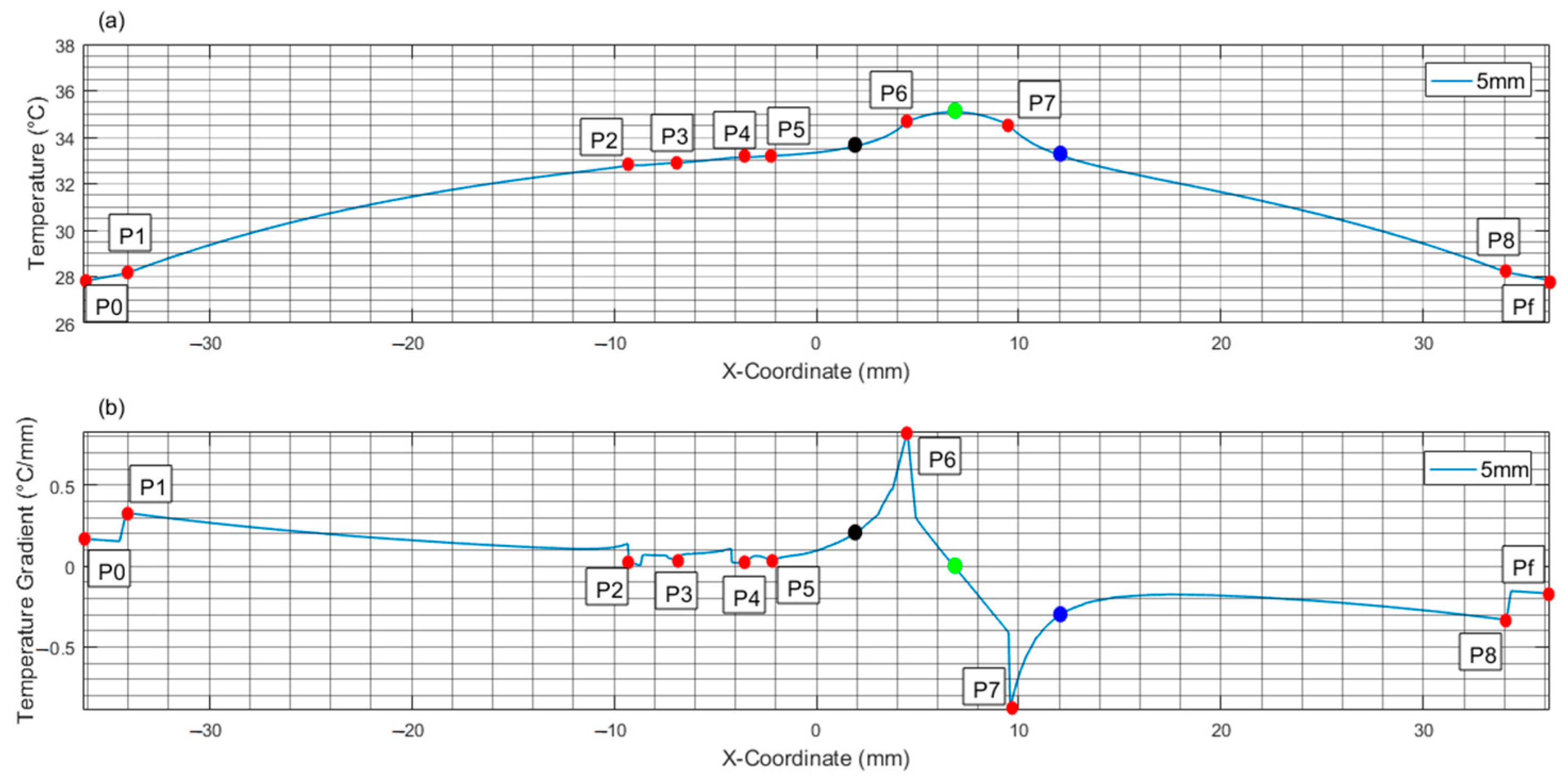
3.1.2. Horizontal Internal Path

In the case of a horizontal path, Figure 6 shows the temperature distribution and its corresponding gradient for the same case as that detailed for the vertical path, a case of a tumor with a diameter of 5 mm. A horizontal path was drawn from one end to the other of the breast surface, and we ensured that it crossed the tumor center (Figure 3). At the initial point, P₀, located on the left side of the breast surface, the temperature was equal to 27.8 °C, increasing with depth over the path at an average rate of 0.11 °C/mm until the point corresponding to a coordinate x = 0 mm. At this point, the temperature was equal to 33.33 °C; this trajectory was followed over the healthy half of the breast. From this point (even a bit before) until the black point, a slight rise in the average rate was noticed due to the presence of tumor, reaching a value equal to 0.14 °C/mm. Nevertheless, between the black point and P₆ (which is the left boundary of tumor), the average rate tripled; it was equal to 0.41 °C/mm. In terms of gradient (punctual rate), the black point had a value equal to 24% of the maximum gradient, which was reached at point P₆. And in terms of temperature, this point compared to the same point in the healthy case presented a temperature increment of 2.3%. The distance between the black point and P₆ was equal to 2.52 mm. This was a value close to the 2.78 mm found on the vertical path and was defined as the length of a healthy surrounding ZWTG. For this reason, in the case of the horizontal path, the black point was also considered as the beginning of the healthy ZWTG. And taking the same distance (2.52 mm) from the right boundary of tumor, P₇, a blue point was marked to delimitate the warmed healthy zone in this orientation too.

The area from point P₆ to point P₇ corresponds to the tumoral zone. The highest temperature in this region is 35.0 °C. This occurs at a coordinate x = 6.79 mm, almost at the tumor center. This point is marked with a green point, which corresponds, as expected, to a zero crossing in the temperature gradient graph.

Points P₆ and P₇, corresponding to the left and the right boundaries of the tumor, coincided with the maximum positive (0.83 °C/mm) and the maximum negative (−0.89 °C/mm) values of the temperature gradient, respectively, and did so in the vertical case. The average increasing rate between P₆ and the green point was 0.16 °C/mm, and the average decreasing rate between green point and P₇ was −0.22 °C/mm.

The average decrease rate between P₇ and the blue point was −0.56 °C/mm; after this point, the average decrease rate diminished to a value of −0.23 °C/mm until the other side of the breast surface, which presented a temperature of 27.8 °C.

In

Table 5. Temperature and gradient values for marked points in the horizontal path. Cases of breasts with tumors of 5 mm, 6 mm and 8 mm in diameter and a healthy case are included.

T. D. [mm]		Healthy Tissue							Tumoral Zone			Healthy Tissue
								Zone Warmed by Tumor Growth (ZWTG)
		P0	P1	P2	P3	P4	P5	(a) Black Point	P6	(b) Green Point	P7	(c) Blue Point	P8	Pf
5	T $\nabla$T	27.79 0.167	28.13 0.328	32.79 0.016	32.9 0.030	33.13 0.025	33.20 0.034	33.62 0.199	34.67 0.831	35.08 ≈ 0	34.53 −0.890	33.22 −0.301	28.18 −0.333	27.84 −0.170
H. E. C.	T $\nabla$T	27.79 0.167	28.13 0.328	32.67 0.016	32.75 0.016	32.88 ≈0	32.9 −0.028	-- --	32.8 −0.030	32.73 −0.011	32.65 −0.103	-- --	28.15 −0.330	27.8 −0.167
6	T $\nabla$T	27.81 0.169	28.15 0.332	32.89 0.028	33.02 0.029	33.27 0.014	33.36 0.044	33.55 0.118	34.79 0.490	35.21 ≈ 0	34.63 −0.775	33.00 −0.239	28.20 −0.337	27.85 −0.172
H. E. C.	T $\nabla$T	27.80 0.169	28.14 0.331	32.75 0.016	32.84 0.011	32.97 −0.023	32.99 ≈0	-- --	32.92 −0.021	32.83 −0.039	32.71 −0.092	-- --	28.16 −0.333	27.82 −0.170
8	T $\nabla$T	27.84 0.173	28.18 0.340	33.16 0.044	33.33 0.034	33.67 0.023	33.86 0.070	34.04 0.180	35.56 0.749	36.15 ≈ 0	35.38 −0.898	33.4 −0.288	28.25 −0.347	27.90 −0.177
H. E. C.	T $\nabla$T	27.82 0.172	28.16 0.338	32.92 0.025	33.01 ≈0	33.15 −0.015	33.17 0.011	-- --	33.14 −0.019	33.03 −0.046	32.84 −0.082	-- --	28.18 −0.340	27.84 −0.172

^(a) Black point was located 2.52 mm, 3.38 mm and 4.10 mm before P₆ for 5 mm, 6 mm, and 8 mm tumors, respectively. ^(b) Green point was located in the position x = 6.79 mm, x = 6.79 mm, and x = 6.69 mm for 5 mm, 6 mm, and 8 mm tumors, respectively. ^(c) Blue point was located 2.52 mm, 3.38 mm, and 4.10 mm after P₇ for 5 mm, 6 mm, and 8 mm tumors, respectively. T. D.: tumor diameter. H. E. C.: healthy equivalent case. T indicates temperature (°C) and $\nabla$T indicates gradient (°C/mm) in the corresponding point. The shadowed zone corresponds to information of points inside the tumor and the columns (points) highlighted by the red line correspond to points in the zone that is warmed by tumors.

, the relevant values, analyzed previously for the breast with a tumor of 5 mm, are listed for all cases considering the horizontal path. In all tumor sizes, the black point is placed in the position corresponding to 24% of the maximum gradient value, which in all cases is reached at P₆. Regarding temperature, the black point corresponds to increments of 1.75% and 2.62% compared to the equivalent points in the corresponding healthy cases for tumors of 6 and 8 mm, respectively.

Figure 7 shows temperature distributions along horizontal path and their respective gradients for all models, both cases with tumors and their respective healthy cases.

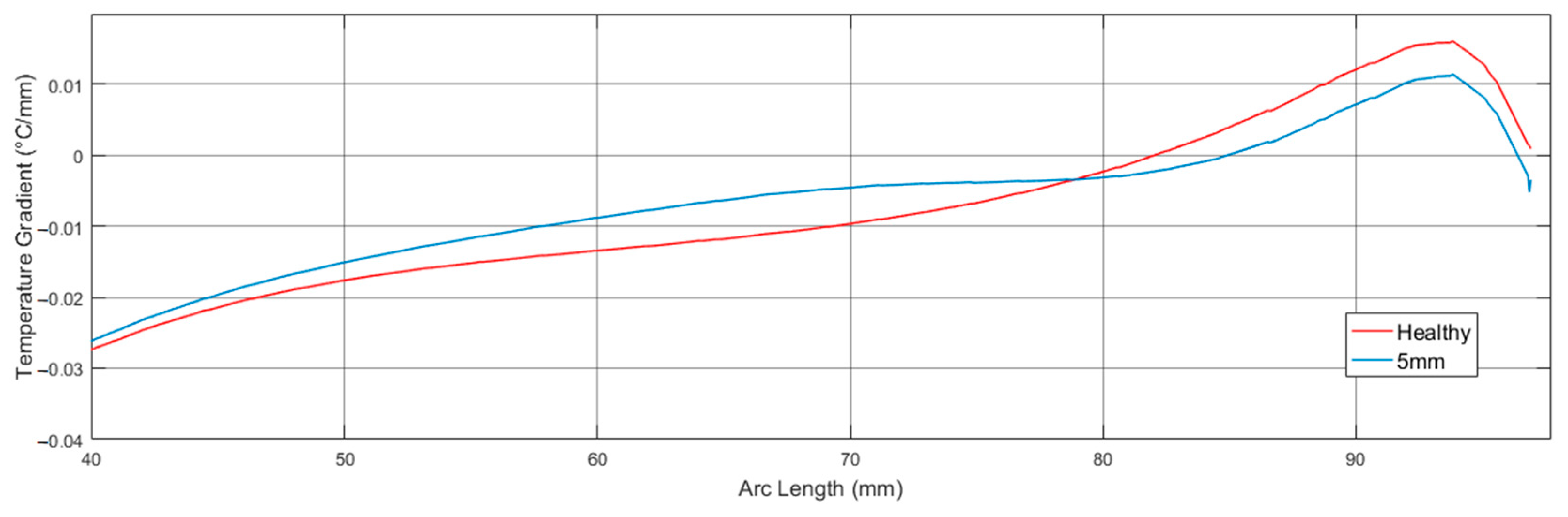
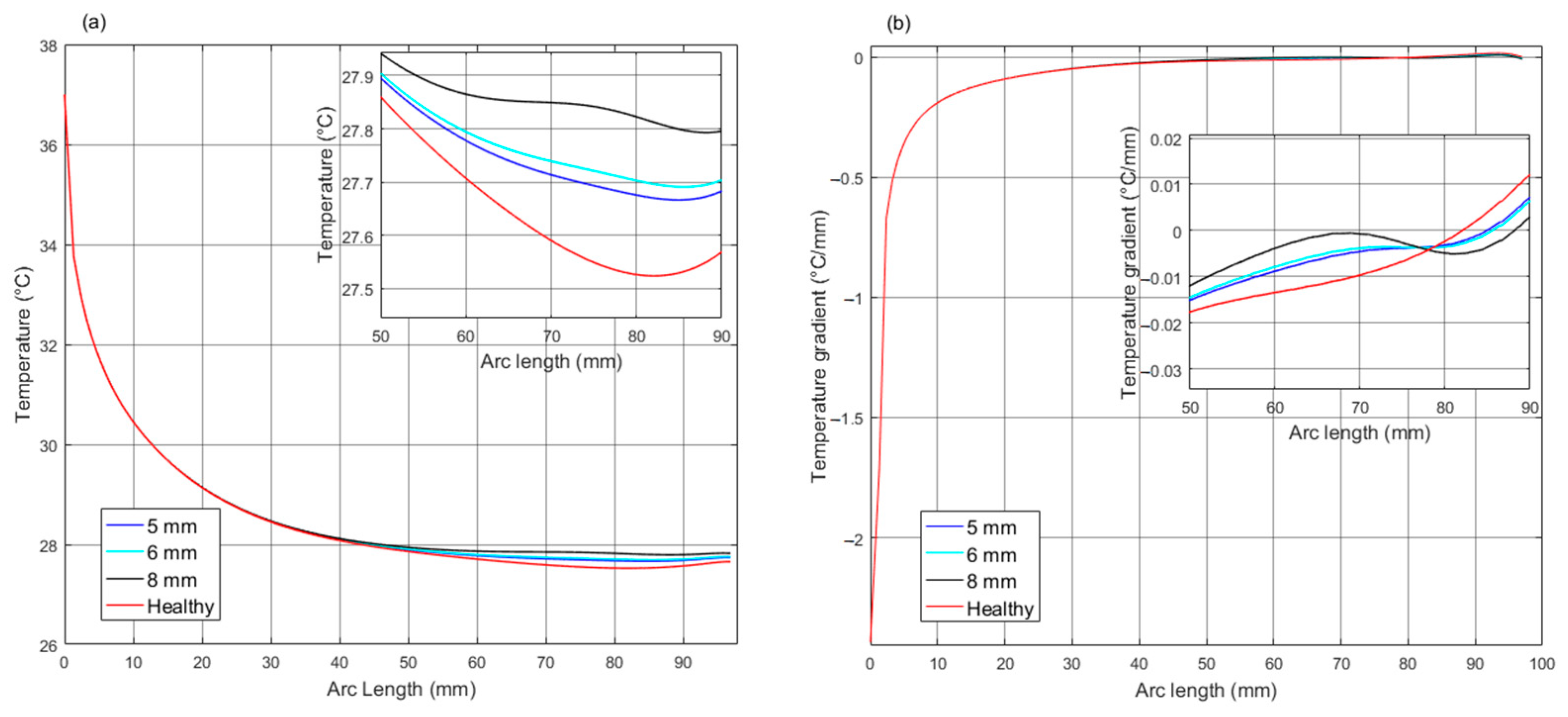
3.2. Results from Superficial Temperatures for Breast with Tumors and Healthy Tissue

In this section, a quantitative analysis of thermal data from the breast surface is presented. As a reference, in Figure 8, thermal distribution maps for the cases of healthy breast (Figure 8a), breast with a tumor of 5 mm in diameter (Figure 8b), 6 mm (Figure 8c), and 8 mm (Figure 8d) are shown. It is appreciated that, for the breast with the smallest tumor (5 mm), the temperature variations on the surface section above the tumor’s location showed values of less than 0.1 °C. All tumor centers were approximately located at the coordinates x = 7.0 mm; y = 52, 51.5, and 50.5 mm (for tumors of 5, 6, and 8 mm in diameter, respectively); and z = 7.5 mm. All of them were located at 15 mm of depth from the surface, measured along the y axis.

In all cases, the highest temperature (37 °C) was found in the base of the breast (stuck to the chest). In the healthy case, it decreased uniformly as breast surface (“skin”) approached the nipple, where a slight increment was detected. In tumoral cases, an abnormal temperature rise, proportional to tumor size, was produced in the quadrant of tumor location. These increments influenced the nipple zone proportionally to the tumor size too.

To analyze data numerically, as performed in the internal analysis, temperatures along the arc path, indicated with a dotted line in Figure 8, were extracted from all models. As an example, temperatures over this path for the case of tumors of 5 mm are displayed in Figure 9 with a blue line. Remarking on temperature elevation due to the tumor’s presence, the temperatures over the same arc path for the healthy case were included in the graph with a red line. The arc length (L) points equal to 0 mm corresponded to the base of the breast, meaning it was stuck to the thoracic wall, and the arc length point of 97 mm corresponded to the nipple center. Surface temperatures along the arc of both cases were compared. We remark on two aspects: (i) the temperature difference remained under 0.1 °C until 65.67 mm; (ii) it grew slowly until reaching a maximum value of 0.15 °C at 78.88 mm, which is marked with a dotted line in the zoomed-in image included in the graph.

The temperature gradient over the arc length was computed for both cases described above (Figure 10). As expected, negative (or decreasing) gradient values prevailed along the arc length, being larger (in magnitude) for the healthy model. This meant that the temperature decayed faster in it until 78.88 mm, where the gradients began to be greater than in the case of tumors. The minimum temperatures (zero-crossing gradient) were reached at 82.02 mm and at 84.92 mm for the breast without and with tumors, respectively. Regarding positive gradient values, they were smaller for the latter, which implies that a tumor attenuates the natural gradient values present at the end of the arc path (near to the nipple).

In

Table 6. Parameters related to temperature and gradient behavior estimated on the arc length traced on breast surface.

Tumor Diameter	(A) Maximum Temperature Difference with Respect to Healthy Case	(B) Arc Length of Maximum Temperature Difference	(C) Arc Length of Zero Crossing in the Gradient Graph	(D) Arc Length of Intersection with Gradient of Healthy Case
(mm)	(°C)	(mm)	(mm)	(mm)
5	0.15	78.88	84.92	78.88
6	0.18	78.64	85.55	78.64
8	0.30	78.03	88.15	78.03
Healthy	--	--	82.02	--

, parameters related to surface temperature and the associated gradient for all tumor sizes are listed.

Temperature distributions and their corresponding gradients over the arc lengths are graphed in Figure 11 for all cases. The proportionality between tumor size and temperature distribution was noticeable. In this case, the gradient magnitudes were also directly proportional to tumor size.

In the following section, there is a discussion about how the parameters estimated with the thermal simulations and the obtained gradients could be associated with important indicators related to tumor stage and malignancy.

4. Discussion

There are several tumor parameters to be predicted based on thermal information acquired from tumoral zones: depth, size, shape, malignancy grade, internal composition, metastasis stage, etc. However, first- or second-level sanitary attention would be desirable to know the most relevant malignancy probability and size, and if metastasis is present, although the last one can be deduced from the first two most of the times. In the analysis presented here, we tried to relate the temperature and gradient data, extracted from simulations that were nearly attached to real situations, to tumor characteristics. On the one hand, it was shown that internal and external temperature distributions are influenced by tumor size. In Figure 5a, Figure 7a, and Figure 11a, the temperature behaviors along different paths (internal/vertical, internal/horizontal, and external arc, respectively) involving tumoral zone are presented and in all of them a direct relation between temperature increase and tumor size is observed: the smaller the tumor, the lesser the temperature increase. A Kruskal–Willis test was carried out to analyze the differences between the thermal distributions and healthy case. It was observed that a greater increase in temperature was presented with a tumor size of 8 mm with respect to tumor sizes of 5 mm and 6 mm (p < 0.05). Nevertheless, between the tumors of 5 mm and 6 mm, a significant difference was not observed. It was even possible, based on data from the internal paths, to define the ZWTG, which is related with tumor size too: we proposed to mark the first zero-crossing point of the vertical gradient (called black point) as the beginning of this zone. This was mainly carried out due to this point representing the first change in the gradient’s direction from a negative to positive one, which means a thermal tendency switch from tissue cooling (healthy tissue) to tissue heating (tumor). The distance between the black point and tumor boundary was measured based on the vertical gradient; it was defined as the difference between the location of the black point and location of the maximum positive peak of the gradient that corresponded to the tumor beginning. To keep symmetry in the ZWTG, this distance was measured from the tumor end’s to the healthy tissue after the tumor to mark the so-called blue point, which represents the end of the ZWTG. In Table 4, the distances between tumor boundaries and black and blue points are described for each tumor size in the footnotes. These distances added to tumor size results in the ZWTG length over the vertical path.

Table 7. ZWTG lengths over vertical paths for tumors of 5, 6, and 8 mm in diameter.

Tumor Diam. (mm)	Distances from Blue and Black Points to Tumor Boundaries (mm)	ZWTG (mm)
TS	Dv	Lv = TS + 2Dv
5	2.78	10.56
6	3.03	12.06
8	4.53	17.06

shows the ZWTG lengths measured on the vertical path for each tumor size based on the information extracted from the gradient. In all cases, ZWTG’s vertical length doubles the tumor’s diameter.

For the horizontal path, a similar procedure was defined, and results close to those of the vertical case were obtained. In

Table 8. ZWTG lengths over horizontal path for tumors of 5, 6, and 8 mm in diameter.

Tumor Diam. (mm)	Distances from Blue and Black Points to Tumor Boundaries (mm)	ZWTG (mm)
TS	Dh	Lh = TS + 2Dh
5	2.52	10.04
6	3.38	12.76
8	4.10	16.20

, the ZWTG horizontal lengths are listed for each tumor size; in this case, it also doubles the tumor diameter. It can be appreciated that our defined warmed zone (ZWTG) did not reach the surface in any case; however, in the superficial temperature distribution, as we will analyze later on, there were tiny temperature increments that depended on tumor size.

It is important to note that, following our analysis based on the data of internal temperature distribution, it was possible to obtain the size of a hypothetical real tumor from the maximum and minimum values of the computed gradient and to determine the corresponding ZWTG vertical length from the zero-crossing point of the same gradient.

Another important parameter associated with gradient characteristics is the heat generation rate (Q_m), which is directly related to tumor malignancy [37,38]. The maximum peaks of the gradient graphs always correspond to tumor boundaries, meaning to tumor interfaces with healthy tissues which present very low Q_m values compared with tumors, creating abrupt changes that are perceptible in the gradient graph as these maximum peaks. The magnitude of the gradient peaks (positive or negative) was proportional to the tumor Q_m independently of tumor size; the higher the Q_m, the higher the gradient magnitude. This relation is shown in Figure 5b and in Figure 7c, where the vertical and horizontal gradients are graphed for all tumor sizes; however, to provide an overall view, the magnitudes of gradient peaks corresponding to tumor boundaries are listed in

Table 9. Magnitude of gradient peaks related to tumor boundaries.

Tumor Diam. (mm)	Qm W/m3	Gradient Peak Magnitude (°C/mm)
		Vertical Path		Horizontal Path
		Posterior Boundary (P3V)	Anterior Boundary (P6V)	Right Boundary (P6H)	Left Boundary (P7H)
5	120,800	0.547	1.144	0.831	0.890
6	60,830	0.340	1.035	0.490	0.775
8	68,450	0.375	1.089	0.749	0.898

for the three tumor cases. The largest value of Q_m belongs to the smallest tumor (D = 5 mm). It presents the greatest magnitudes of gradient peaks, following the tumor with a diameter of 8 mm, which has a Q_m equal to 68,450 W/m³, and lastly the tumor with a diameter of 6 mm, whose Q_m is equal to 60,830 W/m³ and which presents the smallest peak values. All boundaries listed in the table were composed of tumoral and fatty tissues, due to simulated tumors developing as ductal neoplasia surrounded by fat. The boundaries situated nearest to the breast surface, meaning the anterior and left ones, had gradient peak magnitudes greater than the other two boundaries, which are located deeper from the surface. It could be due to the temperature distribution towards the surface changing more drastically than that at the other sides. In this case, the Kruskal–Willis test was applied, considering the differences between the tumor gradients and the healthy one. The results indicate that, in the vertical and horizontal paths, the tumor of 5 mm was distinguishable from the others (p < 0.05). No significant difference was observed between tumors of 6 mm and 8 mm.

In cases of superficial temperature distributions, both temperature increments and gradients behaved in accordance with tumor size: the larger the tumor size, the higher temperature increase, and the higher gradient “peak” magnitude. However, in superficial gradients, these peaks were smoothed compared with those present at the internal distributions.

The size of the warmed superficial area also correlated with tumor size. However, from the smallest tumor, the warmed area covered the entire lower right quadrant, complicating efforts to locate the exact position of tumors.

To evaluate the accuracy that could be reached in a supposed case where just external temperature and gradient information were available, an analysis of the projection, over the x axis, of the points of maximum temperatures and maximum gradient differences regarding healthy cases was performed. In

Table 10. Projection of magnitude of gradient peaks related to tumor (mm).

A.	B1.	B2.	B3.	C.	D.	E.	F.	G.	H.
Tumor Diam	Location of Tumor Projected on x Axis			Arc Length of Maximum Temp Diff	Projection of (C) on x Axis	Dist. from (D) to Center	Arc Length of Maximum Grad Diff	Projection of (F) on x Axis	Dist. from (G) to Center
	Left Bound (P6H)	Right Bound (P7H)	Center
5	4.50	9.5	7.00	78.88	3.15	3.85	67.62	6.40	0.60
6	4.00	10.00	7.00	78.64	3.25	3.75	66.51	6.80	0.20
8	3.00	11.00	7.00	78.03	3.35	3.65	64.67	7.50	−0.50

, the first four columns show the tumor size (A), the projection of its left bound’s location on the x axis (B1), that of its right bound, (B2), and that of its center (B3). The arc lengths and their projections on the x axis corresponding to the location of maximum temperature difference regarding with healthy case were listed in columns C and D for the three cases. Next, the distance of this projected point (D) to the projection of the tumor’s center (B3) was registered in column E. It diminished as the tumor’s diameter increased; the reason for this was that the projection of the maximum temperature difference moved to the left.

The same steps were followed for the case of maximum gradient difference regarding a healthy gradient. The arc length corresponding to the position of this point and its projection on x axis are listed in columns F and G, respectively. The distance from the projected point (G) to the tumor center (B3) was presented in column H. In this case, the obtained distances to tumor centers were smaller than those obtained when considering temperature differences. Distances from the points of maximum gradient differences to tumor centers were in the order of a tenth of a millimeter (column H). Thus, a preliminary observation is that when trying to locate, as accurately as possible, a tumor’s location based on external temperature distribution data, according to our analysis, it is better to take as reference the point of maximum difference between gradients than the point of maximum difference between temperatures. The mean and standard deviations of the values considered in columns E (maximum temperature projection) and H (maximum gradient projection) were 3.75 (±0.10) and 0.43 (±0.21), respectively.

Finally, maximum temperature increments with regard to healthy cases were computed for all tumor cases in the three paths: vertical, horizontal, and superficial. In

Table 11. Maximum temperature increments for all tumoral cases.

Tumor Diam. (mm)	Path
	Vertical		Horizontal		Superficial
	Temp Diff (°C)	Y Coord (mm)	Temp Diff (°C)	X Coord (mm)	Temp Diff (°C)	Arc Length (mm)
5	2.36	52.34	2.35	6.86	0.15	78.88
6	2.40	52.06	2.39	6.89	0.18	78.64
8	3.17	51.35	3.14	7.2	0.3	78.30

, these values are summarized. It is appreciated that internal temperature increments caused by the tumor’s presence (shown in the vertical and horizontal paths) could reach significant values in the order of several degrees Celsius. In the cases simulated in this work, where small tumors were considered due to the interest in focusing on early-stage tumors that are undetectable with traditional screening techniques, temperature elevations between 2 and 3.2 °C were obtained as the maximum increments compared to healthy cases, with temperature differences ˂1 °C among them. Nowadays, MRI thermal mapping based on PRF can provide in vivo temperature measurement with a precision of about 1 °C; hence, there is a possibility that detecting small tumors with a high Q_m, generally associated with malignant early-stage lesions, based on absolute temperature differences (compared to healthy tissue) could be a reality.

However, it is important to remark that, despite the outstanding advances in technologies used to estimate internal temperature distributions, the reached resolution with most of techniques remains a challenge, not to mention the difficulties estimate the temperature of adipose tissue such as the breast [40,43]. The use of PRF-based MRI with specific contrast agents based on paramagnetic nanoparticles tends to improve this precision to a tenth of a degree Celsius. In the cases discussed here, the temperature difference between a tumor with a Q_m = 120,800 W/m³ (Diam = 5 mm) and another with Q_m = 60,830 W/m³ (Diam = 6 mm) was only 0.04 °C, which was indistinguishable between them even with the most sophisticated equipment. In this key issue, the relevance of working with gradient data could be notable: the maximum gradient difference between the tumors mentioned above (located on the right boundary of tumor, P_6H—Table 9) was 0.341 °C/mm, almost an order of magnitude higher than the maximum temperature difference. This would be probably measurable due to future improvements in the temperature mapping precision of existent technologies.

In superficial temperature measurements, IR thermography reached sensitivities up to tens of mK. Precision was not a concern in this matter because temperature increases regarding healthy cases were in the order of tenths of degrees Celsius and temperature differences between studied cases were in the order of hundredths. Using an IR camera with a sensitivity of 20 mK, the tumors of 5 and 6 mm in diameter considered in this work could be differentiated in terms of size; however, as discussed above, in terms of surface measurements, neither temperature data nor its associated gradients could be related to tumor malignancy since there seemed to be no correlation with the tumor Q_m.

Another significant observation was obtained from the external temperature and gradient data. In Table 6, the most relevant parameters obtained from the arc lengths traced onto breast surfaces that matched with the tumor’s center are listed. For all cases with tumors, the arc length corresponding to the maximum temperature differences regarding a healthy case are listed in column (B). They had the same value as the arc length that corresponded to the intersection with a healthy case on the gradient graphs, shown in column (D). This means that, at the point (arc length) where the cases with tumors presented the greatest temperature differences regarding healthy cases, they also presented the same temperature variation rate as healthy cases.

4.1. Modelling Constrains

In this section, the model constrains are reviewed in order to delimit the scope of the presented study:

(I) The results obtained in this study were obtained from the numerical modelling of healthy and tumoral breast tissues, considering conditions that were as near to real ones as possible. Nevertheless, it should be kept in mind that the real situation is complex and involves a great number of factors that are difficult to simulate; assumptions to simplify it, making it more manageable for numerical study, have to be taken into account. Some limitations due to these factors are as follows:

(a)

The assumed model geometry is based on a 3D semi-ellipse shape that is commonly used in this kind of research. The actual anatomy of the breast deviates from this ideal model, which could constrain the internal and superficial thermal distributions presented here. In a real case, the subject position could be adapted in such a way as to obtain a symmetrical configuration, e.g., in a prone position with free breasts.

(b)

Considering the internal anatomy of the mammary gland as a cluster of lobes connected by ducts to the nipple produced a certain symmetry in terms of geometry that could idealize the results.

(c)

Different breast components were interfaced without considering the connective tissue between them; as a consequence, the effect of this was not considered in assessing temperature behavior at tissues boundaries.

(d)

All tumors were considered at the same depth and spherical geometries to evaluate thermal profiles under the same boundary conditions.

(e)

Environment conditions were considered stable, which means that no changes in external temperature were considered.

(f)

No temperature changes during the menstrual cycle were considered.

(g)

Natural body movements (e.g., breathing), and how they could affect the acquisition of an internal and external thermograms, were not considered.

(h)

No extensive clinical data were considered.

Despite these factors, the proposed model is within the considerations made in models presented in similar works. In fact, the breast geometry used is closer to that of real breast anatomy than that achieved in the multilayer approach. In future study, some of the described aspects could be addressed; a parametric study considering variable tumor size and location could be performed, including the effect of connective tissues on thermal distributions.

(II) The conditions considered in this work belong to a standard model of breasts. Specific characteristics related to age, ethnic group, individual condition, or another particular feature were not represented in these numeric simulations. For this reason, the results should not be generalized universally. In future work, the conditions for a determined group could be analyzed to reflect their influence on the obtained temperature and gradient results.

(III) At this stage, the proposed model was used to study the behavior of the breast thermal profile given a set of conditions that influence it using numerical solutions based on a bioheat mathematical model. In reality, there are several factors that could affect its sensitivity and specificity, which are strongly dependent on those related to the sensitivity and specificity of the imaging technologies used to acquire thermal maps. In that sense, in the near future, an extended analysis considering false-positive or false-negative thermograms could be performed to assess how our proposal based on the gradient examination of thermal distribution could overcome current constraints. In that moment, there should be the conditions to quantify the misclassification of the model and to consider ethical implications in a more realistic way. At this moment, it is possible to state that our model analyses changes in the thermal emissions of involved tissues, and that from a purely theoretical perspective, this approach generates information related to the tumor heat generation rate.

(IV) One parameter that could bias the presented results is the position of the tumor. All tumors were located at the same depth to focus analysis on the effect of size and the heat generation rate on surface and internal data without interference from other factors. Another aspect that could represent a limitation is the low availability of early-stage tumor information from real cases. It is a fact that the thermal characterization of tumors in vivo is a challenge, producing a lack of thermal parameter data for different kind of tumors (benign or malignant). There are proposed equations to approximate them (e.g., the proposed by Gautherie in 1980) and AI-based methods to estimate them. In [49], a review about the thermal parameters used in different modelling studies is presented.

4.2. Technical and Economical Perspective

A standard computer with the following characteristics was used to implement simulations: 64-bit operating system, Intel core i7-9750H CPU @ 2.60 GHz, 16 GB RAM, 22.8 GB virtual memory, 256 SSD, and 1 TB HD. The average simulation time was 126 s per simulation and Comsol Multiphysics software was used. The average amounts of physical and virtual memory used to handle simulations were 6.77 GB and 9.60 GB, respectively.

A technical challenge to integrating the proposed methodology into equipment used in the clinical practice could be the data conditioning required to adapt the thermal image files provided by the screening instrument to the required format, which could involve several processing stages. Another consideration is the great amount of data to be stored and processed. High-resolution IR thermometry and MR imaging generate large image files that can be difficult to manage when processed.

The proposed model can be considered a medium-cost approach compared with other technologies. Assuming the availability of thermographic instrumentation, the main investments required to implement it would be (i) the required software, (ii) a suitable workstation to run the required code, and (iii) a storage device with the required capacity. These costs can amount to several thousand dollars. The main budget constrain could be instrumentation acquisition in cases that require it, which would represent a budget of hundreds of thousands of dollars.

5. Conclusions

A computational realistic model of breasts was simulated, based on a 3D geometry that was near to that of real cases. We considered skin and tumoral, glandular, and fatty tissues. Three tumoral cases and one healthy case were considered; all of them were reproduced based on parameters obtained from real cases reported in the literature. All tumors were considered spherical and were located at a depth of 15 mm. All cases used a diameter of less than 10 mm to simulate the early stages of development, where the traditional scanning techniques do not detect them yet. Thermal phenomena were simulated based on the Pennes Bioheating equation and temperature distributions with their respective gradients were obtained along three paths: internal–vertical, internal–horizontal, and superficial. A thorough analysis of temperature and gradient over these paths allowed us to make the following observations: (a) temperature values along paths in/over the tumoral zone were proportional to tumor size, meaning the bigger the tumor size, the greater the temperature increment in/over the tumor zone. (b) Maximum values of internal gradients in the tumoral zone were proportional to the tumor heat generation rate (Qm). This has been correlated with tumor malignancy in previous works [37,38], showing that the internal gradients could be an indicator of the grade of the malignancy of the tumor, independently of its size. This finding is restricted to the limitations of numerical studies, which, as was explained before, are subject to constrains due to simplification of theorizing. (c) The maximum values of the superficial gradient over the tumoral zone were proportional to tumor size. (d) The zone warmed by the tumor is related to tumor size, i.e., the larger the tumor, the larger the heated area; in fact, we propose a method based on gradient information to quantitatively measure the warmed zone. In all cases the size of this zone was approximately twice the size of the tumor. (e) In the case that just thermal information on the breast surface was available, the location of a tumor could be established more accurately based on maximum differences between gradients than based on maximum differences in temperature (taking as a reference the healthy breast). Finally, (f) maximum temperature differences (regard healthy case) for the internal paths were in the order of a few degrees Celsius, while for the superficial path they were in the order of tenths of a degree Celsius.

The purpose of this study was to establish a basis for extending the possibilities of breast cancer detection using thermometric methods and encouraging information extraction from internal and surface thermal maps. In the Introduction section, there is included a resume about the advantages and disadvantages of existing technologies for timely or early breast cancer detection. Regard thermometry, internal or superficial, the main advantages are as followed: non-ionizing radiation is used; it can be applied periodically, as required, without health risk; it is a screening method applicable to any ethnic group or age group; and it can be used in any stage of the reproductive cycle of women’s lives. For this reason, this work is oriented to analyzing the possibility of relevant data derivation from breast thermograms and thus providing patients with a more comfortable, secure, and accurate early detection method.

The model was implemented as a “near to real” case of several breast tumors to establish associations between thermal behavior and tumor parameters that could provide useful information in medical practice. All assumed parameters were carefully set to meet the conditions of the phenomena and to reduce differences with the real-life scenario. The results obtained in this analysis are expected to be close to the ones obtained in a clinical case. Nevertheless, a numerical study is a simplified form for modelling the complex reality and there are implicit deviations due to this fact. In this study, real cases were not considered, and this could partially limit the results of the analysis.

References

1. Available online: https://www.who.int/news/item/03-02-2023-who-launches-new-roadmap-on-breast-cancer (accessed on 8 October 2023).
2. Mann, R.M.; Hooley, R.; Barr, R.G.; Moy, L. Novel Approaches to Screening for Breast Cancer. Radiology 2020, 297, 266–285. [Google Scholar] [CrossRef] [PubMed]
3. Hooley, R.J.; Scoutt, L.M.; Philpotts, L.E. Breast ultrasonography: State of the art. Radiology 2013, 268, 642–659. [Google Scholar] [CrossRef] [PubMed]
4. Heywang-Köbrunner, S.H.; Hacker, A.; Sedlacek, S. Advantages and Disadvantages of Mammography Screening. Breast Care 2011, 6, 199–207. [Google Scholar] [CrossRef] [PubMed] [PubMed Central]
5. Dibden, A.; Offman, J.; Duffy, S.W.; Gabe, R. Worldwide Review and Meta-Analysis of Cohort Studies Measuring the Effect of Mammography Screening Programmes on Incidence-Based Breast Cancer Mortality. Cancers 2020, 12, 976. [Google Scholar] [CrossRef]
6. US Preventive Services Task Force. Screening for Breast Cancer: US Preventive Services Task Force Recommendation Statement. JAMA, 2024; published online. [Google Scholar] [CrossRef]
7. Marinovich, M.L.; Hunter, K.E.; Macaskill, P.; Houssami, N. Breast Cancer Screening Using Tomosynthesis or Mammography: A Meta-analysis of Cancer Detection and Recall. J. Natl. Cancer Inst. 2018, 110, 942–949. [Google Scholar] [CrossRef] [PubMed]
8. Chalabi, N.A.M.; AbuElMaati, A.A.; Elsadawy, M.E.I. Contrast-enhanced spectral mammography: Successful initial clinical institute experience. Egypt. J. Radiol. Nucl. Med. 2021, 52, 183. [Google Scholar] [CrossRef]
9. Gonzalez-Hernandez, J.-L.; Recinella, A.N.; Kandlikar, S.G.; Dabydeen, D.; Medeiros, L.; Phatak, P. Technology, application and potential of dynamic breast thermography for the detection of breast cancer. Int. J. Heat. Mass. Transf. 2018, 131, 558–573. [Google Scholar] [CrossRef]
10. Shrestha, S.; Kc, G.; Gurung, D.B. Transient Bioheat Equation in Breast Tissue: Effect of Tumor Size and Location. J. Adv. Appl. Math. 2020, 5, 9–19. [Google Scholar] [CrossRef]
11. Tello-Mijares, S.; Woo, F.; Flores, F. Breast Cancer Identification via Thermography Image Segmentation with a Gradient Vector Flow and a Convolutional Neural Network. J. Health Eng. 2019, 2019, 9807619. [Google Scholar] [CrossRef]
12. Ohashi, Y.; Uchida, I. Applying dynamic thermography in the diagnosis of breast cancer. IEEE Eng. Med. Biol. Mag. 2000, 19, 42–51. [Google Scholar] [CrossRef]
13. Lozano, A., 3rd; Hayes, J.C.; Compton, L.M.; Azarnoosh, J.; Hassanipour, F. Determining the thermal characteristics of breast cancer based on high-resolution infrared imaging, 3D breast scans, and magnetic resonance imaging. Sci. Rep. 2020, 10, 10105. [Google Scholar] [CrossRef]
14. Abbaci, M.; Conversano, A.; De Leeuw, F.; Laplace-Builhé, C.; Mazouni, C. Near-infrared fluorescence imaging for the prevention and management of breast cancer-related lymphedema: A systematic review. Eur. J. Surg. Oncol. 2019, 45, 1778–1786. [Google Scholar] [CrossRef] [PubMed]
15. Mashekova, A.; Zhao, Y.; Ng, E.Y.; Zarikas, V.; Fok, S.C.; Mukhmetov, O. Early detection of the breast cancer using infrared technology—A comprehensive review. Therm. Sci. Eng. Prog. 2022, 27, 101142. [Google Scholar] [CrossRef]
16. Ring, E.F.J.; Ammer, K. Infrared thermal imaging in medicine. Physiol. Meas. 2012, 33, R33–R46. [Google Scholar] [CrossRef]
17. Chanmugam, A.; Hatwar, R.; Herman, C. Thermal analysis of cancerous breast model. Int. Mech. Eng. Congr. Expo. 2012, 2012, 134–143. [Google Scholar] [CrossRef]
18. Al Husaini, M.A.S.; Habaebi, M.H.; Suliman, F.M.; Islam, M.R.; Elsheikh, E.A.A.; Muhaisen, N.A. Influence of Tissue Thermophysical Characteristics and Situ-Cooling on the Detection of Breast Cancer. Appl. Sci. 2023, 13, 8752. [Google Scholar] [CrossRef]
19. Ng, E.Y.K.; Sudharsan, N.M. An improved three-dimensional direct numerical modelling and thermal analysis of a female breast with tumour. Proc. Inst. Mech. Eng. Part. H J. Eng. Med. 2001, 215, 25–38. [Google Scholar] [CrossRef]
20. Saniei, E.; Setayeshi, S.; Akbari, M.E.; Navid, M. Parameter estimation of breast tumour using dynamic neural network from thermal pattern. J. Adv. Res. 2016, 7, 1045–1055. [Google Scholar] [CrossRef] [PubMed]
21. Hossain, S.; Mohammadi, F.A. Thermogram assessment for tumor parameter estimation considering the body geometry by thermography. Comput. Biol. Med. 2016, 76, 80–93. [Google Scholar] [CrossRef]
22. D’Alessandro, G.; Tavakolian, P.; Sfarra, S. A Review of Techniques and Bio-Heat Transfer Models Supporting Infrared Thermal Imaging for Diagnosis of Malignancy. Appl. Sci. 2024, 14, 1603. [Google Scholar] [CrossRef]
23. Makrariya, A. Two dimensional finite element model of temperature distribution in dermal tissues of human breast under different stages of development. In Proceedings of the International Conference on Interdisciplinary Research in Engineering, Management, Pharmacy and Science, 19–22 February 2015; Available online: https://www.researchgate.net/publication/280623090_TWO_DIMENSIONAL_FINITE_ELEMENT_MODEL_OF_TEMPERATURE_DISTRIBUTION_IN_DERMAL_TISSUES_OF_HUMAN_BREAST_UNDER_DIFFERENT_STAGES_OF_DEVELOPMENT (accessed on 8 October 2023).
24. Osman, M.M.; Afify, E.M. Thermal Modeling of the Normal Woman’s Breast. J. Biomech. Eng. 1984, 106, 123–130. [Google Scholar] [CrossRef] [PubMed]
25. Kwok, J.; Krzyspiak, J. Thermal Imaging and Analysis for Breast Tumor Detection. In BEE453: Computer Aided Engineering: Applications to Biomedical Processes; Cornell University: Ithaca, NY, USA, 2007; p. 18. [Google Scholar]
26. Bardati, F.; Iudicello, S. Modeling the visibility of breast malignancy by a microwave radiometer. IEEE Trans. Biomed. Eng. 2008, 55, 214–221. [Google Scholar] [CrossRef] [PubMed]
27. Roa, I. Basic Concepts in Tumor Angiogenesis. Int. J. Med. Surg. Sci. 2014, 1, 129–138. [Google Scholar] [CrossRef]
28. Shahi, P.K.; del Castillo Rueda, A.; Manga, G.P. Angiogénesis neoplásica. An. Med. Interna 2008, 25, 366–369. [Google Scholar]
29. Socarrás, V.S. Papel de la angiogénesis en el crecimiento tumoral. Rev. Cuba. Investig. Biomed. 2001, 20, 223–230. Available online: http://web.a.ebscohost.com.dibpxy.uaa.mx/ehost/pdfviewer/pdfviewer?vid=1&sid=c8157159-95fc-4c94-a971-ac5193bc69f4%40sessionmgr4008 (accessed on 13 November 2019).
30. Gautherie, M. Thermopathology of Breast Cancer: Measurement and Analysis of in Vivo Temperature and Blood Flow. Ann. N. Y. Acad. Sci. 1980, 335, 383–415. [Google Scholar] [CrossRef]
31. Folkman, J. Tumor Angiogenesis: Therapeutic Implications. N. Engl. J. Med. 1971, 285, 1182–1186. [Google Scholar] [CrossRef]
32. Pinto, J.; Zaharia, M.; Gómez, H. Angiogénesis: Desde la biología hasta la terapia blanco dirigida. Angiogenes. Biol. Target. Ther. 2015, 5, 61–70. Available online: http://web.a.ebscohost.com.dibpxy.uaa.mx/ehost/pdfviewer/pdfviewer?vid=1&sid=a0f318e6-82bf-4619-9ec8-9a3c497e8ca8%40sdc-v-sessmgr01 (accessed on 12 November 2019). (In Spanish).
33. Martínez-Ezquerro, J.D.; Herrera, L.A.; Montalvo, L.A.H.; México, D.T. ANGIOGÉNESIS: VEGF/VEGFRs como Blancos Terapéuticos en el Tratamiento Contra el Cáncer. Cancerología 2006, 1, 83–96. [Google Scholar]
34. Hanahan, D.; Weinberg, R.A. Hallmarks of Cancer: The Next Generation. Cell 2011, 144, 646–674. [Google Scholar] [CrossRef]
35. Baronzio, G.F.; Gramaglia, A.; Baronzio, A.; Freitas, I. Influence of Tumor Microenvironment on Thermoresponse: Biologic and clinical implications. In Hyperthermia in Cancer Treatment: A Primer; Springer: Boston, MA, USA, 2006; pp. 67–91. [Google Scholar]
36. Hannon, G.; Tansi, F.L.; Hilger, I.; Prina-Mello, A. The Effects of Localized Heat on the Hallmarks of Cancer. Adv. Therap. 2021, 4, 2000267. [Google Scholar] [CrossRef]
37. Vesnin, S.; Turnbull, A.K.; Dixon, J.M.; Goryanin, I. Modern microwave thermometry for breast cancer. J. Mol. Imaging Dyn. 2017, 7, 1000136. [Google Scholar] [CrossRef]
38. Gautherie, M.; Gros, C.M. Breast thermography and cancer risk prediction. Cancer 1980, 45, 51–56. [Google Scholar] [CrossRef] [PubMed]
39. Goryanin, I.; Karbainov, S.; Shevelev, O.; Tarakanov, A.; Redpath, K.; Vesnin, S.; Ivanov, Y. Passive microwave radiometry in biomedical studies. Drug Discov. Today 2020, 25, 757–763. [Google Scholar] [CrossRef] [PubMed]
40. Jolesz, F.A. MRI-guided focused ultrasound surgery. Annu. Rev. Med. 2009, 60, 417–430. [Google Scholar] [CrossRef] [PubMed] [PubMed Central]
41. Rieke, V.; Butts Pauly, K. MR thermometry. J. Magn. Reson. Imaging 2008, 27, 376–390. [Google Scholar] [CrossRef] [PubMed] [PubMed Central]
42. Winter, L.; Oberacker, E.; Paul, K.; Ji, Y.; Oezerdem, C.; Ghadjar, P.; Thieme, A.; Budach, V.; Wust, P.; Niendorf, T. Magnetic resonance thermometry: Methodology, pitfalls and practical solutions. Int. J. Hyperth. 2016, 32, 63–75. [Google Scholar] [CrossRef] [PubMed]
43. Odéen, H.; Parker, D.L. Magnetic resonance thermometry and its biological applications—Physical principles and practical considerations. Prog. Nucl. Magn. Reson. Spectrosc. 2019, 110, 34–61. [Google Scholar] [CrossRef] [PubMed] [PubMed Central]
44. Pennes, H.H. Analysis of Tissue and Arterial Blood Temperatures in the Resting Human Forearm. J. Appl. Physiol. 1948, 1, 93–122. [Google Scholar] [CrossRef]
45. TChandrupatla, R.; Belegundu, A.D. Introduction to Finite Elements in Engineering, 4th ed.; Pearson Educación: Hoboken, NJ, USA, 2011. [Google Scholar]
46. Acero, M.R.V.; Bazán, I.; Ramirez-García, A. Computational Model of Breast Tissue with a Lesion defined by a Thermal Gradient. In Proceedings of the 2021 Global Medical Engineering Physics Exchanges/Pan American Health Care Exchanges (GMEPE/PAHCE), Virtual, 15–20 March 2021; pp. 1–6. [Google Scholar] [CrossRef]
47. Gautherie, M.; Quenneville, Y.; Gros, C.M. Metabolic Heat Production, Growth Rate and Prognosis of Early Breast Carcinomas. Biomedicine 1975, 22, 328–336. [Google Scholar]
48. Comsol. Comsol. Comsol Multiphysics. In User Guide; Comsol: Burlington, MA, USA, 2012. [Google Scholar]
49. Said Camilleri, J.; Farrugia, L.; Curto, S.; Rodrigues, D.B.; Farina, L.; Caruana Dingli, G.; Bonello, J.; Farhat, I.; Sammut, C.V. Review of Thermal and Physiological Properties of Human Breast Tissue. Sensors 2022, 22, 3894. [Google Scholar] [CrossRef] [PubMed]
Figure 1. Stages of computational simulation to obtain thermal gradients.
Applsci 14 04538 g001
Figure 2. Geometric 3D model of the female breast and mesh. (a) Complete model. (b) Detail of the internal geometry. (c) Tumor mesh and location in the model.
Applsci 14 04538 g002
Figure 3. Breast model showing the points of interest on the vertically cut line for all cases (a) and on the horizontally cut line for the case of a tumor with 5 mm in diameter (b).
Applsci 14 04538 g003
Figure 4. Temperature distribution along vertical path for the case of tumor with a diameter of 5 mm (a). Its corresponding temperature gradient (b).
Applsci 14 04538 g004
Figure 5. Temperature distributions (a) and corresponding gradients (b) along vertical path for cases with tumors of different sizes and a healthy case.
Applsci 14 04538 g005
Figure 6. Temperature distribution along horizontal path for the case of tumor with a diameter of 5 mm (a). Its corresponding temperature gradient (b).
Applsci 14 04538 g006
Figure 7. Temperature distribution along horizontal path for the cases of tumors with diameters of 5 mm, 6 mm, and 8 mm (a) and their corresponding gradients (c). Temperature distribution for the healthy cases along horizontal path that correspond to each case with aa tumor (b) and its corresponding gradients (d).
Applsci 14 04538 g007
Figure 8. Temperature distribution on breast surface for healthy case (a), and for a case with a tumor of 5 mm in diameter (b), of 6 mm (c) and of 8 mm (d). In all cases, the tumor was located at a depth of 15 mm in the lower left quadrant.
Applsci 14 04538 g008
Figure 9. Temperature distribution over the arc length marked on breast surface for cases of tumors with 5 mm diameters.
Applsci 14 04538 g009
Figure 10. Zoom-in of gradient computed from temperature distribution over the arc length for cases: healthy breast (red) and breast with tumor of 5 mm (blue).
Applsci 14 04538 g010
Figure 11. Temperature distribution over an arc length marked on breast surface (a) for breasts with different sizes of tumor and their corresponding temperature gradients (b).
Applsci 14 04538 g011