Abstract
This paper presents investigations of rail vehicle bogies of the Y25 type. The Y25 bogie family is one of the most commonly used freight car bogie designs. In addition to several significant advantages characterising this design, several disadvantages have also been observed since the beginning of more than fifty years of its operation in several types of cargo vehicles. One of these defects observed in real systems is its “unsatisfactory running stability”, particularly for long straight tracks. This paper used the commercial engineering software VI-Rail (2010.13.0) to create a model of a gondola car (type 412W Eaos) with two Y25 bogies. The car model was tested in empty and loaded (maximum permissible load) modes. Its motion along straight and curved tracks with different radii values was analysed. The vehicle velocity was changed from a few m/s to the maximum values for which stable solutions of the model existed. For each route, the nonlinear critical velocity was determined, defining the maximum operating velocity of the modelled car. The model solutions were recorded, while just one was selected to present the results—the first wheelset’s lateral displacement ylw. Conjecture about its “imperfect running quality” on curved tracks was confirmed. The possible appearance of self-exciting wheelset vibrations in the modelled car’s operating velocity range in a laden state was also observed. The research results on the impact of changes in the bogie suspension parameters on the vehicle model’s stability are presented. The crucial parameter in the bogie suspension was indicated. Reducing its value by several percent about the nominal value increases the critical velocity of the car to values higher than the maximum operating velocity of the modelled vehicle.
1. Introduction
The research and results discussed in this article are part of broader studies on the formulation and testing of a novel approach to the nonlinear dynamical features of rail vehicles. This approach focuses primarily on velocities around the vehicle’s nonlinear critical velocity vn. It comprises all significant conditions of motion, that is, transition curves (TCs), circular curves (CCs), and straight tracks (STs). Athe same time, TCs are of elevated interest in this approach for three reasons: (1) in terms of the track shape geometry, they are three-dimensional objects, while CCs and STs are two-dimensional and one-dimensional objects, respectively; (2) in terms of place and geometry, TCs represent the transitions from STs to CCs and vice versa; and (3) the dynamics of vehicles on TCs, especially around vn, is less researched than their dynamics on STs and CCs. A draft of this novel approach is described in [1]. The primary tool in the mentioned studies is the numerical simulation of vehicles’ dynamics using numerical models. The studies so far, performed for nine different objects, reveal that all, with no exception, exhibit strongly nonlinear and unexpected features of various natures for the motion conditions of interest. These features make predictions about the objects’ behaviour surely impossible. The results of studies on six generic objects (three different bogies, two different two-axle freight cars in empty and loaded states, and a four-axle passenger car) are published in part in [2]. The subsequent results refer to the second stage of these studies on three existing but no longer produced configurations of four-axle vehicles. These were the passenger car 127A on 25AN bogies, an empty gondola car 412a, and a laden gondola car 412a on Y25 bogies. These results were obtained in the research project mentioned in the Acknowledgements section of this article. The nonlinear critical velocity vn is the element determined in this novel approach to the nonlinear dynamical features of rail vehicles, as the vehicle dynamics around this velocity is particularly interesting. Note that vn is also the main parameter in the nonlinear stability analysis of rail vehicles. Depending on how unfavourable, unexpected, untypical, and faulty the stability features of a given vehicle are, stability analysis may be a more critical element of the authors’ novel approach. So, the minimum is determining vn. Then, we can imagine more advanced stability studies (for example, for STs only). At the same time, the apogee is a complete stability analysis of vehicles on STs and CCs with different curve radii R.
The results discussed in this article concern the second stage of the studies, namely for the existing vehicles. More precisely, they represent a stability analysis of the gondola car 412a in both empty and laden states. Despite several nonlinear features detectsed for this freight car, its stability features appeared to be the most important and dominating among all its nonlinear features. Furthermore, these unfavourable features appeared within the range of the exploitation conditions of this car. Consequently, they needed to be either removed or at least improved. To some extent, the studied gondola car can also represent other freight cars on Y25 bogies. This explains why the results for the 412a car became so important and why the car underwent a complete stability analysis by the authors.
So, the primary aim of the current paper is to present and discuss the stability properties of this gondola car on Y25 bogies and the measures undertaken to improve its unfavourable features successfully. The massive volume of the analysis performed justifies gathering stability results on the 412a car into a separate paper without discussing it jointly with the other nonlinear features of this freight car, all the nonlinear features of the 127A passenger car, and conclusions on the novel approach formulation based on the results from the second stage of the studies.
The Y25 bogie series is a conventional European design for freight cars, which has been produced and widely explored in many countries. Most freight cars, such as container platforms, gondola cars, tank wagons, etc., can be equipped with Y25-type bogies (Figure 1). The main advantages of this bogie design are its low cost, low weight, low maintenance requirements, and adequate reliability. Despite their unquestionable advantages, confirmed by over fifty years of operation, Y25 bogies’ disadvantageous features can also be mentioned. The first to note is their imperfect running quality and unsatisfactory running stability [3]. Furthermore, their poor running performance and history of derailments must also be mentioned [4]. In this article, the authors probe into the dynamics of vehicles with Y25 bogies through analysis of the results from a numerical model of a vehicle. More precisely, relying on previous authors’ works [5,6,7], lateral stability investigations are executed for the nonlinear rail vehicle–track model.
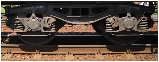
Figure 1.
Y25 bogie side view.
The additional technical aim of this paper can be formulated as confirming or refuting the accusations made against the Y25 bogie about its poor running performance. The primary suspension parameters were changed to check the potential to improve the bogie behaviour.
1.1. The Literature Survey
The papers in which problems on railway vehicles’ stability, including determination of their nonlinear critical velocity vn, are discussed by the present authors are [5,6,7]. Broad reference to the corresponding literature by other authors is provided in these publications, too. The newest examples of papers discussing the stability and dynamics of rail vehicles, also with their motion on CCs and TCs taken into account, are [8,9,10,11,12,13,14,15,16,17,18,19,20,21,22,23,24]. In [8], its authors study the stability of high-speed trains through a focus on bogie behaviour. A novel method for stability determination, based on root loci methods, is successfully tested. A sensitivity analysis was performed on the selected vehicle parameters, too. In [9], one can see the interesting differences in stability issues for rail and road vehicles. The important influence of the vehicle roll angle on stability is considered. The results on the stability region are presented as a three-dimensional stability domain. Paper [10] describes a novel measuring system that monitors vehicles’ hunting motion. Based on the monitoring results, the system can predict the lateral and yaw displacements of the wheelset and the contact relationships for the wheel–rail pair in real time. The accuracy and efficiency of the whole system were validated by comparing the predicted results with simulated and experimental results. Paper [11] is truly interesting and of high intellectual value. It reveals and verifies experimentally (on a roller rig) the possible existence of parametric vibrations in a wheelset–track system. They appear parallel to self-exciting vibrations (hunting motion) and are caused by wheel load fluctuations. Systems particularly prone to this type of resonance are those with large tread angles, which also decrease the critical (hunting) velocity, favouring the simultaneous existence of self-exciting and parametric vibrations. Publication [12] represents a study of the chaos in a mechanical impacting system. The novelty of this paper lies in the extension of previous results for a one-degree-of-freedom (DoF) system to a two-DoFs system. The existence of phenomena such as narrow-band chaos, finger-shaped attractors, etc., was demonstrated numerically and then experimentally verified. In [13], the authors propose a new method for stability determination based on data instead of equations. With this method, they managed to determine the long-term statistics of the chaotic state, the covariant Lyapunov vector, the Lyapunov spectrum, the finite-time Lyapunov exponents, and the angles between the stable, neutral, and unstable splitting of the tangent space [13]. Publication [14] presents and uses one more nonlinear wheelset model to perform bifurcation analysis. The nonlinearity in the wheel–rail contact is of primary interest. The analysis comprises comparisons between the results for linearised and nonlinear models. The results for different field-measured wheel profiles are also compared. Finally, the conclusion is that a greater suspension stiffness increases the stability under wheel wear conditions. Publication [15] is to some extent similar to [14]. A nonlinear wheelset model undergoes bifurcation analysis. The nonlinear equivalent conicity in wheel–rail contact is of interest. The results for linear and nonlinear approaches to equivalent conicity and contact forces are compared. The authors show the possible coexistence of stable and unstable limit cycles and expand on the consequences of Chinese high-speed trains’ observed unfavourable behaviour. In paper [16], the authors study the influence of the curved track parameters, such as their radii, superelevation, and TC and CC lengths, on vehicle–track interactions in the case of a side-frame cross-braced two-axle railway bogie. They conclude that the curve radius is of unequivocal importance, the TC length is important provided the inflection point is not exceeded, superelevation is of minor importance (the differences in the results for the superelevation deficiency and excess are surprisingly small), and the CC length is of no importance at all. In [17], the authors focus on vibrations in passenger cars. They compare results from two approaches, one based on analytical solutions to dynamical equations and the other based on simulation, which means solving the equations numerically. Thanks to the greater DoFs possible and less simplification of the equations with the simulation approach, the authors conclude that it is superior to the other approach. The authors highlight the higher accuracy of the simulations. Publication [18] compares a few methods for nonlinear critical velocity determination. A simulation approach to this issue and ramping and path-following (continuation) methods are of primary interest. Different methods for hunting motion excitation are compared with each other in terms of the critical velocity value. The impact of the track class (its irregularities) on the results is also shown thanks to comparison with the results for an ideal track. In [19], the effect of the bogie’s parameters in suspension on the lateral forces in the track frame is studied. This bogie is a three-piece traditional construction applied in freight cars. The authors consider 30 different bolster suspension combinations. It is concluded that an increase in the dumping force (the friction coefficient of the wedge) causes an increase in the lateral force of the track frame. Simultaneously increasing the bogie’s lateral stiffness and the dumping force raises the lateral force of the track frame, too. On the other hand, the internal interplay between these two parameters also appears important. In [20], the hunting motion of a locomotive car body is studied experimentally and according to simulation. The aim is to explain and suggest measures to eliminate such hunting motion that appears for low conicity in wheel–rail contact. The measures concern the suspension parameters. Namely, the series stiffness and damping in the yaw damper and the longitudinal stiffness in the primary suspension are indicated as those that need to be decreased. Both ST and CC cases are analysed. In paper [21], the author studied interactions between a vehicle’s internal elements and between the vehicle and the track to make sure that existing freight cars with three-piece bogies can run at higher permissible speeds under an increased axle load. ST and CC sections are considered. It is shown that such increases are possible. However, the bogies have to be replaced with slightly modernised ones. In [22], the authors propose a method to identify, rather than neglect, low-amplitude hunting in high-speed railway vehicles. They found that the coefficient of autocorrelation and the spread of spectral frequency are the most efficient parameters for this purpose. The findings are dedicated to supporting the monitoring of hunting motion instability and active control studies for high-speed trains in real time. Paper [23] is a general paper on the instability of limit-cycle-type oscillations. The aim is to derive an efficient computational method for instability modelling and handling hundreds, sometimes thousands, of design variables. This is fulfilled by using a simple metric to determine the stability of the limit cycle utilising a fitted bifurcation diagram slope. Stability derivatives for many design variables are efficiently computed using the developed adjoint-based formula. Publication [24] proposes a nonlinear wheel–rail kinematics model, which extends Klingel’s well-known linear model. The nonlinear model comprises high-order odd harmonic frequencies (HOHFs) [24], besides the basic hunting frequency. Along with this, HOHFs are sources of self-exciting vibrations in rail vehicles. Thus, these findings are important to the methods in hunting instability research and condition monitoring for trains.
Summarising the content of these publications, one can note that their scope is similar to that of the profiled literature from 15 years ago. So, we find works of intellectual quality, works on new methods of research and description, and works on general dynamics, stability issues, hunting (limit cycles), chaos, and so on. Yet there are many more works concerning issues for STs than those for CC and TC problems.
1.2. The Fundamental Theoretical Considerations
Although part of the discussed literature directly concerns stability issues, the fundamentals of stability are given below.
The physical explanation for practical problems with rail vehicle stability is the self-exciting vibrations that appear in vehicle–track systems. This phenomenon has been recognised for a long time [25]. Some vehicle parts undergo self-exciting vibrations under certain motion conditions (parameter values). The wheelsets oscillate laterally and around the vertical axis (yawing). Wheel flange–rail contact, noise, and a higher risk of derailment accompany this. Although a vehicle’s motion along the track is usually possible under such conditions, self-exciting vibrations cause obvious adverse phenomena in rail vehicle operation in straight track (ST) and circular curve (CC) sections. The self-exciting vibrations observed in real vehicle–track systems [25] can be identified using vehicle–track models with bifurcation of the solutions [26,27]. Bifurcation analysis is an effective method for testing modelled objects [26,27,28,29] and is thus applied also in the presented research. Numerical simulation studies on vehicle–track systems enable us to observe whether the model solutions are stable. Stable stationary solutions (with constant values of the model’s observed coordinates on STs and CCs) describe the normal exploitation conditions for a real vehicle. This means that in the real system, each disturbance, for example, disturbance caused by track irregularities, is effectively damped, while the system tends toward equilibrium. A properly designed vehicle should ensure running stability in the expected range of exploitation parameter changes, such as velocity (0 to vmax), load (empty or partially to fully loaded), load asymmetry, track shape (CC, transition curve (TC), ST), track maintenance, etc. Stable stationary solutions for a modelled vehicle–track system on STs and CCs are expected under typical operation conditions. In contrast, due to the constant change in the curve radius and superelevation on TCs, stationary solutions for TCs are neither possible nor expected.
The model’s stable periodic solutions (limit cycles) are attributed to self-exciting vibrations in the real system. Due to them, the lateral displacements in the wheelset change periodically during the main vehicle motion (along the track). Calling such solutions “stable periodic” is justified because they are limited and observable and can last any length of time. On the other hand, stable periodic solutions represent the highest capacity of the modelled system in terms of stable behaviour and also bring other valuable information. The key parameter in stability analysis is nonlinear critical velocity vn, as well as in the present research. The value of vn separates the range of vehicle velocity v for which stable stationary solutions exist (v < vn) from the range for which stable periodic solutions may appear (v ≥ vn). The value of vn is the minimum vehicle velocity v starting from which stable periodic solutions can exist. For a real object, this means self-exciting vibrations may occur, and a vibrational system state is reached. Further increase in the system output (for example, with a rise in v) leads to an increase in the self-exciting vibration amplitude. Finally, the amplitude values are no longer constant, which causes unbounded growth of the solutions (a loss of stability), which could lead to an accident due to the derailment in the real system. The research on periodic solutions for vehicle models under increased system input (vehicle velocity) in an above-critical system state is interesting. It is conducted to ascertain how much the system parameters (velocity) can be exceeded and the solutions still kept stable (periodic or stationary). A wide range of system velocities between the values corresponding to the appearance of periodic solutions and a loss of stability is always desirable for a real vehicle.
2. The Approach to Stability and the Corresponding Model
The stability studies discussed in the present paper, originating from the project specified in the Acknowledgements section, represent, according to a general view, the bifurcation approach to stability. Within it, a simulation method for studying nonlinear lateral stability is applied. Such a method is beneficial when considering rail vehicle systems (vehicles) and their entire dimensions, when one prefers to consider the entire system’s degrees of freedom (DoFs) rather than considering one or two degrees of freedom for a single wheelset. The latter may be an alternative for some authors. Its advantage is the use of analytical methods. These can be applied to small systems only. At the same time, numerical simulations are helpful no matter what the dimensions of a given system are.
On the other hand, authors have used an original approach with the method of studying the lateral stability on CCs, as elaborated in [5,6]. With this method, an ST is taken as a CC with an infinite curve radius of R = ∞. Vehicle velocity v is typically the bifurcation parameter, as it is here. The authors’ original bifurcation diagrams are utilised, providing a convenient form for presenting the results. These diagrams are bipartite, where the maximum absolute value of the leading wheelset’s lateral displacements |ylw|max versus velocity and the peak-to-peak value of ylw versus velocity [5,6,7] are represented correspondingly. When jointly presenting these coupled values for all the radii values R, one obtains two complex bifurcation diagrams. The authors call such a pair of bifurcation diagrams a stability map [5,6]. The first stability map in this paper is Figure 5, which can serve as an example.
Following the bifurcation approach and their method, the authors needed simulation models for a whole vehicle with many DoFs for their studies. Consequently, a rail vehicle model with Y25 bogies was also created and tested. As mentioned before, its first wheelset’s lateral displacements ylw were chosen for observation. In fact, a model of the whole vehicle–track system was created. The authors used the VI-Rail engineering software for this task. In it, type I Lagrange equations are used to build equations of the system dynamics. All the inertia terms for motion on a curved track are taken into account. The main nonlinear elements within the models are those arising from the nonlinear kinematics in the curved tracks, the nonlinear contact geometry, and the nonlinear contact forces in the wheel–rail pair. The suspension parameters were assumed to be linear. The VI-Rail software is a well-established commercial product of high credibility. Nevertheless, the authors verified it when the project mentioned in the Acknowledgement section was realised. This was a kind of benchmarking approach. The simulation results from the commercial software were contrasted with the results from software built by the authors, according to which complete insight into the program code was made possible. The results of these comparisons appeared satisfactory.
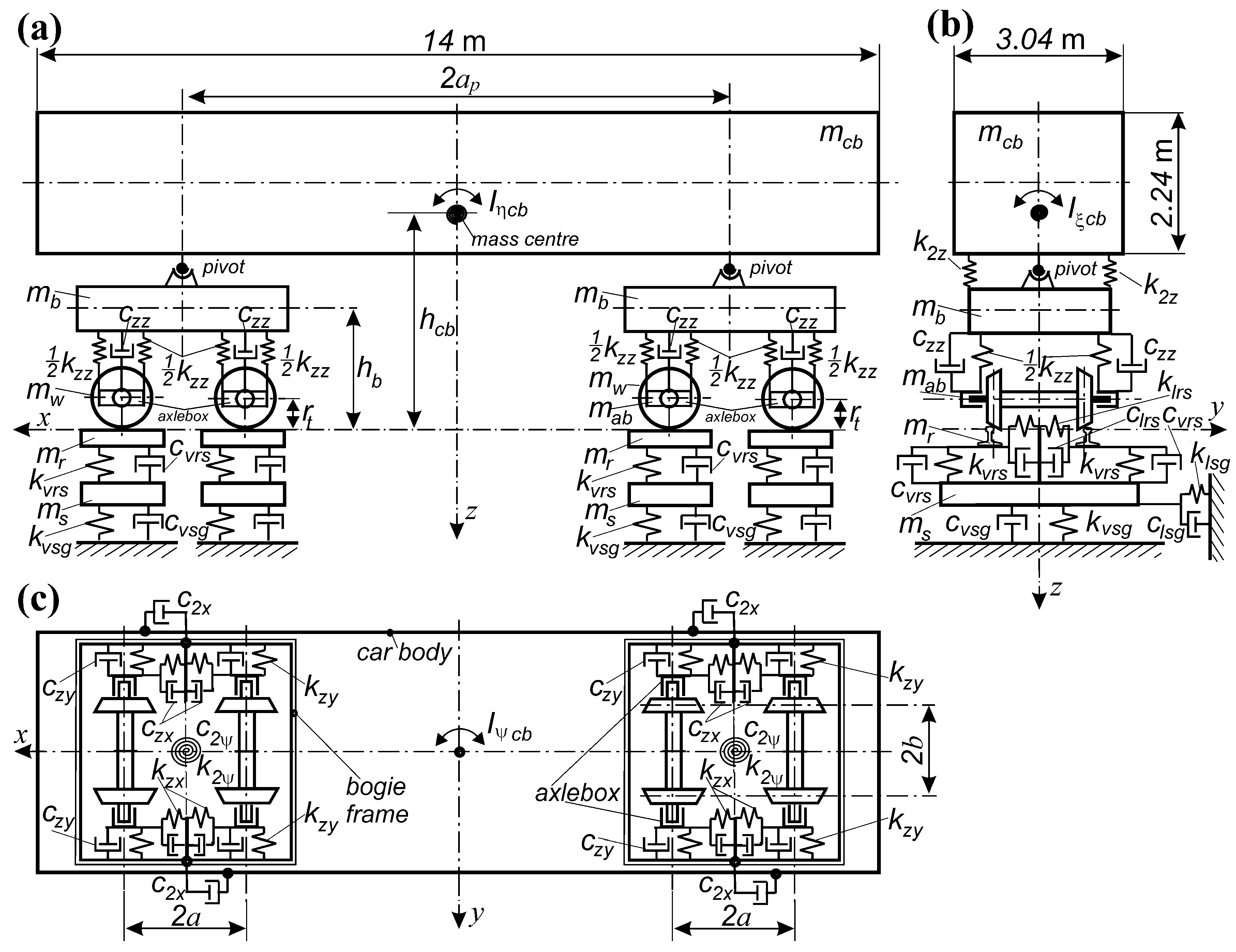
The model built is a discrete model of a cargo gondola car type 412W Eaos (see Figure 2). Its bogie models represent a Y25 construction (alternatively named 25TN in Poland). A total of 15 rigid bodies make up the model of the 412W gondola. These are a loading space (a gondola), two bogie frames, four wheelsets, and eight axle boxes. The connections between the rigid bodies are flexible elements, with linear and bi-linear characteristics for stiffness and dumping. The suspension structure of the Y52 bogie comprises dry friction dampers. However, in order to avoid the non-smooth problem in modelling dry friction (stick–slip effect in the suspension), viscous dampers are applied in the model. Furthermore, each dry friction damper in the Y25 bogie acts vertically and laterally. Thus, to describe the damping forces, a two-dimensional model of dry friction should be considered [30,31,32]. A pair of individual viscous dampers acting vertically czz and laterally czy are finally adopted to simplify the bogie model. Vertical coil springs (formed as two-spring sets) in each axle box represent the stiffness in the vertical kzz and lateral kzy directions. The parameters of stiffness and damping just mentioned take two values each. One refers to empty gondola conditions and the second to laden gondola conditions (see Table A1 in Appendix A). In this simple way, the dependence of the parameters on the vertical load is considered to some extent. The values of the stiffness and damping parameters were obtained following the identification procedure performed at the authors’ home faculty [33]. Experiments on a real freight car with Y25 bogies were its basis. Shortly, for the damping, the measured car’s responses enabled formulae for vertical and lateral damping forces to be built and then the linear equivalent coefficients for different discrete car load states in the indirect procedure to be determined. The result is somewhat simplified. Nevertheless, the procedure is multi-level and scientifically advanced.
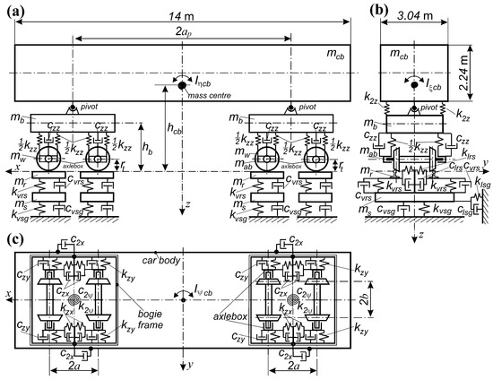
Figure 2.
Nominal model of the 412W gondola–track system: (a) side view, (b) front view, (c) top view.
On the other hand, the literature shows that damping forces can be crucial to vehicle dynamics. An example is a recent vertical dynamics study [34] for high-speed rail where comfort issues for vehicles running up to 400 km/h on a track with vertical irregularities were tested. It confirmed that when considerable vertical dynamical interactions between the vehicle and the track exist and are of interest, the influence of the vertical load on the damping forces (dry friction dampers) should be as accurate as possible. The conditions in the present study are different, however. The vertical dynamics is out of scope, while the vehicle’s admissible speed vad = 120 km/h. Equally, the track is perfect, which means no vertical or lateral irregularities are considered. Consequently, vertical load changes (influencing forces for the dry friction damper laterally and vertically) almost do not exist. Additionally, in such circumstances, the well-known and commonly applied assumption easily holds that the couplings between the rail vehicle’s lateral and vertical dynamics are insignificant. Then, analyses can be carried out separately for the lateral and vertical directions, e.g., [10,14,15,24,33,34]. In practice, no mutual influences of vertical and lateral dynamical solutions can be observed. Thus, the simplified modelling of vertical dumping does not influence the lateral dynamics (lateral stability) in the present study.
The longitudinal guidance of the wheelsets is very stiff. It represents a type of horn guidance [28]. So, eventual small deflections in the guide’s material only effect the longitudinal stiffness kzx. Because of this, it is agreed that kzx is independent of the car load.
The freight car model is supplemented with a flexible track model, both vertically and laterally. The track parameters correspond to a ballasted European track with a 1435 mm gauge. Nominal profiles of UIC60 rails with an inclination of 1:40 are adopted. Nominal profiles of S1002 wheels are taken. The parameters of nonlinear wheel–rail contact are calculated using the ArgeCare RSGEO software. The tangential forces in the wheel–rail contact are calculated using Kalker’s simplified theory, implemented in the FASTSIM numerical procedure [35,36]. Integration of the equations of motion is performed using Gear’s procedure. The error and step size control characterise its features. Its suitability for solving stiffness problems is well known, as with rail vehicle dynamics issues [28,29]. The whole model of the vehicle–track system possesses 76 kinematic DoFs. Appendix A (Table A1) comprises detailed parameter values for the whole model.
3. The Method of Research
Analysis of car model solutions, performed for the range of velocity v and its constant value in each simulation, is the essential element in the authors’ research method. To explain the wheelset oscillations (its hunting motion), the theory of self-exciting vibrations is used. The range of vehicle velocity v starts, e.g., at 10 m/s, while its end is determined by the maximum value at which stable solutions of the model still exist. Generally, the model parameter observed in studies is the leading wheelset’s lateral displacement ylw in time or distance. The term stable solution is adopted when describing the ylw solutions for constant or periodic (of a limit cycle nature) values. The same criteria for a stable solution on STs and CCs hold in the analyses discussed in this paper. Different from the mentioned forms of solutions are those classified as unstable, although they may fulfil other stability criteria, e.g., technical stability [37].
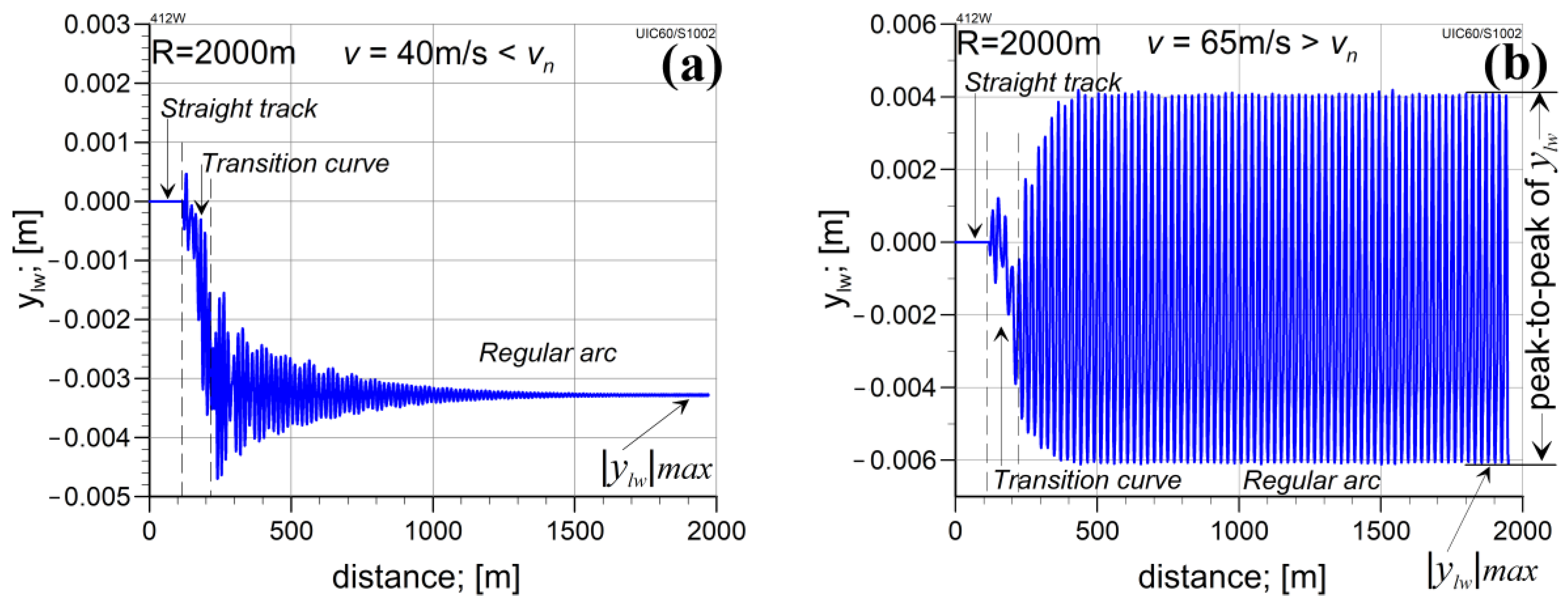
Example stable solutions, typical for vehicle motion velocity lower than the critical value (v < vn) and above than critical value (v > vn), are shown in Figure 3a,b, respectively. The vehicle motion in this example takes place on a route composed of ST, TC, and CC sections. The CC’s radius R = 2000 m. The wheelset undergoes a lateral shift while negotiating the TC; thus, ylw ≠ 0 on the regular CC. The track’s superelevation influences it also. The superelevation values h applied to the CC tracks for the studied R values are shown in Table 1. The h values are constant during the calculations on the CCs for each radius R. That means that at lower speeds, excess superelevation (cant) exists, while at higher speeds, insufficient superelevation (cant) exists. To be precise, the superelevation values provide an ideal balance between the lateral components in the track plane of centrifugal and gravity forces at v = 34.29, 41.23, 46.45, 44.90, and 44.77 m/s for R = 1200, 2000, 3000, 4000, and 6000 m, respectively.
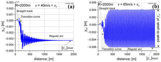
Figure 3.
Example lateral displacements ylw of the first wheelset as a function of distance: (a) stable stationary solution (40 m/s < vn); (b) stable limit cycle (periodic solution, 65 m/s > vn).

Table 1.
The tested curve radii and corresponding track superelevations.
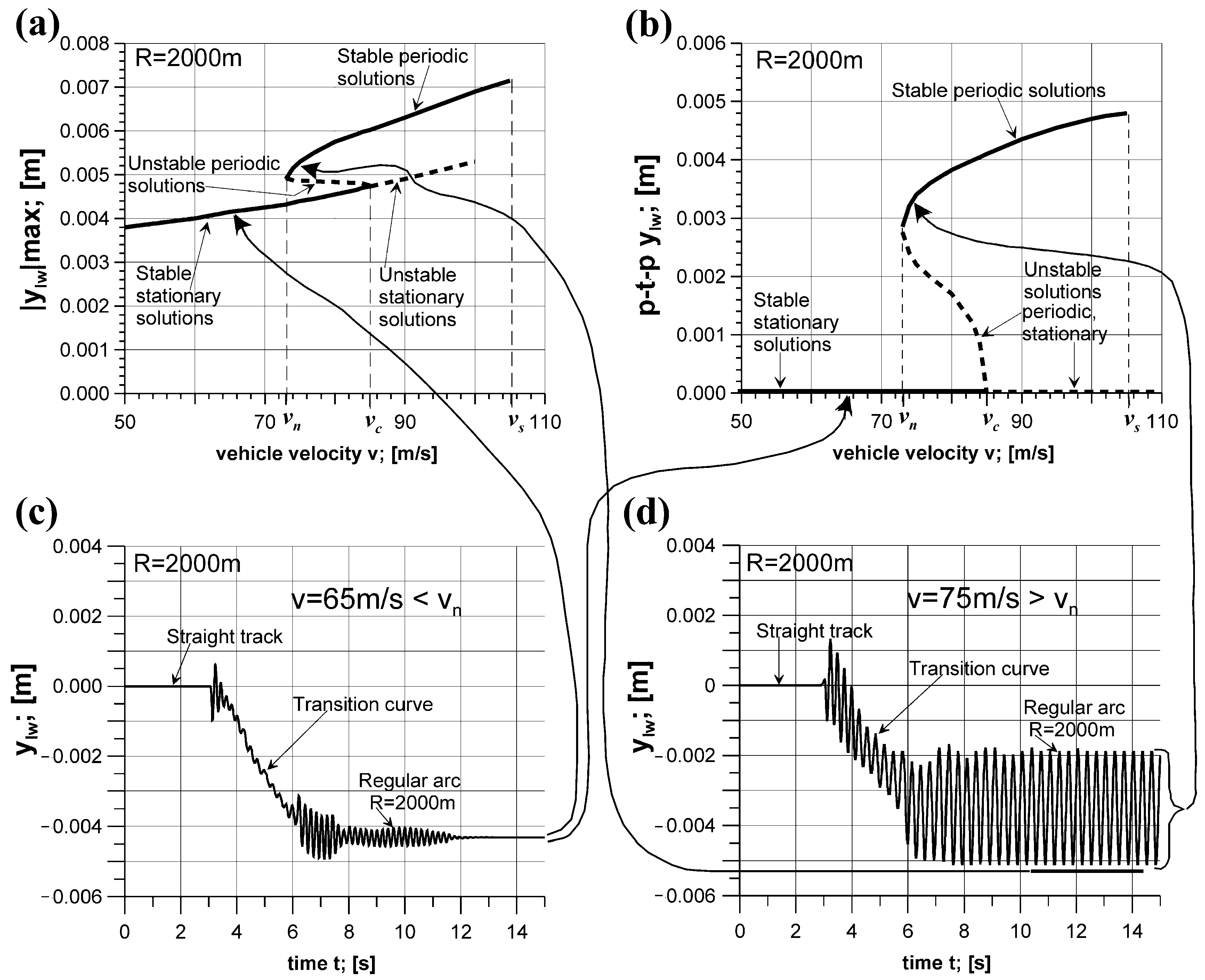
The studies in [6] and the present research demonstrate that the wheelset’s oscillations are a limit cycle, described as that of hard excitation. In other words, initial conditions of a given minimum value must occur for vibrations to start. When studying the stability of the model on CCs, the negotiation of the TC forces a lateral shift in the wheelset on the track, which means it falls out of equilibrium. This way, non-zero initial conditions for solutions on CCs are imposed. For the stability analysis on an ST, a single lateral irregularity in the track serves as the input (equivalent to the initial conditions). Usually, it is located 100 m from the beginning of the test route. Thanks to the negotiation of the irregularity, lateral shifts in all the wheelsets take place one by one. The shifts adopted are typically between 0.005 and 0.006 m. After each simulation, the maximum value of the lateral displacement of the leading wheelset in the first bogie ylw max has to be read from the final part of the simulation results. ylw max can be positive or negative (as in Figure 3), depending on the coordinate system orientation and the curve direction. When the curve turns to the left, this corresponds to a negative value. Actually, the simulation solutions for left- and right-hand side curve turns are antisymmetric to each other when the same conditions of motion occur. This enables us to avoid the problem of the sign. We can use the maximum absolute value of the wheelset lateral displacements |ylw|max instead of ylw max. This quantity ultimately represents the simulation solutions for a particular velocity v. In the case of a stationary solution (Figure 3a), |ylw|max is the only recorded value for the solution. An additional quantity is read off and recorded for a periodic solution (Figure 3b), namely the peak-to-peak value of ylw. The peak-to-peak value of ylw = 0 in the case of stationary solutions. Consequently, |ylw|max and the peak-to-peak (p-t-p) value of ylw for each simulation for a constant velocity v and radius R are read off and recorded, forming a pair of bifurcation plots. Such pairs are presented jointly for all R values to create stability maps. The way stability maps are built is shown in Figure 4, however, for just one selected value of R = 2000 m. Each of the simulations, as in Figure 4c,d, produces one point on the whole courses shown in Figure 4a,b. These points correspond to the velocities v for which the simulations in Figure 4c,d were performed. Simulations for the whole range of velocity v must be performed to ascertain the whole course. In the same way as in Figure 4, courses for other R values are obtained. As already explained, a stability map is built as a pair of joint bifurcation diagrams representing |ylw|max and the p-t-p value of ylw (p-t-p ylw for short) as a v function for CCs of different radii R. The first stability map in this paper is Figure 5. The map components (here, Figure 5a,b) enable us to observe the solutions’ nature, the solutions’ values, and the critical velocity vn values in the v range within which stable solutions exist. For the existing stationary solutions exclusively, especially for the range of v below vn, the results start to be presented from v just below the value of vn (usually about 30 m/s in this study). Then, they are continued for the entire range of velocities above the critical value. The courses on the diagrams are marked with different line colours, referring to a specific constant radius R of the CC route. The last points on the courses represent the highest velocity at which a stable solution (no matter whether stationary or periodic) still exists. Examples of stability determination on the part of the authors are given in detail in [5,6,7].

Figure 4.
The idea of building a pair of bifurcation plots and the component elements of a stability map [7] for a CC with R = 2000 m: (a) example simulation of stationary solution on CC; (b) example periodic solution for CC; (c) bifurcation plot of |ylw|max; (d) bifurcation plot of p-t-p ylw.
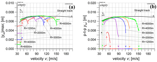
Figure 5.
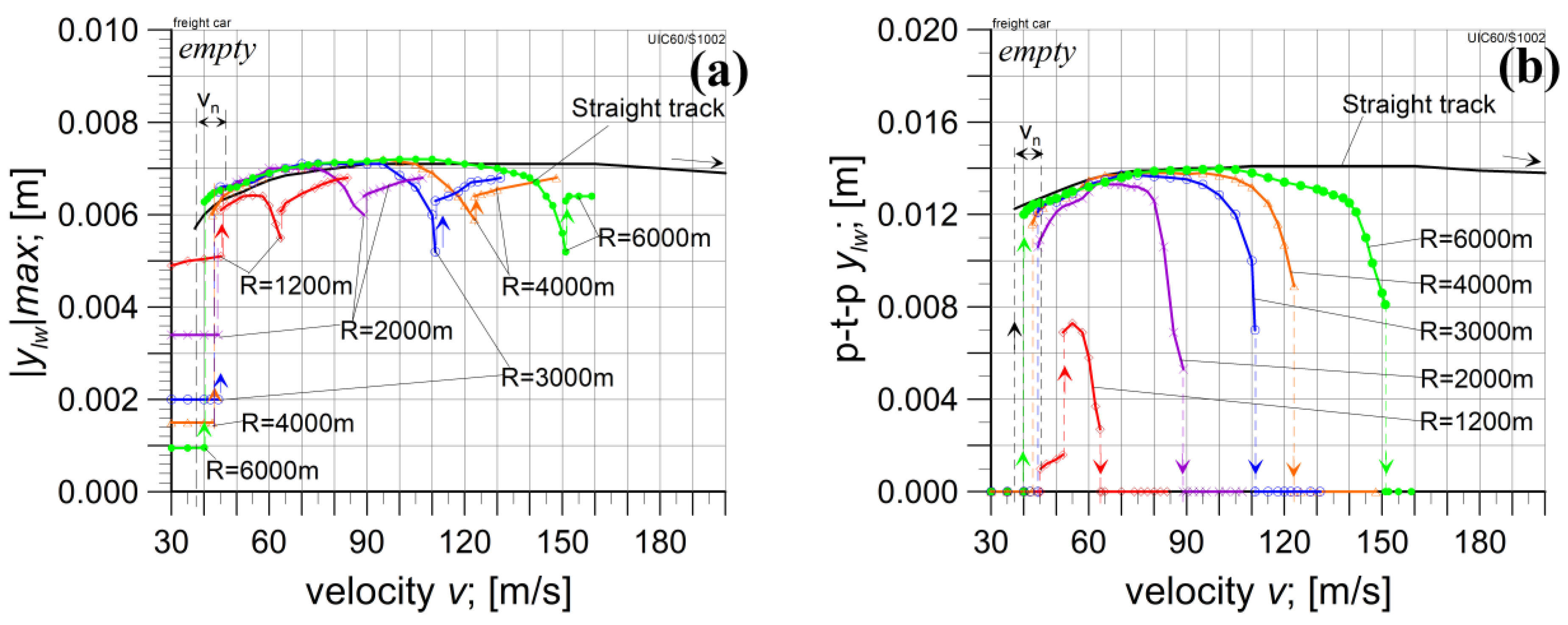
Stability map of an empty gondola car: (a) absolute value of the leading wheelset’s maximum lateral displacement |ylw|max; (b) p-t-p value of ylw as a function of vehicle velocity.
4. Results of the Research
4.1. The Empty Car Analysis
Stability maps for the motion of an empty wagon model are shown in Figure 5. As can be seen there, the properties of the model are regular. That is, for each of the tested routes, the critical velocities vn were determined. Only stable stationary solutions appear for velocities lower than the critical value. Periodic solutions exist for velocities equal to and higher than the critical value vn. The values of the critical velocity vn on each curved track increase as the curve radius decreases (Table 2). The smallest value is 37.2 m/s for an ST (R = ∞), and the highest vn is 45.2 m/s for a CC with R = 1200 m. Stable periodic solutions still exist at velocities greater than 200 m/s on the ST (black line). The velocity ranges where periodic solutions for CCs occur are smaller than those for STs and decrease as the curve radius decreases (different line colours for particular R values). For each CC section and the final range of velocities, there is a bifurcation of periodic to stationary solutions, which are the stable ones. Potentially, this could be the effect of the action of centrifugal force. Only stable stationary solutions exist in the range of velocities lower than the critical value, with the |ylw|max values increasing as the curve radius decreases. Therefore, the diagrams show results for a motion velocity higher than 30 m/s. The wheelsets not being centrally located on CCs below vn (|ylw|max ≠ 0) results from the motion conditions, including the applied superelevation of the track (Table 1).
Table 2.
The nonlinear critical velocity values vn of the modelled gondola car.
So, in light of the tests carried out on the car model in an empty state, the requirements regarding motion stability for operating velocities (less than 120 km/h ≈ 33.33 m/s) are met. The critical velocities on particular tested routes are not lower than the maximum operational velocity. Periodic solutions with |ylw|max values up to approximately 0.006 to 0.007 m appear for the critical and greater than critical velocities. This means that self-exciting vibrations of the wheelsets may occur in the modelled system. Still, the basic motion of the vehicle (along the track) is also possible at a velocity over the critical value.
4.2. Loaded Car Analysis
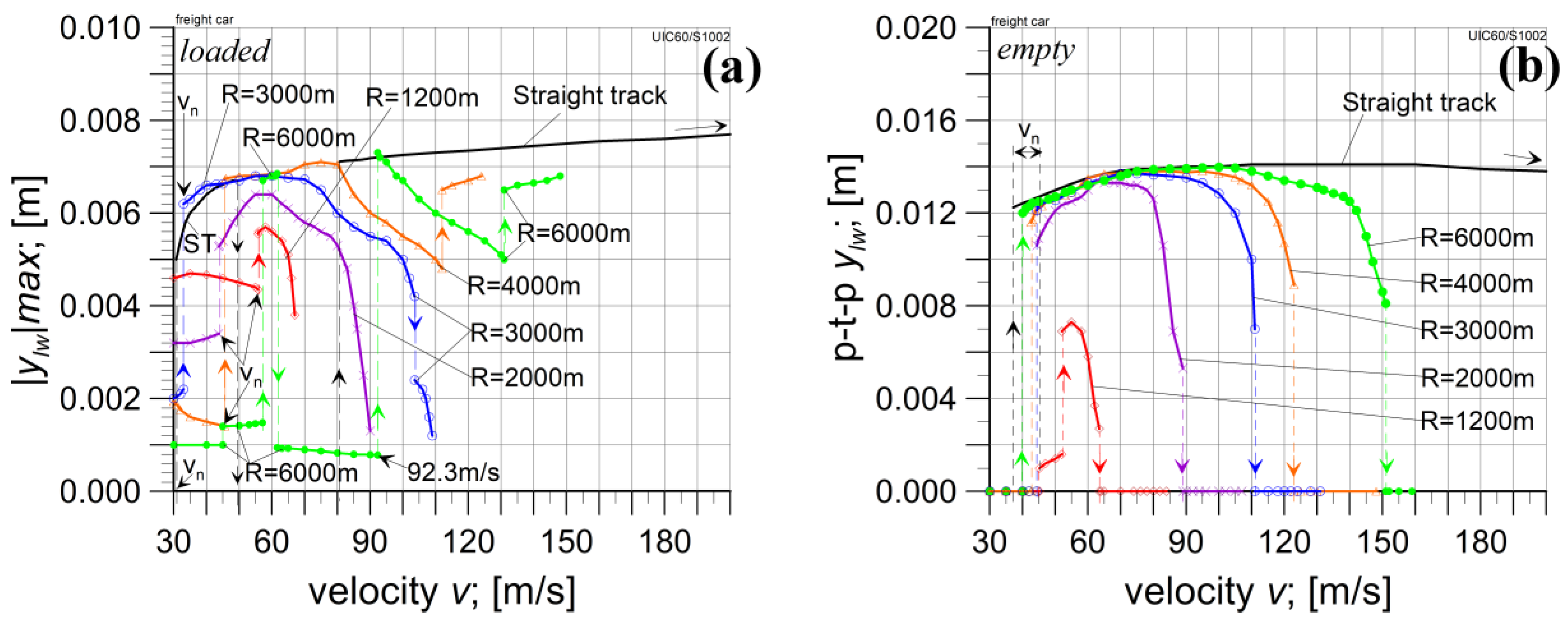
The laden vehicle model presents significantly different features under the same motion conditions (track curvatures, Figure 6) from those of the empty one. Motion on an ST represents the lowest value of critical velocity vn = 30.8 m/s. This value is below the vehicle’s maximum operating (admissible) velocity vad = 120 km/h ≈ 33.3 m/s. This means self-exciting vibrations may appear in the modelled car during regular operation. Critical velocities are higher on CCs (Table 2) than on STs. In the range of velocities over the critical value, the solutions are bifurcated from periodic to stationary and from stationary to periodic on an ST and a CC with R = 6000 m. These make the stability maps hardly legible. Therefore, analyses of selected solutions on the routes for a loaded car are presented in separate diagrams further on.
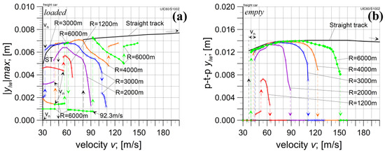
Figure 6.
Stability map of laden gondola car: (a) maximum absolute value of the leading wheelset’s lateral displacement |ylw|max; (b) p-t-p value of ylw as a function of vehicle velocity.
4.2.1. Analysis on a Straight Track
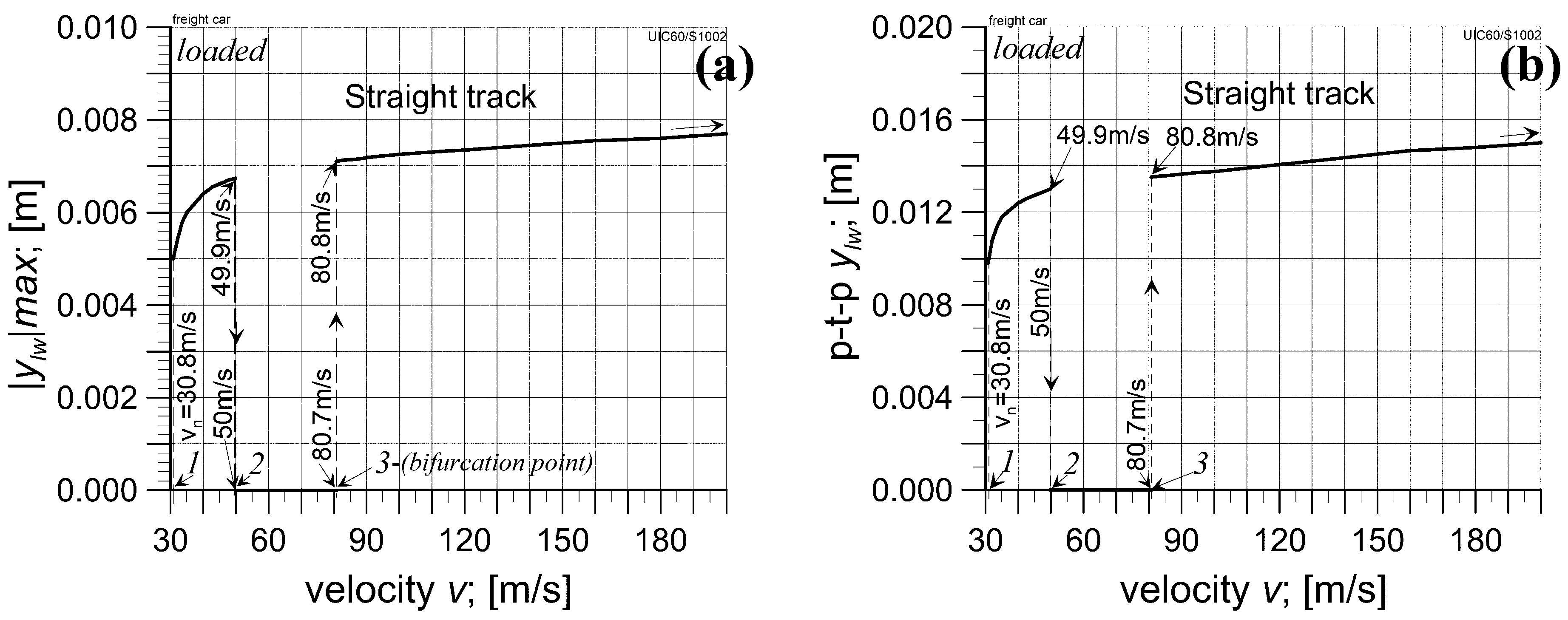
The periodic solutions that appeared on the ST at 30.8 m/s exist until the velocity v equals 49.9 m/s (Figure 7). Increasing v over this value by 0.1 m/s causes the bifurcation of periodic solutions to stationary ones. Stationary solutions persist up to a v value of 80.7 m/s. Increasing the velocity v by 0.1 m/s further causes bifurcation to periodic solutions again. The periodic solutions last until the end of the tested velocity range (200 m/s).
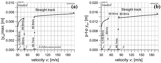
Figure 7.
Loaded car stability map on an ST. The nominal value of lateral stiffness applied kzy = 55.6 ∗ 105 N/m: (a) maximum absolute value of leading wheelset’s lateral displacement |ylw|max; (b) peak-to-peak value of ylw versus vehicle velocity.
Next, research was undertaken to eliminate the possibility of the occurrence of periodic solutions (self-exciting vibrations in real systems) in the modelled car’s operating velocity range. Elements of the suspension system have a crucial impact on the dynamic properties of the vehicle. Changing the suspension parameter values is usually a relatively simple process. Accordingly, the influence of the longitudinal and lateral stiffness (kzx, kzy) and damping (czx, czy) on the primary suspension was examined by varying their values. The result of these tests is the determination of the lateral stiffness kzy parameter for which a drop in value compared to the nominal value gives the most favourable effects, i.e., improvements in the analysed car’s properties. The test results are shown in Figure 8.

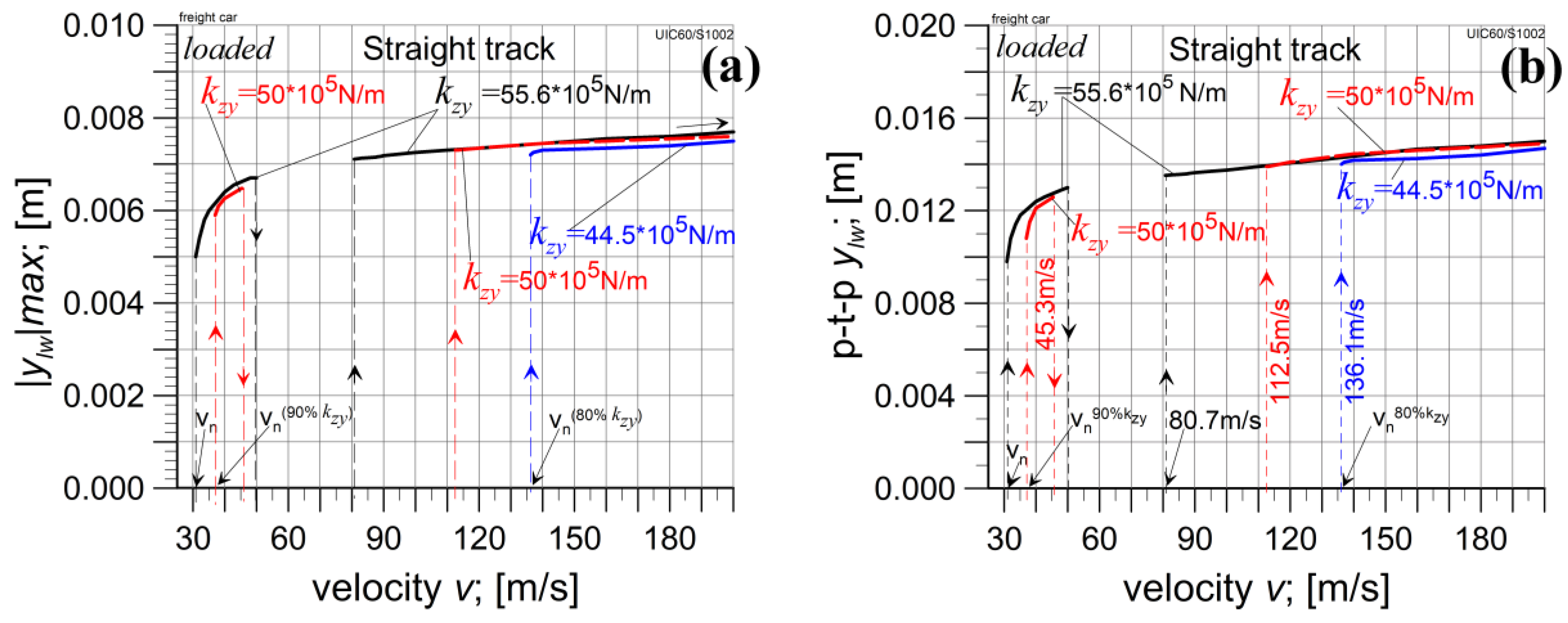
Figure 8.
Influence of the lateral stiffness kzy on laden car’s first wheelset. kzy = 55.6 ∗ 105 N/m—nominal value (black line), kzy = 50 ∗ 105 N/m—90% of nominal value (red line), kzy = 44.5 ∗ 105 N/m—80% of nominal value (blue line). Motion on the ST: (a) maximum absolute value of lateral displacement; (b) peak-to-peak value of wheelset’s lateral displacement.
A reduction in the lateral stiffness to 90% of its nominal value (90% ·kzy = 0.9·55.6·105 ≈ 50·105 N/m) increases the vn velocity up to 36.9 m/s. At this velocity, periodic solutions appear and exist up to 45.3 m/s. Then, bifurcation from periodic to stationary solutions in velocity v cause bifurcation from stationary to periodic solutions, with values close to those obtained for the nominal value of kzy. Periodic solutions persist up to velocities exceeding 200 m/s. A further decrease in the lateral stiffness value, down to 80% of the nominal value (80% · kzy = 0.8·55.6·105 ≈ 44.5·105 N/m), causes a jump in the critical velocity value. In this case, the range of periodic solutions which existed at velocities lower than 50 m/s disappears. Stationary solutions exist for a velocity of up to 136.1 m/s. Then, bifurcation to periodic solutions occurs. The values of the solutions are similar to those determined at the nominal value of the lateral stiffness. This type of solution lasts up to v = 200 m/s. So, a decrease in lateral stiffness kzy by a dozen percent relative to the nominal kzy value enables an improvement in the stability properties of the loaded car on an ST.
4.2.2. Analysis on Curved Tracks
The following step in the research examined whether the beneficial effect on an ST (regarding the improvement in the system properties) due to reducing the lateral stiffness kzy would also appear as a favourable improvement on a CC with R = 6000 m. For the nominal value kzy = 55.6·105 N/m, the corresponding critical velocity was vn = 45 m/s (Figure 9). This was determined to be to some extent arbitrary because at a lower v value (about 20 m/s), “periodic” solutions of the minimal p-t-p value of ylw appeared. A velocity vn = 45 m/s was adopted, judging that the p-t-p value of ylw was large enough (about 0.001 m) at this velocity to talk about periodic solutions in the practical sense. However, a considerable increase in the p-t-p value of ylw to a dozen millimetres is observed at a velocity of 57.1 m/s. Stable periodic solutions exist up to v = 61.6 m/s only, thereafter being replaced by bifurcation to stationary solutions. In further increasing the velocity, stationary solutions exist up to 92.3 m/s. Then, bifurcation to stable periodic solutions is observed. Periodic solutions exist until v = 131 m/s. Next, bifurcation to stable stationary solutions appears. Such solutions exist for a high velocity range from 131 to 148 m/s. At even greater velocities, no stable solutions are observed.
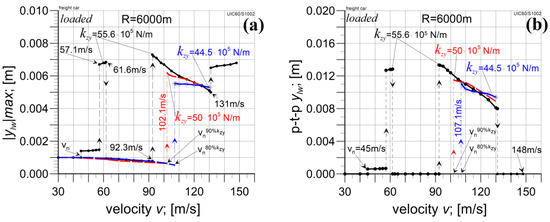
Figure 9.
Influence of lateral stiffness kzy on laden car’s first wheelset. kzy = 55.6 ∗ 105 N/m—nominal value (black line), kzy = 50 ∗ 105 N/m—90% of nominal value (red line), kzy = 44.5 ∗ 105 N/m—80% of nominal value (blue line). Motion on CC of R = 6000 m: (a) maximum absolute value of lateral displacement; (b) peak-to-peak value of wheelset’s lateral displacement.
In the following research step, the lateral stiffness decreased to 90% of its nominal value, kzy = 0.9·55.6·105 ≈ 50·105 N/m. Stable stationary solutions persist up to v = 102 m/s. Similarly to the model with a nominal value for lateral stiffness, some “periodic” lateral displacements of the wheelset appear on the curve, too. Nevertheless, they have minimal p-t-p values. Increasing the vehicle velocity to v = 102.1 m/s induces bifurcation to periodic solutions. This type of solution persists when increasing v up to 131 m/s.
The next step was reducing the lateral stiffness to 80% of its nominal value (80% · kzy = 0.8·55.6·105 ≈ 44.5·105 N/m). Stable stationary solutions occur up to a velocity v = 107.1 m/s. Bifurcation from stable stationary solutions to stable periodic one occurs at this velocity. Periodic solutions last up to approximately v = 130 m/s. The values of |ylw|max and p-t-p ylw for all the kzy values tested are similar. To conclude, a reduction in the lateral stiffness kzy by a dozen percent compared to its nominal value results in a considerable rise in the critical velocity on a CC of R = 6000 m.
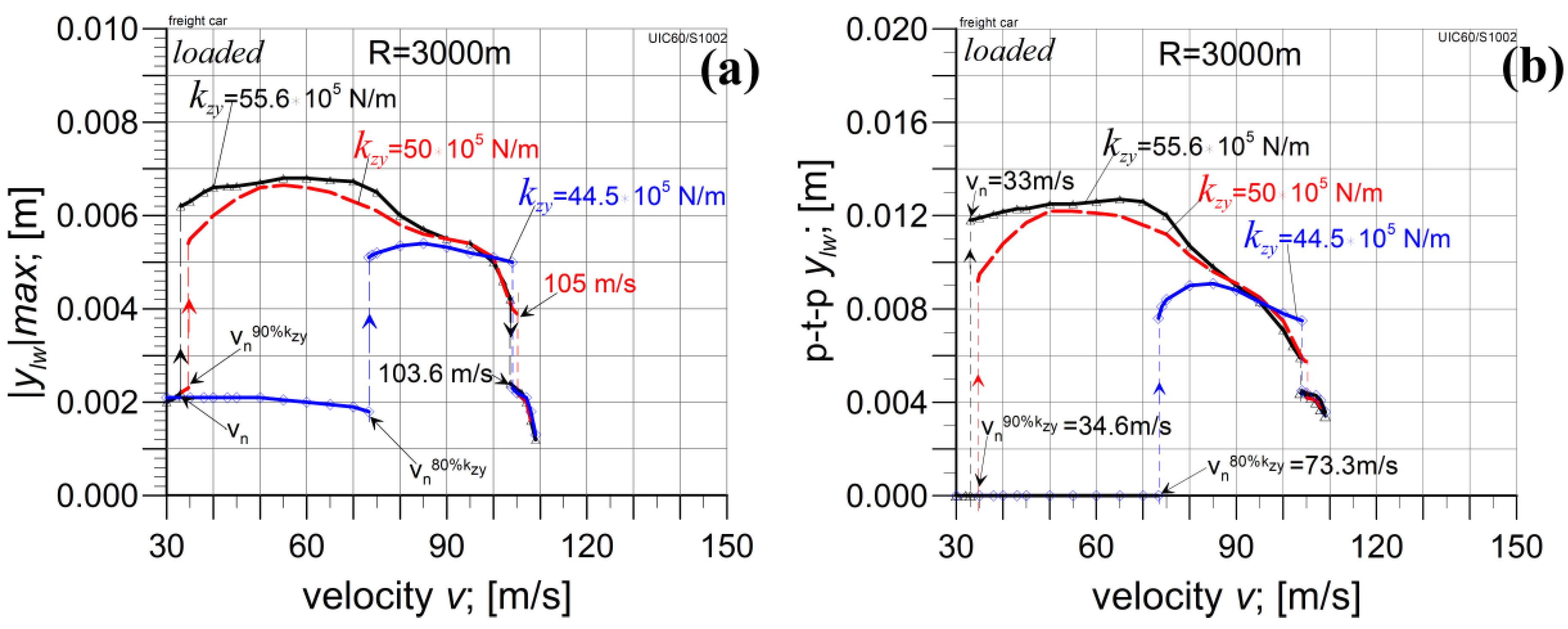
In the case of motion on a CC of R = 3000 m and the nominal value of kzy, the critical velocity vn = 33 m/s (Figure 10). This is slightly lower than the maximum operating (admissible) velocity vad of the studied gondola (vad = 120 km/h ≈ 33.3 m/s). Stable periodic solutions occur up to a velocity v = 103.6 m/s in this case. Then, bifurcation to other periodic solutions appears but with lower values of |ylw|max and p-t-p ylw (approx. p-t-p ylw = 0.004 m). The maximum velocity for which a stable solution exists is v = 109 m/s.
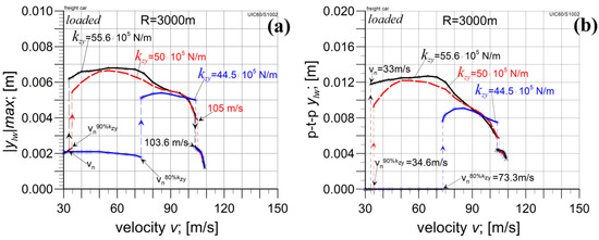
Figure 10.
Influence of lateral stiffness kzy on laden car’s first wheelset. kzy = 55.6 ∗ 105 N/m—nominal value (black line), kzy = 50 ∗ 105 N/m—90% of nominal value (red line), kzy = 44.5 ∗ 105 N/m—80% of nominal value (blue line). Motion on a CC of R = 3000 m: (a) maximum absolute value of lateral; (b) peak-to-peak value of wheelset lateral displacement.
A decrease in the stiffness kzy to 90% of its nominal value (kzy = 50·105 N/m) results in a critical velocity increase up to vn = 34.6 m/s. Periodic solutions last up to v = 105 m/s, and then their bifurcation to other periodic solutions appears but with lower values of |ylw|max and p-t-p ylw (approx. p-t-p ylw = 0.004 m). The maximum value of velocity for which a stable solution exists is v = 108 m/s.
In the next step, the lateral stiffness was reduced to 80% of its nominal value (kzy = 44.5·105 N/m). As a result, there was a dramatic rise in the critical velocity up to vn = 73.3 m/s. Periodic solutions last up to v = 104 m/s, and then their bifurcation to other periodic solutions appears, however, with lower values for |ylw|max and p-t-p ylw. The highest velocity value at which stable solutions existed was v = 109 m/s. Concluding this part of the study, one can state that a reduction in the primary suspension’s lateral stiffness kzy by a dozen percent compared to its nominal value brought about favourable effects on the vehicle motion on the ST and CCs as well. To supplement studies on the influence of kzy on the vehicle model’s solution stability, how reducing kzy affects the tested car model’s properties when it is empty should be checked.
4.3. Empty Car Analysis at Reduced kzy Values
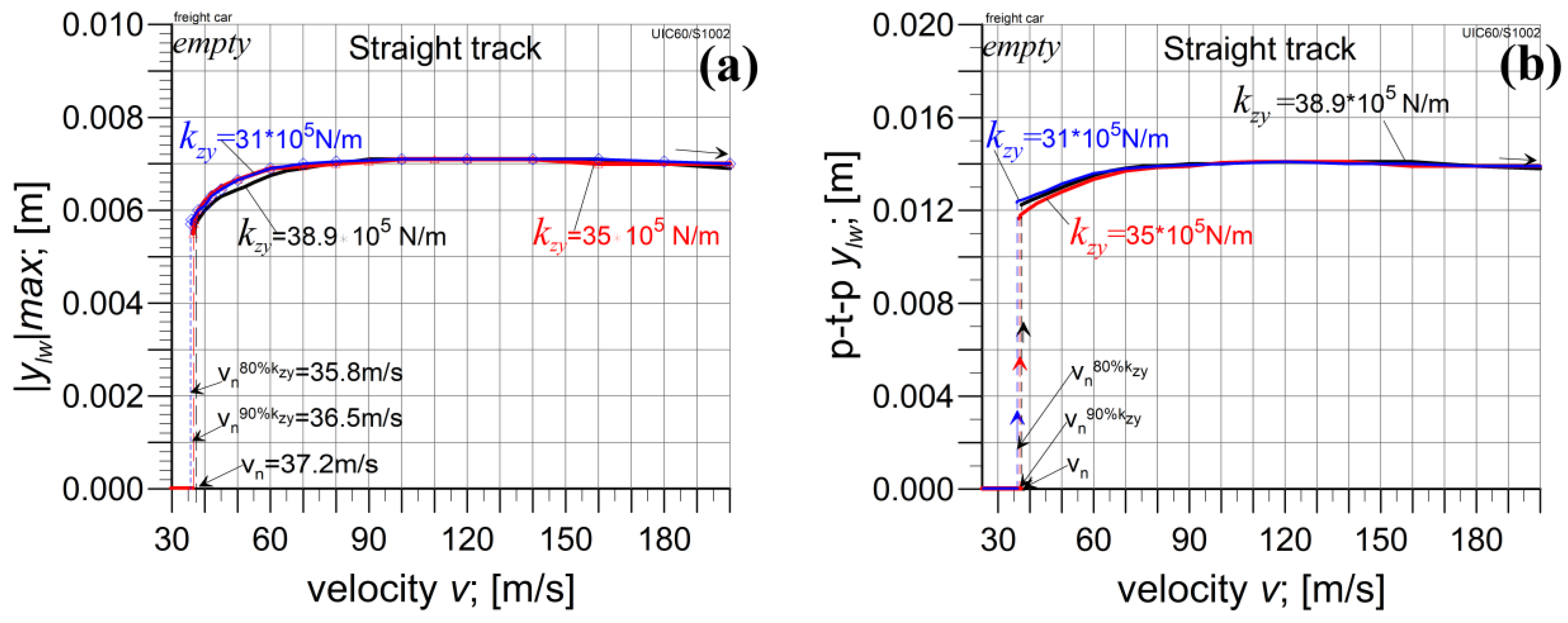
A moderate effect of reducing the lateral stiffness of the primary suspension can be observed on motion along an ST (Figure 11). The critical velocity vn decreases from 37.2 m/s at a nominal kzy value (38.9·105 N/m) to 36.5 m/s for 90% · kzy ≈ 35·105 N/m and to 35.8 m/s for 80% · kzy ≈ 31·105 N/m. So, vn is higher than the required minimum vn = 33.3 m/s. The nature of the model solutions is analogous for each kzy value. So, the solutions are stationary only for velocities v < vn, while for v > vn, periodic solutions appear, which exist up to v > 200 m/s. The solutions’ values are very similar for each value of kzy.
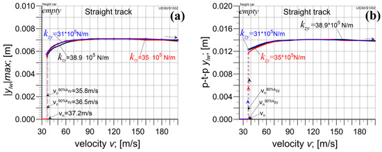
Figure 11.
Influence of lateral stiffness kzy on the empty car’s first wheelset. kzy = 38.9 ∗ 105 N/m—nominal value (black line), kzy = 35 ∗ 105 N/m ≅ 90% of nominal value (red line), kzy = 31 ∗ 105 N/m ≅ 80% of nominal value (blue line). Motion on the ST: (a) maximum absolute value of lateral displacement; (b) peak-to-peak value of wheelset’s lateral displacement.
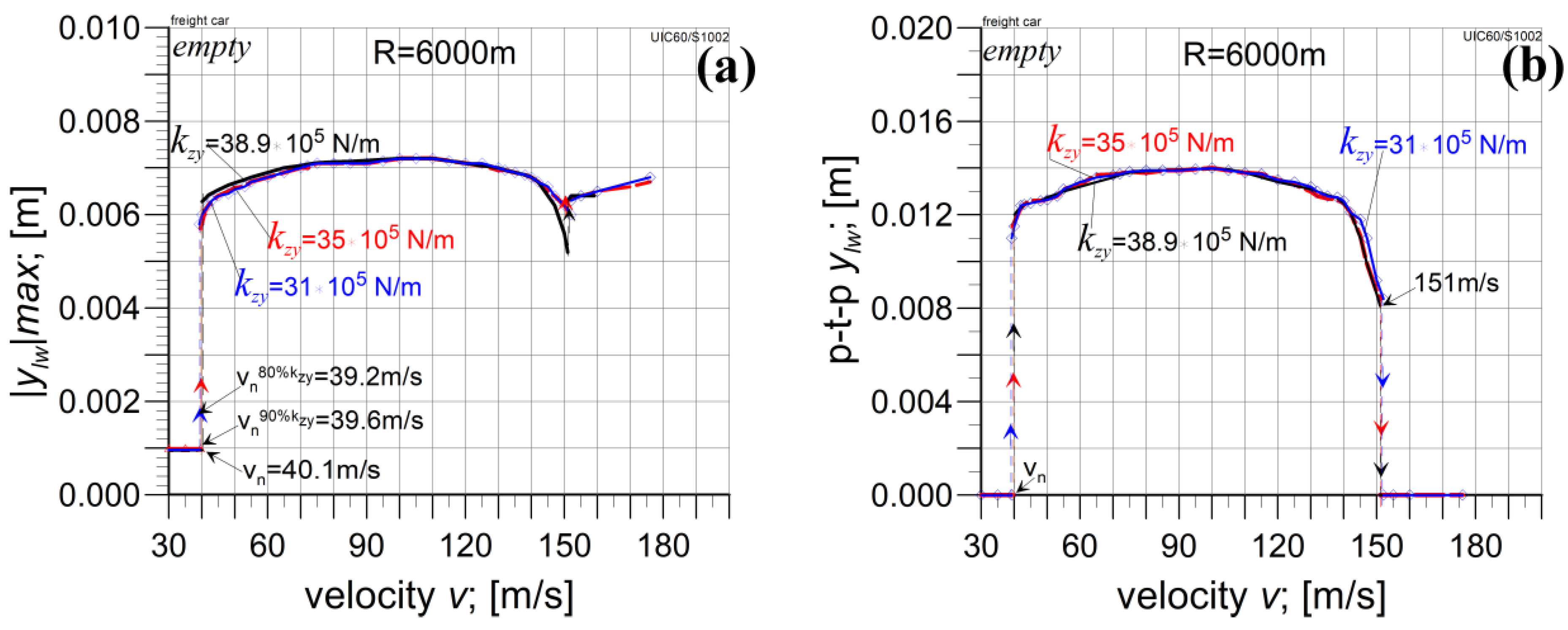
The influence of kzy on the investigated model parameters is also moderate in the case of motion on curved tracks. The critical velocity is 40.1 m/s at the nominal kzy value and with a large R = 6000 m (Figure 12). Reducing the lateral stiffness causes a slight decrease in the critical velocity to the values vn = 39.6 m/s for 90% kzy and vn = 39.2 m/s for 80% kzy, respectively. Stable periodic solutions persist for an increased velocity up to about 151 m/s, followed by bifurcation to stationary solutions. Stable stationary solutions exist up to a velocity of about 176 m/s. The model solution values for the particular kzy values applied are similar in the entire velocity range.
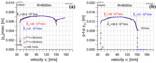
Figure 12.
Influence of lateral stiffness kzy on the empty car’s first wheelset. kzy = 38.9 ∗ 105 N/m—nominal value (black line), kzy = 35 ∗ 105 N/m ≅ 90% of nominal value (red line), kzy = 31 ∗ 105 N/m ≅ 80% of nominal value (blue line). Motion on a CC with R = 6000 m: (a) maximum absolute value of lateral displacement; (b) peak-to-peak value of wheelset’s lateral displacement.
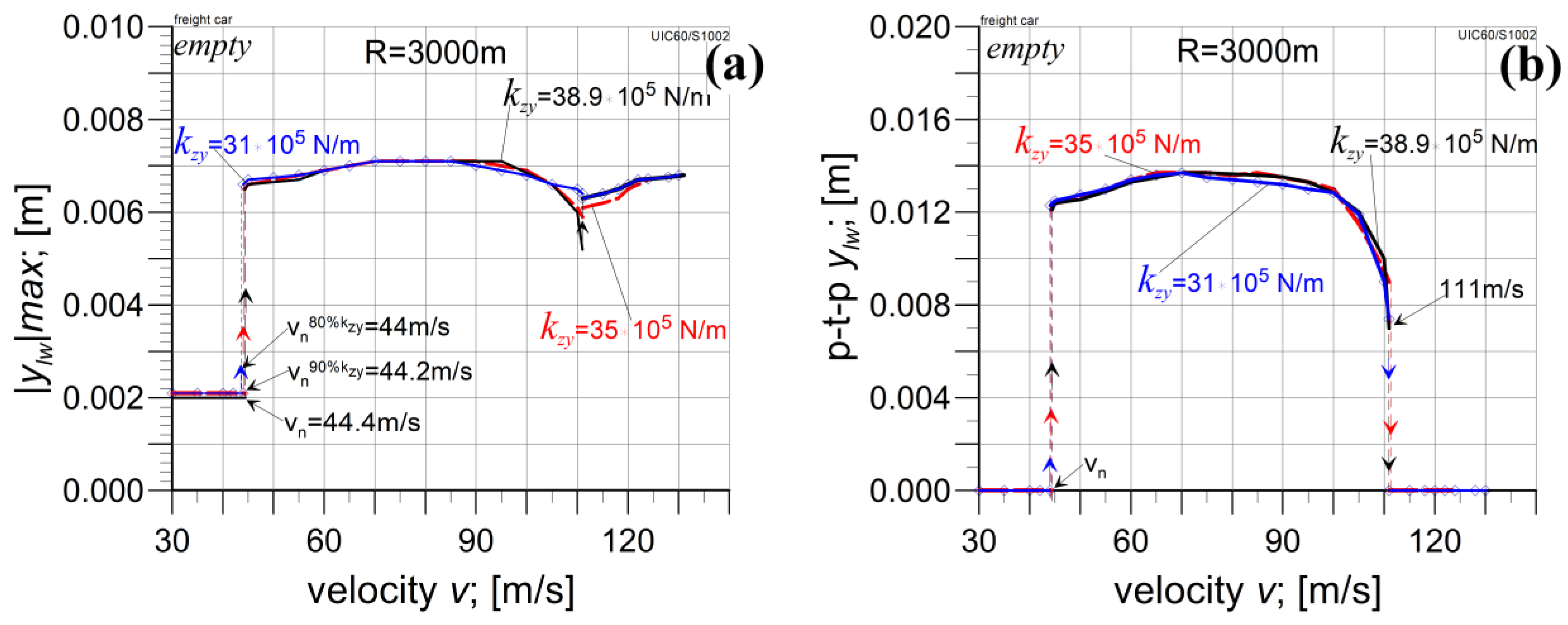
The critical velocity is 44.4 m/s on a CC with a smaller R = 3000 m for the nominal value of kzy = 38.9·105 N/m (Figure 13). Reducing the lateral stiffness kzy to 90% decreased the critical velocity to 44.2 m/s. A further reduction in the lateral stiffness kzy to 80% reduced the critical velocity to 44 m/s only. So, a moderate influence of decreasing kzy on the critical velocity on this route is also observed. The values of the model solutions (|ylw|max and p-t-p ylw) for individual kzy values are similar to the values on the previously studied routes. Thus, it can be observed that reducing kzy to 80% of its nominal value reduces the model’s critical velocity when the car is empty but not more than by 1 m/s.

Figure 13.
Influence of lateral stiffness kzy on the first wheelset of an empty car. kzy = 38.9 ∗ 105 N/m—nominal value (black line), kzy = 35 ∗ 105 N/m ≅ 90% of nominal value (red line), kzy = 31 ∗ 105 N/m ≅ 80% of nominal value (blue line). Motion on a CC with R = 3000 m: (a) maximum absolute value of lateral displacement; (b) peak-to-peak value of wheelset’s lateral displacement.
5. Conclusions
A thorough analysis of the 412W gondola car used in Poland (also by Polish State Railways) in terms of its nonlinear features revealed the existence of several such features. On the other hand, the only unfavourable nonlinear features closely related to the car’s real conditions of exploitation were its stability features. It appeared that unfavourable features of this type concern the studied gondola car in its fully loaded state. The same vehicle in an empty state possesses satisfactory stability properties for the real conditions of its exploitation. The stability map in Figure 5, for the empty car, represents its uniform character for all curve radii R, including on an ST (R = ∞). Most importantly, the nonlinear critical velocities vn for all these R values are above the maximum admissible exploitation velocity vad, equal to 33.3 m/s (120 km/h). The smallest vn = 37.2 m/s exists for an ST. This means that the empty car avoids (is protected against) hunting motion, which is certainly desirable. In the case of the stability map for the fully loaded gondola in Figure 6, the stability features are not as uniform as those of the empty gondola. One can see uniform solutions starting at R = 3000 m and going down to R = 1200 m. On an ST at R = 6000 m, additional, untypical, and, to some extent, unfavourable bifurcations of the solutions from stable periodic solutions to stable stationary solutions exist above the critical velocity vn. Moreover, the vn values for R = ∞, 6000 m, and 3000 m are smaller than or relatively close to the maximum admissible exploitation velocity vad. vn equals 30.8, 45.5, and 33.0 m/s, respectively. So, formally, an ST and R = 3000 m appeared to need correction from the viewpoint of the exploitation velocities. Consequently, the corresponding measures were determined successfully.
The analysis of a gondola freight car with Y25-type bogies shows there is potential to improve its motion properties through minor corrections to the suspension parameter values. From the point of view of the tested vehicle model’s properties, it is possible to increase the car’s critical velocity in the laden state by reducing the lateral stiffness in the primary suspension kzy by a dozen percent or so relative to the nominal value. Reducing kzy to 80% of its nominal value is indicated as a recommendation by the authors. In addition to the higher critical velocity value on an ST (vn = 136.1 m/s), the critical velocities on CCs increased favourably for all R values, too. They were vn = 107.1 and 103.6 m/s for R = 6000 and 3000 m, respectively. Furthermore, a reduction in kzy causes the disappearance of periodic solutions with very small peak-to-peak values on CCs. This could mean an improvement in the quality of real gondola cars of the studied type to negotiate curved tracks. One should notice that reducing kzy to just 90% of its nominal value could also be counted as a successful measure for improving the gondola’s nonlinear features. Then, vn for an ST, at R = 6000 m, and at R = 3000 m equal 36.9, 102.1, and 34.6 m/s, respectively. All of these values are greater than 33.3 m/s. On the other hand, two of them are quite close to vad. In particular, the value for R = 3000 m resulted in a safety margin that was too small. One should also remember here that the accuracy of determining vn is limited.
An essential element of the study’s results, and an important fact at the same time, is that the corrective remedy found for the loaded gondola car does not spoil the results for the empty car. Figure 11, Figure 12 and Figure 13 for the empty vehicle show that for R = ∞, 6000, and 3000 m, decreasing kzy to 90% and 80% of its nominal value changes the critical velocities vn insignificantly. Although such a decrease also decreases vn, which is unfavourable, the changes obtained are negligible. The most significant change in Figure 11 for the ST was the change in vn from 37.2 to 35.8 m/s. It can be seen that 35.8 m/s is still higher enough than vad = 33.3 m/s.
One could treat as certain limitation of the obtained results the calculations having been performed for unworn wheel and rail profiles only. The wear of their profiles can influence a vehicle’s stability properties. We conducted such tests for a two-axle car in [6]. We showed that the critical velocity vn increases slightly when just the wear of the wheels is considered. In the case of worn rails (severe wear was adopted), no matter whether the wheels were worn or not, a drop in vn appeared, which should be regarded as considerable. On the other hand, the wear of wheel and rail profiles concerns all rail vehicles. Thus, eventually, modified cars will be in the same position as the other rail vehicles exploited worldwide.
Finally, it should be noted that the results obtained formally apply only to the particular tested type of car. For other types of freight cars that use Y25 bogies, the observed effects need to be individually studied, and only then can eventual confirmations be made. Note that the gondola studied in the present paper possesses quite different properties in its empty and laden states. This illustrates why the results of this paper could be transferred to another type of car if it had almost identical parameters. On the other hand, the obtained results offer a warning that other cars on Y25 bogies may exhibit unfavourable stability properties, too.
Author Contributions
Conceptualisation, K.Z.; methodology, K.Z. and M.D.; software, K.Z. and M.D.; validation, KZ., M.D., and M.G.-S.; formal analysis, K.Z.; investigation, M.D., M.G.-S., and K.Z.; resources, M.G.-S. and M.D.; data curation, M.D.; writing—original draft preparation, M.D. and K.Z.; writing—review and editing, K.Z.; visualisation, M.D and M.G.-S.; supervision, K.Z.; project administration, K.Z.; funding acquisition, K.Z. and M.G.-S. All authors have read and agreed to the published version of the manuscript.
Funding
This work is a result of the research project financed by the National Center for Research and Development, Poland, under the TANGO program—project no. TANGO-IV-A/0027/2019-00.
Institutional Review Board Statement
Not applicable.
Informed Consent Statement
Not applicable.
Data Availability Statement
The original contributions presented in the study are included in the article, further inquiries can be directed to the corresponding author.
Conflicts of Interest
The authors declare no conflicts of interest.
Appendix A
Table A1.
Parameters of the freight car accepted for research.
Table A1.
Parameters of the freight car accepted for research.
| Notation | Description | Unit | Value | |
|---|---|---|---|---|
| Empty | Loaded | |||
| mcb | Vehicle body mass | kg | 11,000 | 72,000 |
| mb | Bogie frame mass | kg | 1600 | |
| mw | Wheelset mass | kg | 1400 | |
| mab | Axle box mass | kg | 100 | |
| mtb | Bogie’s total mass (mb + 2mw + 4mab) | kg | 4800 | |
| Iξcb | Body’s moment of inertia; longitudinal axis | kg·m2 | 17,300 | 90,055 |
| Iηcb | Body’s moment of inertia; lateral axis | kg·m2 | 188,500 | 1,210,606 |
| Iψcb | Body’s moment of inertia; vertical axis | kg·m2 | 188,140 | 1,231,450 |
| Iξb | Bogie frame’s moment of inertia; longitudinal axis | kg·m2 | 790 | |
| Iηb | Bogie frame’s moment of inertia; lateral axis | kg·m2 | 1000 | |
| Iψb | Bogie frame’s moment of inertia; vertical axis | kg·m2 | 1090 | |
| Iξw | Wheelset’s moment of inertia; longitudinal axis | kg·m2 | 747 | |
| Iηw | Wheelset’s moment of inertia; lateral axis | kg·m2 | 131 | |
| Iψw | Wheelset’s moment of inertia; vertical axis | kg·m2 | 747 | |
| kzz | Vertical stiffness of the primary suspension | kN/m | 1017 | 2280 |
| kzy | Lateral stiffness of the primary suspension | kN/m | 3890 | 5560 |
| kzx | Longitudinal stiffness of the primary suspension | kN/m | 12,000 | 12,000 |
| czz | Vertical damping of the primary suspension | kN·s/m | 7 | 123.3 |
| czy | Lateral damping of the primary suspension | kN·s/m | 42 | 138 |
| czx | Longitudinal damping of the primary suspension | kN·s/m | 100 | |
| k2z | Vertical stiffness of the bogie frame—car body side bearer | kN/m | 22,500 | |
| c2x | Longitudinal damping of the bogie frame—car body side bearer | kN·s/m | 6 | 10 |
| k2ψ | Torsional stiffness between the bogie frame and car body | kN·m/rad | 20 | |
| c2ψ | Torsional damping between the bogie frame and car body | kN·m·s/rad | 0.5 | |
| ap | Half of bogies’ pivot-t-pivot distance | m | 4.5 | |
| a | Semi-wheel base | m | 0.9 | |
| tc | Half the distance between the wheelset’s wheels’ rolling circles | m | 0.75 | |
| hb | Vertical distance between bogie frame centre of mass and track plane | m | 0.69 | |
| hcb | Vertical distance between car body centre of mass and track plane | m | 1.5 | 1.87 |
| rt | Wheel’s rolling radius | m | 0.46 | |
References
- Zboinski, K.; Golofit-Stawinska, M. Dynamics of a Rail Vehicle in Transition Curve above Critical Velocity with Focus on Hunting Motion Considering the Review of History of the Stability Studies. Energies 2024, 17, 967. [Google Scholar] [CrossRef]
- Zboinski, K.; Golofit-Stawinska, M. Investigation into nonlinear phenomena for various railway vehicles in transition curves at velocities close to critical one. Nonlinear Dyn. 2019, 98, 1555–1601. [Google Scholar] [CrossRef]
- Csiba, J. Bogie type anniversary: The bogie type Y25 is over 50 years. In Proceedings of the 10th International Conference on Railway Bogies and Running Gears, Budapest, Hungary, 12–15 September 2016; pp. 253–262. [Google Scholar]
- Pagaimo, J.; Magalheas, H.; Costa, J.N.; Ambrosio, J. Derailment study of railway cargo vehicle using a response surface methodology. Veh. Syst. Dyn. 2022, 60, 309–334. [Google Scholar] [CrossRef]
- Zboiński, K.; Dusza, M. Self-exciting vibrations and Hopf’s bifurcation in non-linear stability analysis of rail vehicles in curved track. Eur. J. Mech. Part A Solids 2010, 29, 190–203. [Google Scholar] [CrossRef]
- Zboiński, K.; Dusza, M. Development of the method and analysis for non-linear lateral stability of railway vehicles in a curved track. Veh. Syst. Dyn. 2006, 44 (Suppl. S1), 147–157. [Google Scholar] [CrossRef]
- Zboiński, K.; Dusza, M. Bifurcation analysis of 4-axle rail vehicle models in a curved track. Nonlinear Dyn. 2017, 89, 863–885, ISSN 0924-090X. [Google Scholar] [CrossRef]
- Bustos, A.; Tomas-Rodriguez, M.; Rubio, H.; Castejon, C. On the nonlinear hunting stability of a high-speed train boogie. Nonlinear Dyn. 2023, 111, 2059–2078. [Google Scholar] [CrossRef]
- Xiao, F.; Hu, J.; Zhu, P.; Deng, C. A method of three-dimensional stability region and ideal roll angle to improve vehicle stability. Nonlinear Dyn. 2023, 111, 2353–2377. [Google Scholar] [CrossRef]
- Sun, J.; Meli, E.; Song, X.; Chi, M.; Jiao, W.; Jiang, Y. A novel measuring system for high-speed railway vehicles hunting monitoring able to predict wheelset motion and wheel/rail contact characteristics. Veh. Syst. Dyn. 2023, 61, 1621–1643. [Google Scholar] [CrossRef]
- Umemoto, J.; Yabuno, H. Parametric and self-excited oscillation produced in railway wheelset due to mass imbalance and large wheel tread angle. Nonlinear Dyn. 2023, 111, 4087–4106. [Google Scholar] [CrossRef]
- Seth, S.; Kudra, G.; Wasilewski, G.; Awrejcewicz, J. Study the bifurcations of a 2DoF mechanical impacting system. Nonlinear Dyn. 2024, 112, 1713–1728. [Google Scholar] [CrossRef]
- Margazoglou, G.; Magri, L. Stability analysis of chaotic systems from data. Nonlinear Dyn. 2023, 111, 8799–8819. [Google Scholar] [CrossRef] [PubMed]
- Guo, J.; Shi, H.; Luo, R.; Zeng, J. Bifurcation analysis of a railway wheelset with nonlinear wheel–rail contact. Nonlinear Dyn. 2021, 104, 989–1005. [Google Scholar] [CrossRef]
- Ge, P.; Wie, X.; Liu, J.; Cao, H. Bifurcation of a modified railway wheelset model with nonlinear equivalent conicity and wheel-rail force. Nonlinear Dyn. 2020, 102, 79–100. [Google Scholar] [CrossRef]
- Yang, C.; Huang, Y.; Li, F. Influence of Curve Geometric Parameters on Dynamic Interactions of Side-Frame Cross-Braced Bogie. In Proceedings ICRT 2021, Second International Conference on Rail Transportation; ASCE Library: Reston, VA, USA, 2022. [Google Scholar]
- Chernysheva, Y.; Gorskiy, A. Methods Proposed for Analysis of Vibrations of Railway Cars. In International Scientific Siberian Transport Forum TransSiberia—2021; TransSiberia 2021; Lecture Notes in Networks and Systems; Manakov, A., Edigarian, A., Eds.; Springer: Cham, Switzerland, 2022; Volume 402. [Google Scholar] [CrossRef]
- Skerman, D.; Colin Cole, C.; Spiryagin, M. Determining the critical speed for hunting of three-piece freight bogies: Practice versus simulation approaches. Veh. Syst. Dyn. 2022, 60, 3314–3335. [Google Scholar] [CrossRef]
- Pandey, M.; Bhattacharya, B. Effect of bolster suspension parameters of three-piece freight bogie on the lateral frame force. Int. J. Rail Transp. 2020, 8, 45–65. [Google Scholar] [CrossRef]
- Sun, J.; Chi, M.; Jin, X.; Liang, S.; Wang, J.; Li, W. Experimental and numerical study on carbody hunting of electric locomotive induced by low wheel-rail contact conicity. Veh. Syst. Dyn. 2021, 59, 203–223. [Google Scholar] [CrossRef]
- Shvets, A.O. Dynamic interaction of a freight car body and a three-piece bogie during axle load increase. Veh. Syst. Dyn. 2022, 60, 3291–3313. [Google Scholar] [CrossRef]
- Guo, J.; Zhang, G.; Shi, H.; Zeng, J. Small amplitude bogie hunting identification method for high-speed trains based on machine learning. Veh. Syst. Dyn. 2023, 62, 1253–1267. [Google Scholar] [CrossRef]
- He, S.; Jonsson, E.; Martins, J.R.R.A. Adjoint-based limit cycle oscillation instability sensitivity and suppression. Nonlinear Dyn. 2023, 111, 3191–3205. [Google Scholar] [CrossRef]
- Wang, X.; Lu, Z.; Wen, J.; Wie, J.; Wang, Z. Kinematics modelling and numerical investigation on the hunting oscillation of wheel-rail nonlinear geometric contact system. Nonlinear Dyn. 2022, 107, 2075–2097. [Google Scholar] [CrossRef]
- Knothe, K.; Böhm, F. History of Stability of Railway and Road Vehicles. Veh. Syst. Dyn. 1999, 31, 283–323. [Google Scholar] [CrossRef]
- Kass-Petersen, C.; True, H. A bifurcation analysis of nonlinear oscillations in railway vehicles. Veh. Syst. Dyn. 1984, 13, 655–665. [Google Scholar]
- True, H. On the theory of nonlinear dynamics and its applications in vehicle systems dynamics. Veh. Syst. Dyn. 1999, 31, 393–421. [Google Scholar] [CrossRef]
- Iwnicki, S. (Ed.) Handbook of Railway Vehicle Dynamics; CRC Press Inc.: Boca Raton, FL, USA, 2006. [Google Scholar]
- Shabana, A.A.; Zaazaa, K.E.; Sugiyama, H. Railroad Vehicle Dynamics: A Computational Approach; Taylor & Francis LLC: Abingdon, UK; CRC: Boca Raton, FL, USA, 2008. [Google Scholar]
- Piotrowski, J.; Pazdzierniak, P.; Adamczewski, T. Curving dynamics of freight wagon with one- and two-dimensional friction damping. In Proceedings of the 10th Mini Conference on Vehicle System Dynamics, Identification and Anomalies, Budapest, Hungary, 6–8 November 2006; Zobory, I., Ed.; pp. 215–222. [Google Scholar]
- Bruni, S.; Vinolas, J.; Berg, M.; Polach, O.; Stichel, S. Modeling of suspension components in a rail vehicle dynamics context. Veh. Syst. Dyn. 2011, 49, 1021–1072. [Google Scholar] [CrossRef]
- Evans, J.; Berg, M. Challenges in simulation of rail vehicle dynamics. Veh. Syst. Dyn. 2009, 47, 1023–1048. [Google Scholar] [CrossRef]
- Chudzikiewicz, A.; Drozdziel, J.; Kisilowski, J.; Zochowski, A. Modelowanie i Analiza Dynamiki Układu Mechanicznego Tor-Pojazd; Państwowe Wydawnictwo Naukowe (PWN): Warszawa, Poland, 1982; ISBN 83-01-04727-5. (In Polish) [Google Scholar]
- Shi, H.; Zeng, J.; Guo, J. Disturbance observer-based sliding mode control of active vertical suspension for high-speed rail vehicles. Veh. Syst. Dyn. 2024. [Google Scholar] [CrossRef]
- Kalker, J.J. A fast algorithm for the simplified theory of rolling contact. Veh. Syst. Dyn. 1982, 11, 1–13. [Google Scholar] [CrossRef]
- Piotrowski, J. Kalker’s algorithm Fastsim solves tangential contact problems with slip-dependent friction and friction anisotropy. Veh. Syst. Dyn. 2010, 48, 869–889. [Google Scholar] [CrossRef]
- Bogusz, W. Technical Stability; PWN: Warszawa, Poland, 1972. (In Polish) [Google Scholar]


Disclaimer/Publisher’s Note: The statements, opinions and data contained in all publications are solely those of the individual author(s) and contributor(s) and not of MDPI and/or the editor(s). MDPI and/or the editor(s) disclaim responsibility for any injury to people or property resulting from any ideas, methods, instructions or products referred to in the content. |
© 2024 by the authors. Licensee MDPI, Basel, Switzerland. This article is an open access article distributed under the terms and conditions of the Creative Commons Attribution (CC BY) license (https://creativecommons.org/licenses/by/4.0/).