Abstract
To tackle the complex challenges inherent in gas turbine fault diagnosis, this study uses powerful machine learning (ML) tools. For this purpose, an advanced Temporal Convolutional Network (TCN)–Autoencoder model was presented to detect anomalies in vibration data. By synergizing TCN capabilities and Multi-Head Attention (MHA) mechanisms, this model introduces a new approach that performs anomaly detection with high accuracy. To train and test the proposed model, a bespoke dataset of CA 202 accelerometers installed in the Kirkuk power plant was used. The proposed model not only outperforms traditional GRU–Autoencoder, LSTM–Autoencoder, and VAE models in terms of anomaly detection accuracy, but also shows the Mean Squared Error (MSE = 1.447), Root Mean Squared Error (RMSE = 1.193), and Mean Absolute Error (MAE = 0.712). These results confirm the effectiveness of the TCN–Autoencoder model in increasing predictive maintenance and operational efficiency in power plants.
1. Introduction
Gas turbines, which play an essential role in modern power generation, have several advantages that make them essential to meet global energy demands. First of all, their high efficiency, especially in combined cycle configurations, ensures optimal energy use [1]. This efficiency is coupled with a fast start-up capability, a critical feature that allows them to respond quickly to fluctuations in electricity demand, making them invaluable in complementing intermittent renewable energy sources, such as wind and solar. While they are primarily fueled by natural gas, their versatility allows them to operate with a variety of fuels and ensures flexibility in resources. This flexibility is highlighted by the compact size of gas turbines, enabling them to be strategically located close to points of consumption and minimizing transmission losses. Moreover, natural gas combustion results in lower CO2 emissions than coal, which is in line with global efforts to combat climate change [2].
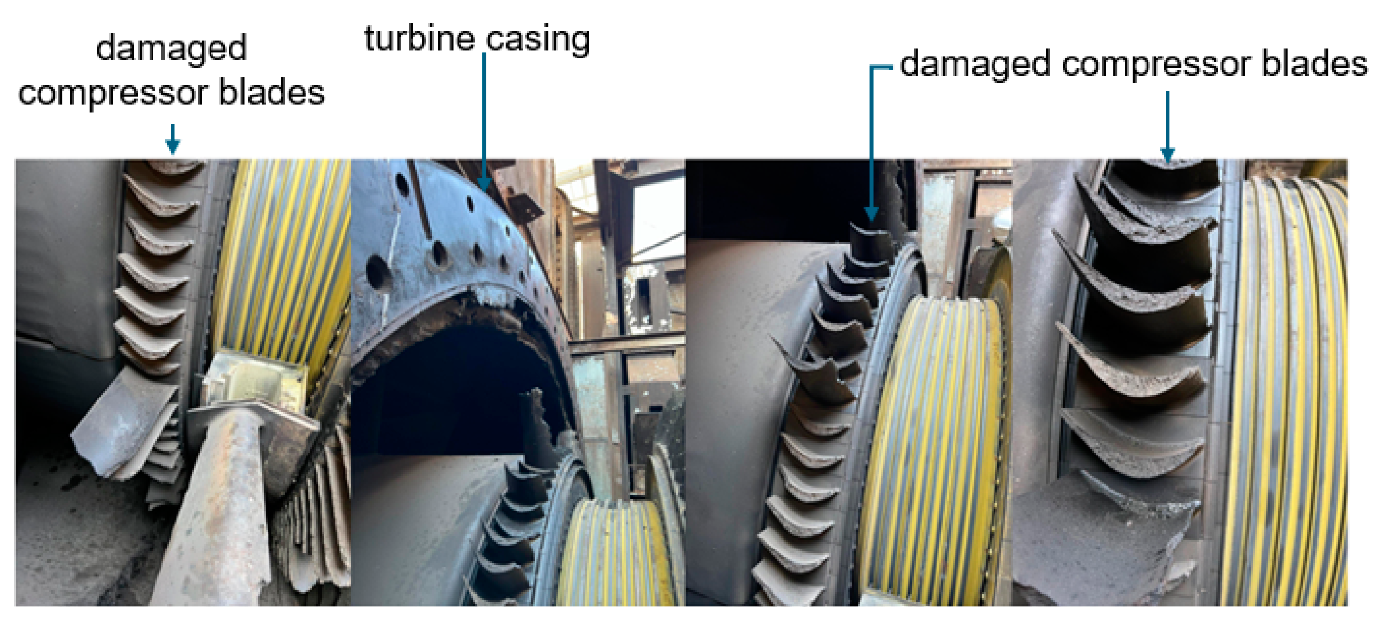
The cogeneration potential of gas turbines further emphasizes their efficiency, as they can simultaneously meet electricity and heating needs [3]. Technological advances continue to refine their performance, making them more environmentally friendly and operationally flexible. Economically, they require a shorter time to build and incur lower capital costs compared to some traditional power sources, ensuring cost-effective power generation. In the evolving energy landscape, with increasing emphasis on decentralization and environmental information, gas turbines remain central, and bridge the gap between conventional and renewable energy sources [4]. However, even with these undeniable advantages, gas turbines are not without their challenges. One of the main issues is that the compressors can become fouled due to particle accumulation, which leads to reduced performance [5]. In certain scenarios, airflow may reverse and compromise system integrity. During combustion, a critical phase wherein the fuel is ignited to produce energy, anomalies such as flameout or flashback may occur, compromising the safety of the system [6]. Turbine blades, exposed to harsh operating conditions, may experience erosion, Foreign Object Damage (FOD), or catastrophic failures [7,8,9]. Figure 1 shows the damaged turbine of the Kirkuk gas power plant.

Figure 1.
A damaged turbine in the Kirkuk gas power plant located in Iraq.
Bearings, which are essential to facilitate seamless motion, can overheat and seals may fail [10]. In addition, the lubrication system, which plays a key role in reducing wear, is vulnerable to contamination or insufficient oil circulation [11]. Also, the cooling mechanism responsible for maintaining the optimal operating temperature may encounter obstructions that lead to undesirable overheating. If the sensors send incorrect data, the control systems as well as the operations management link are disrupted. The fuel system is also not exempt from challenges. For example, issues such as clogged nozzles and poor fuel quality can prevent efficient combustion [12]. Structural integrity is another concern. In this regard, small-scale (i.e., nano and micro) cracks appear and grow in the structure due to repeated thermal cycling. Furthermore, vibrational disturbances may occur, potentially destabilizing the system. Electrical components, including generators, are also prone to failure. Failures in gas turbine power plants can lead to significant operational and economic consequences. Emergency incidents often involve operational downtime that causes potential power outages or reliance on alternate power sources. Even without a complete shutdown, efficiency is reduced, resulting in increased fuel consumption and higher operating costs. Such errors also increase maintenance costs due to necessary repairs or replacement of components. From a safety perspective, certain failures can create hazards such as fire or explosion and endanger facility personnel. Environmentally, the increase in greenhouse gas emissions due to incomplete combustion can have adverse effects. These operational challenges can also damage an electricity provider’s reputation, lead to contractual penalties, and compromise the reliability of the wider electricity grid. Therefore, the regular maintenance and monitoring of gas turbines is very important to reduce these challenges [13]. A variety of sensors and techniques are used to detect and prevent problems (e.g., faults) in gas turbines. One of the main methods is vibration analysis, in which piezoelectric accelerometers play a key role [14]. These sensors measure vibration abnormalities that, if left unchecked, can lead to potential imbalance or bearing failures. Complementing this inspection is thermography, where tools such as infrared thermometers and advanced thermal cameras map out temperature profiles [15]. Their ability to detect even small thermal deviations can highlight operational inefficiencies, wear, or potential component failures. Additionally, the different world of acoustic emissions is driven by the use of specialized piezoelectric sensors or high-quality microphones [16]. These devices, attuned to high-frequency sound waves, are essential for proactively detecting internal cracks or leaks. Oil analysis, critical to maintenance, uses spectrometry to identify unwanted metal contaminants. Moreover, digital viscometers and ferrography provide accurate assessments of lubricant quality, signaling potential wear and degradation [17]. Performance monitoring uses various sensors such as pressure transducers, flow meters, and thermocouples to provide instant data [18]. This helps to quickly detect any deviation from normal performance standards. In the case of Non-Destructive Testing (NDT) [19], the X-ray machine is restrained to identify defects in such a way that the integrity of the equipment is maintained. Modern control systems, supported by platforms such as SCADA and PLC, seamlessly integrate with countless sensors and provide a comprehensive diagnostic view. This technological advantage is enhanced by data analytics and machine learning. With countless sensors continuously sending data to cloud systems, advanced AI algorithms analyze this vast information and predict wear trends and possible component failures [20]. In addition, precision instruments such as digital pressure gauges and ultrasonic flowmeters increase our understanding of system health and highlight any irregularities. The proposed sensors can provide immediate insights into the operational status of a system. However, machine learning can perform a more comprehensive analysis of this collective information and identify patterns or anomalies that can be a sign of impending faults [20]. This method enables a more proactive approach to maintaining system integrity and predicting and preventing potential failures before they occur. For instance, a study titled “On accurate and reliable anomaly detection for gas turbine combustors: A deep learning approach” emphasizes the application of deep learning for anomaly detection in gas turbine combustions and emphasizes the accuracy of unsupervised learning models [21]. Another significant contribution is the introduction of a novel fault detection method for gas turbines using transfer learning with Convolutional Neural Networks (CNNs), as detailed in “A novel gas turbine fault diagnosis method based on transfer learning with CNN”. This method highlights the superiority of CNNs over other Deep Neural Networks (DNNs) in gas turbine fault diagnosis [22]. Furthermore, the research on “Fault diagnosis of gas turbine based on partly interpretable convolutional neural networks” addresses the importance of model interpretability and shows that partially interpretable CNNs can play a role in fault diagnosis [23]. In addition to the above, many studies have been conducted in this field, and it is not possible to include all of them in this article. However, Failure Mode and Effects Analysis (FMEA) can also be effectively used in this field [24]. In this regard, Tang et al. presented a new FMEA technique based on the improved pignistic probability transformation function and grey relational projection method [25]. This approximation was presented for use in aircraft turbine rotor blades and the steel manufacturing process.
The primary contributions of this paper include the exploration and description of machine learning and deep learning techniques specifically designed for fault detection in gas turbine power plants. Using our custom dataset, we have developed a TCN–Autoencoder model for anomaly detection. Furthermore, we have compared our model with other models such as the Gated Recurrent Unit (GRU)–Autoencoder, Long Short-Term Memory (LSTM)–Autoencoder, and Variational Autoencoder (VAE). Through this evaluation, we aim to identify an accurate technique and provide valuable insight for future research and practical applications in the field of gas turbine fault detection and prediction.
2. Literature Review
Traditional methods for fault diagnosis in gas turbines, such as physics-based models and rule-based expert systems [26], have played a fundamental role in our understanding and diagnosis of faults in these critical machines. These approaches are respected for their accuracy in identifying and characterizing faults, providing a robust framework for fault analysis. However, they have inherent limitations when applied to real-time scenarios, mainly due to their computational requirements and difficulty in adapting to emerging or unconventional fault patterns [27]. Another class of methods, signal processing techniques, has been widely used in the analysis of sensor data from gas turbines. Techniques such as Fourier analysis and wavelet transform [28] have shown their effectiveness in detecting anomalies in data. However, these methods often struggle with the challenge of distinguishing benign operational changes from actual faults when operating in real-time scenarios. In the following, the details of different algorithms for gas turbine fault diagnosis are discussed in Table 1.

Table 1.
Advantages and disadvantages of different algorithms/methods applied for fault detection in gas turbines.
In recent years, there has been a significant shift towards the adoption of machine learning (ML) algorithms, especially deep learning models, for real-time fault diagnosis in gas turbines. This transition is driven by the potential of these advanced techniques to significantly increase fault detection accuracy and adaptability. Models such as Recurrent Neural Networks (RNNs), Autoencoders, Convolutional Neural Networks (CNNs), and Temporal Convolutional Networks (TCNs) have emerged as powerful tools for time-series data analysis in various applications. Real-time anomaly detection in time-series data is a multifaceted challenge, and choosing the most appropriate deep learning method depends on specific characteristics of the data and unique application requirements. TCNs have been highlighted for their ability to process sequences in parallel, dissimilar to RNNs that work in a stepwise manner, making them particularly efficient for real-time scenarios. Furthermore, their architecture, which uses dilated convolutions, enables them to capture long-range dependencies in the data, which is a critical factor for accurate anomaly detection in time-series data. Choosing the best method for fault detection in gas turbines depends on various factors, including data complexity, availability of labeled anomaly data, desired trade-offs between false positives and false negatives, and computational resources. Considering the advantages offered by TCNs, they present a compelling case for real-time fault diagnosis in gas turbines, especially when the balance between computational efficiency and diagnosis accuracy is considered.
3. Data Collection
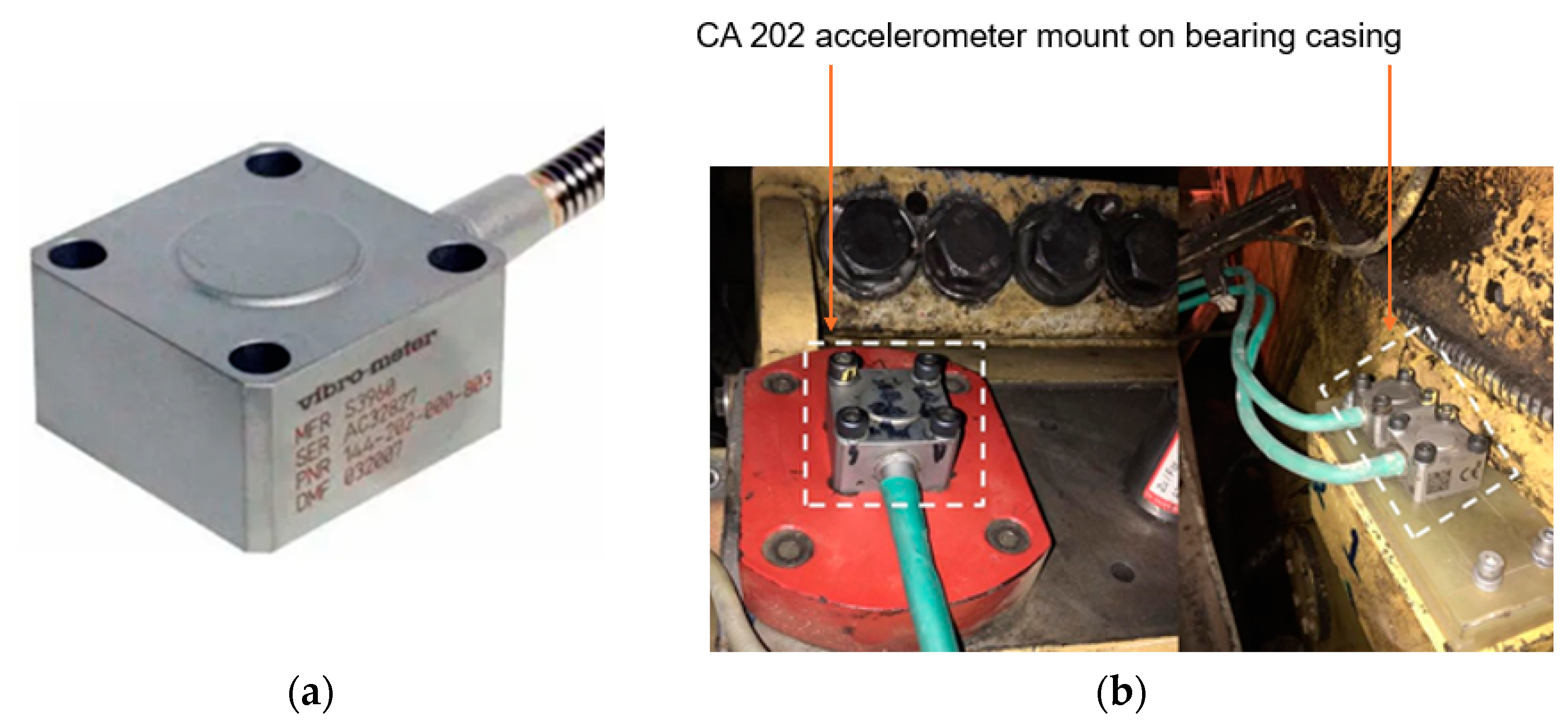
The present study uses a comprehensive dataset derived from the Kirkuk gas power plant, which is currently being upgraded to a Combined Cycle Power Plant (CCPP). Data collection spanned the entire month of December 2021, starting at 12:00 a.m. on the 1st and ending at 11:59 p.m. on the 31st. The dataset includes the output of four CA 202 accelerometers installed on four bearings (Figure 2a) [34]. These readings show plant operations at any given time, including machine activity, load levels, and signs of wear.
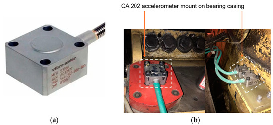
Figure 2.
Equipment used to monitor turbine vibrations in Kirkuk gas power plant, Iraq, including (a) CA 202 accelerometer and (b) accelerometer installation [34].
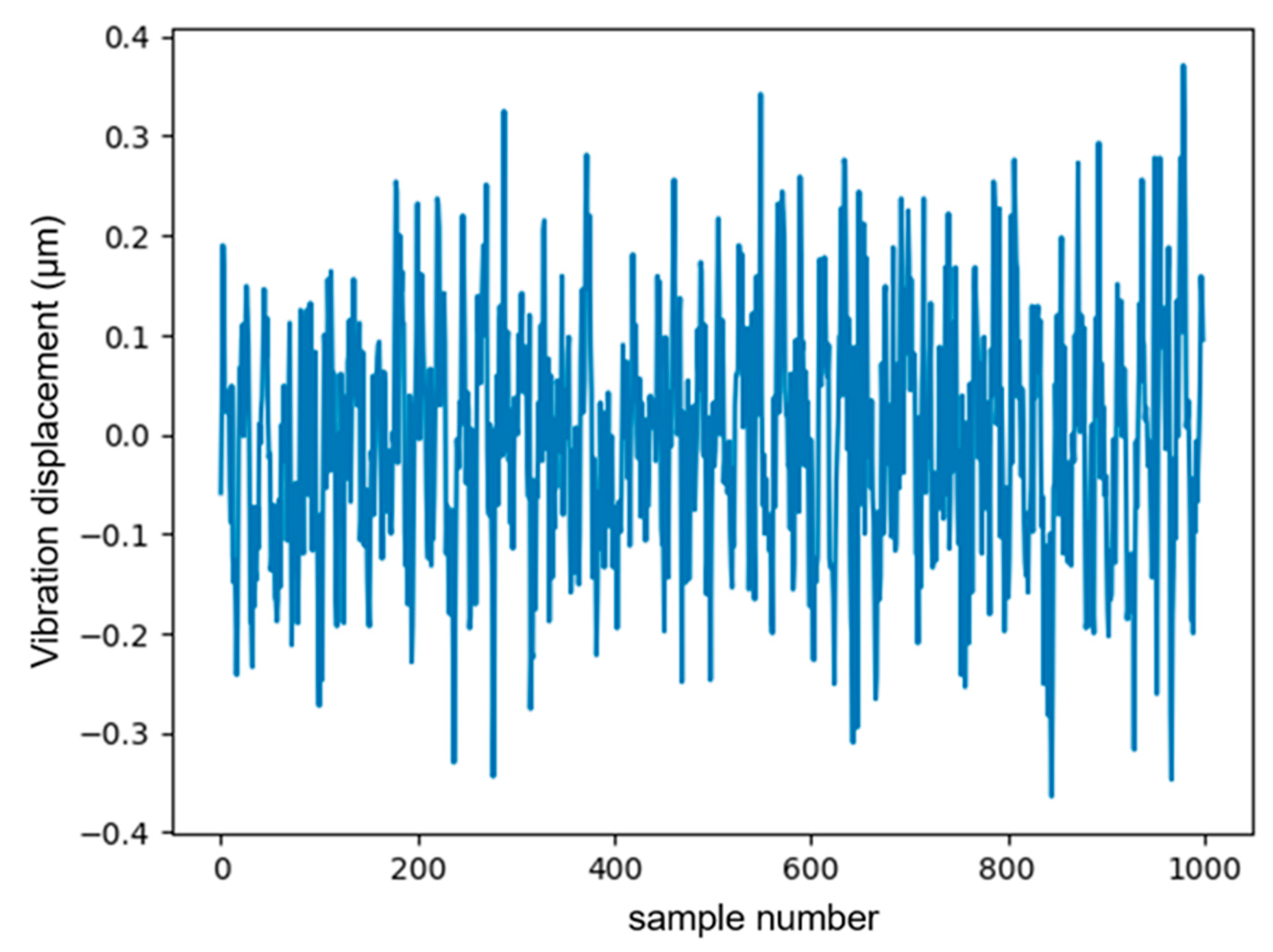
The CA 202 accelerometer has internal body insulation with a symmetrical polycrystalline shear-mode measuring element. This piezoelectric accelerometer has a sensitivity rate of 100 pC/g at 120 Hz. This device is resilient and can withstand transient overloads with a maximum weight of 250 g. With its linear fine-tuning, it maintains 1% accuracy from 0.0001 g to 20 g with an average deviation of up to 2% between the peak range of 20 g and 200 g. Its dynamic measurement range is from a tiny 0.0001 g to a remarkable peak of 200 g. When discussing its features, this accelerometer exhibits a transverse sensitivity of 5% and resonates at a nominal frequency of 11 kHz. The frequency response is consistent within 5% from 0.5 Hz to 3000 Hz, with a low threshold determined by the associated conditioner, and exhibits a 10% response rate between 3 kHz and 4.5 kHz. Amplifying the accelerometer capabilities is the IPC 704 signal regulator. This device effectively converts the piezoelectric transducer signal into current or voltage. In this regard, standard 2- or 3-wire cables can carry this signal without the need for expensive connectors. In addition, it exhibits admirable temperature stability, typically recorded at 100 ppm/°C [35]. Figure 3 presents an example of the collected data.

Figure 3.
An example of data collected from the VIBRO-METER monitoring system installed in the Kirkuk gas power plant.
As mentioned earlier, the data were collected using accelerometers installed on key bearings of the gas turbine in the Kirkuk gas power plant (Figure 2). For this purpose, each sensor was calibrated with a vibration sampling rate of 1 kHz. The reason for using data capturing with such a resolution (high level) was to ensure the accuracy necessary to detect even subtle anomalies in turbine operation. The turbines were monitored in different operational modes, including start-up, normal operation, and shutdown phases. This diversity ensures that our model is robust to different states of turbine operating. Temperature, pressure, and humidity levels were monitored continuously, as these can significantly affect the sensor reading. A total of about 1,000,000 individual data points were collected over a one-month period, which is generally remarkable data for training and testing a robust model. Data were sampled every second, and each sample included multi-dimensional readings from each accelerometer.
Data Pre-Processing
The success of an anomaly detection model depends significantly on the quality of the input data. This study performed a series of data pre-processing steps to ensure that the data are both representative of real patterns and prepared for effective model training. This operation is described below:
Noise Reduction (NR): In this study, a Moving Average Filter (MVF) was used to reduce noise [36]. This method refines the dataset by averaging a predefined number of consecutive data points in a specified window, effectively smoothing out short-term fluctuations and increasing the clarity of underlying patterns. By filtering out unwanted noise, we ensure that the data fed into our deep learning model represent actual plant operating patterns, increasing the accuracy and reliability of any resulting insight or diagnosis. Figure 4 displays an output from applying an MVF on the member of the collected dataset. The MVF window size of 10 was considered.
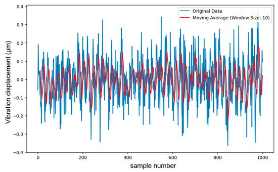
Figure 4.
The result of applying an MVF on the collected data.
Handling Missing Data (HMD): Maintaining the seamless flow and validity of this time-series dataset is critical, as any disruptions or gaps can potentially distort its inherent temporal sequences. For this purpose, we chose the linear interpolation technique to adeptly tackle and rectify such inconsistencies. This method estimates missing values based on adjacent data points and maintains the dataset’s flow. Especially for time-sensitive readings such as vibrations, linear interpolation assumes a constant change between consecutive data points and provides a smooth transition for missing values. However, it is important to consider the root cause of any data omissions. If they are caused by specific events, such as equipment failure, more specific treatment may be required. After imputation, the dataset was checked to ensure that the introduced values did not distort the true patterns.
Anomalies were initially labeled based on historical maintenance records and confirmed by experienced engineers at the plant. The dataset was divided into 80% for training and 20% for testing, which ensures sufficient data for learning and also reserves an unbiased subset for evaluation each time.
4. TCN–Autoencoder
The proposed model presented in the current study introduces a new approach for accurate anomaly detection by taking advantage of the synergistic capabilities of Temporal Convolutional Network (TCN) and Multi-Head Attention (MHA) mechanisms. This model has a major challenge that requires models that are able to recognize intricate temporal patterns and subtle deviations that act as anomaly indicators. This architecture is designed to capture a wide range of temporal dependencies in time-series data and increase model sensitivity to anomalies.
Current methods for fault diagnosis in gas turbines, which mainly focus on traditional machine-learning techniques and rule-based systems, face several important challenges:
- (1)
- Limited adaptability: many existing models, including rule-based systems and early machine learning, try to adapt to the variable operating modes of modern gas turbines; this limits their effectiveness in dynamic environments where operational parameters change frequently.
- (2)
- Scalability issues: traditional methods often do not scale well with the increasing volume of data generated by modern sensor technologies installed in turbines, leading to performance degradation as the volume of data increases.
- (3)
- Insensitivity to subtle anomalies: most legacy systems are designed to detect large-scale deviations, which makes them less efficient at detecting subtle anomalies that can precede major faults.
- (4)
- High false alarm rate: due to their generalized nature, these systems often have a high rate of false alarms, which can lead to unnecessary shutdown and maintenance activities, and increase operating costs.
Meanwhile, our proposed model introduces several innovative features that address the above-mentioned challenges:
- (A)
- TCN architecture: Unlike traditional RNNs, TCNs offer efficient processing through parallelization and can capture long-range dependencies in time-series data. This makes our model highly effective in real-time fault detection scenarios.
- (B)
- MHA mechanism: This feature allows the model to focus on different parts of the data simultaneously, enhancing its ability to detect subtle anomalies that are indicative of potential faults. This directly addresses the issue of insensitivity in many traditional models.
- (C)
- Anomaly detection through reconstruction: The autoencoder aspect of the model focuses on reconstructing the input data and identifying deviations from the norm. This approach reduces false positives by distinguishing between normal fluctuations and actual anomalies.
- (D)
- Scalability and adaptability: Our model is designed to be scalable by incorporating additional sensor data and adapting to new unforeseen operational conditions without requiring extensive retraining.
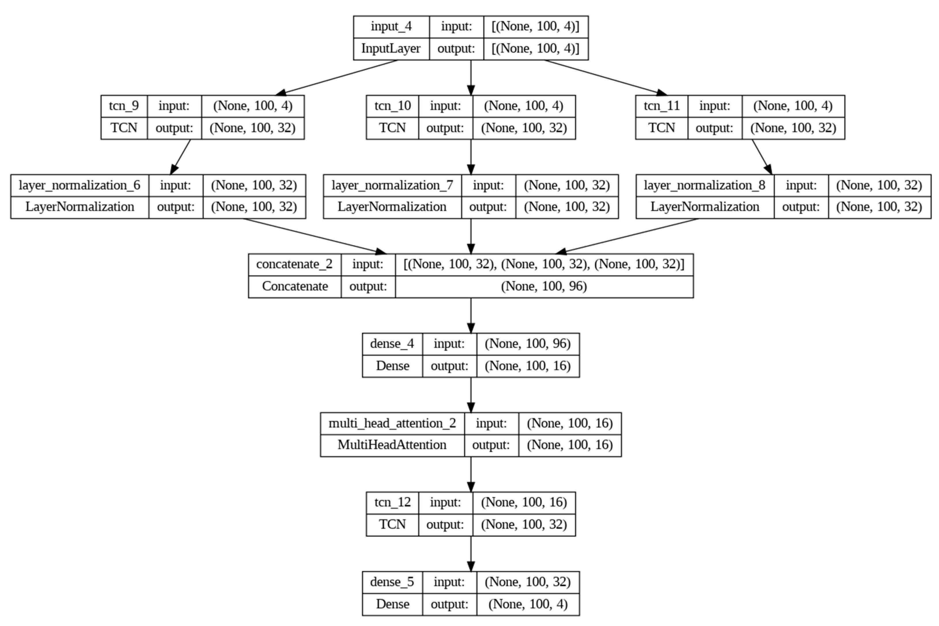
By incorporating these features, our TCN–Autoencoder model not only outperforms traditional fault detection systems in terms of accuracy and efficiency but also significantly enhances predictive maintenance capabilities. This novel approach is expected to reduce maintenance costs and improve the reliability and safety of gas turbine operations. Figure 5 presents the structure of the advanced multi-scale TCN–Autoencoder. The core of the model is built on TCN blocks, which are suitable for sequential data due to their convolutional nature. Unlike traditional convolutional networks, TCNs offer the advantage of larger receptive fields through expanded convolutions, making them ideal for time-series data where long-term dependencies are critical. In this model, several TCN branches were developed in parallel, each with a unique dilation rate (dilation_rate parameter with values of 1, 2, and 4) which helps the network capture different levels of detail in time-related features. This multi-branch setup ensures that the model can detect anomalies on different time scales, from instantaneous to longer deviations. Following the TCN layers in each branch, it applies layer normalization to normalize activations and stabilize the learning process. This is especially important in deep networks, where the scale of activation can vary significantly, potentially leading to unstable gradients and hindering convergence. Algorithm 1 presents the pseudocode of the multi-scale TCN–Autoencoder designed for this study.
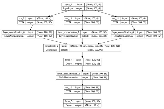
Figure 5.
The multi-scale TCN–Autoencoder architecture with layer normalization designed in this study.
The innovation of our model lies in the integration of an MHA mechanism in the bottleneck layer. After the TCN branches have merged their outputs, a dense layer condenses the feature set, which is then processed by the Multi-Head Attention (Algorithm 1). This mechanism allows the model to simultaneously focus on different segments of the time series and capture intricate interdependencies that a single attention head might miss. It is this ability to weigh various parts of the sequence differently that enables the model to detect anomalies that might only become apparent by considering the broader context of the data. A model decoder designed to mirror the encoder’s multi-scale TCN architecture reconstructs the input data from a compressed representation of the bottleneck. The goal here is not just to replicate the input, but to do so in a way that highlights discrepancies that indicate anomalies. It is through this reconstruction error that the model reveals potential anomalies with larger errors indicating significant deviation from the norm. To ensure robust training and evaluation, the model is compiled using the Adam optimizer (Adam), with the Mean Squared Error [37] as the primary loss function (loss = ‘mean_squared_error’) (Algorithm 1). This choice represents the reconstruction-centric nature of our approach, where the fidelity of the reconstructed signal to the original signal is very important.
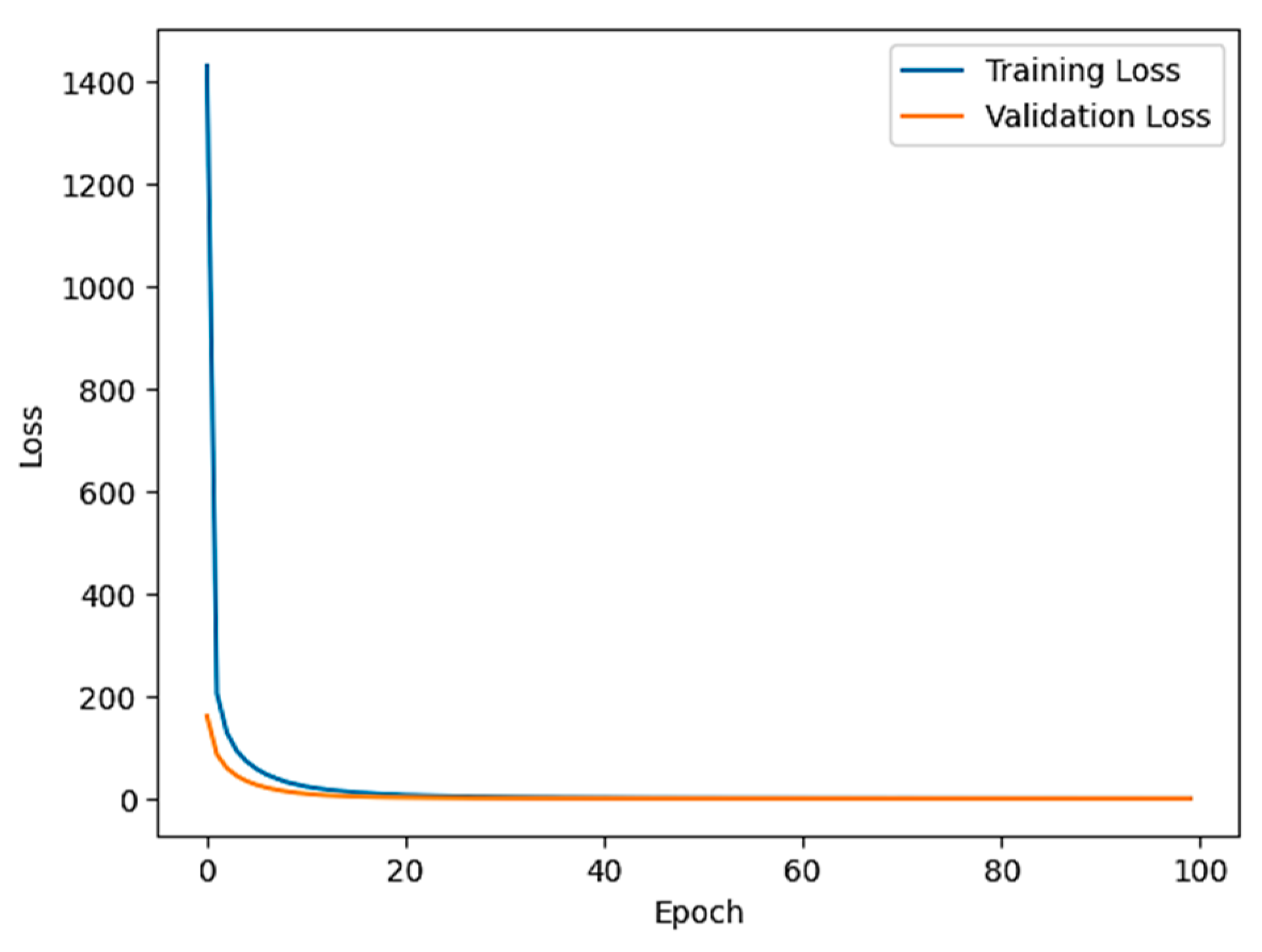
Figure 6 illustrates the loss function of the training and validation loss curves of the anomaly detection model over 100 epochs. Both losses decrease sharply in the early epochs, indicating rapid learning, and then plateau, indicating convergence. The closeness of the training and validation loss indicates that the model generalizes well without overfitting. Moreover, the architecture of the multi-scale TCN-Autoencoder model is summarized in Table 2.
| Algorithm 1 Anomaly Detection Model with TCN and Multi-Head Attention |
| 1: Input: Time-series data X with shape (T, F) where T is the number of time steps and F is the number of features. 2: Output: Reconstructed time-series , Anomaly scores 3: procedure TCNBRANCH(X, dilation_rate) 4: Apply TCN layer with specified dilation_rate 5: Apply LayerNormalization 6: return TCN output 7: end procedure 8: procedure ENCODER(X) 9: for rate in [1, 2, 4, 8] do 10: TCN_output[rate] ← TCNBRANCH(X, rate) 11: end for 12: Encoded ← Concatenate(TCN_output[1], TCN_output[2], TCN_output[4]) 13: return Encoded 14: end procedure 15: procedure BOTTLENECK(Encoded) 16: Bottleneck ← Dense layer on Encoded 17: AttentionOutput ← MultiHeadAttention(Bottleneck, Bottleneck) 18: return AttentionOutput 19: end procedure 20: procedure DECODER(AttentionOutput) 21: Apply TCN with dilation rates [1, 2, 4] 22: Decoded ← LayerNormalization 23: return Decoded 24: end procedure 25: procedure ANOMALYDETECTIONMODEL(X) 26: Encoded ← ENCODER(X) 27: AttentionOutput ← BOTTLENECK(Encoded) 28: Decoded ← DECODER(AttentionOutput) 29: , ← Dense layer on Decoded to reconstruct input shape 30: return , ComputeAnomalyScores(X, ) 31: end procedure 32: ReconstructedX, AnomalyScores ← ANOMALYDETECTIONMODEL(X) |

Figure 6.
Loss curves for the anomaly detection model, showing a rapid decrease and subsequent stabilization in both training and validation loss over 100 epochs.
Table 2.
Summary of architecture of multi-scale TCN–Autoencoder model.
5. Results and Discussion
Our research includes a comprehensive comparative analysis of the TCN–Autoencoder model with other established methods in the field of time-series anomaly detection. For a robust comparison, we selected a set of models known for their performance in this field, including the GRU–Autoencoder, LSTM–Autoencoder, and Variational Autoencoder (VAE). First, we explain the details of these well-known models. Then, we engage in a discussion that compares the performance of these models with the TCN–Autoencoder model, aiming to highlight the performance of our model in detecting anomalies in time-series data.
5.1. A Brief Description of the Models Used for Comparison
- GRU–Autoencoder: This model is built around the Gated Recurrent Unit (GRU), a type of RNN that is suitable for capturing sequential patterns while avoiding some of the gradient vanishing issues associated with traditional RNNs. Algorithm 2 starts by defining the input shape, which provides flexibility in handling sequences of different lengths and dimensions. The ‘inputs’ variable is initialized as the input layer and holds the data in the specified shape. The core of the model consists of an encoder–decoder architecture. In the encoding phase, the input sequence is processed by a GRU layer with 64 units. This GRU layer effectively compresses the input data into a fixed-size latent representation that is stored in the ‘encoded’ variable. The ‘return_sequences’ parameter is set to ‘False’, which means it will only record the final hidden state of the GRU and summarize the input sequence. The decoding phase starts with a ‘RepeatVector’ layer, which repeats the latent representation to match the length of the original input sequence. Another GRU layer is then used to decode the repeated representation, effectively reconstructing the input sequence. By setting ‘return_sequences’ to ‘True’, this GRU layer generates an output sequence that closely resembles the original input sequence. The last step involves using the ‘TimeDistributed’ layer along with a ‘Dense’ operation. This combination allows each time step in the output sequence to be reconstructed independently, effectively mapping the latent representation to the original data space. The reconstructed sequence is stored in the ‘decoded’ variable.
| Algorithm 2 Pseudocode for building a GRU-Autoencoder |
| 1: function BUILD_GRU_AUTOENCODER(input_shape) 2: inputs ← Input(shape=input_shape) 3: encoded ← GRU(64, return_sequences=False)(inputs) 4: decoded ← RepeatVector(input_shape[0])(encoded) 5: decoded ← GRU(64, return_sequences=True)(decoded) 6: denseLayer ← Dense(input_shape[−1]) 7: decoded ← TimeDistributed(denseLayer)(decoded) 8: autoencoder ← Model(inputs, decoded) 9: autoencoder.compile(optimizer=Adam(learning_rate=0.001), loss=’mean_squared_error’) 10: return autoencoder 11: end function |
- LSTM–Autoencoder: This model is a neural network architecture commonly used for sequencing tasks. The model uses Long Short-Term Memory (LSTM) cells, a type of recurrent neural network (RNN) that efficiently captures temporal dependencies in sequential data while mitigating the vanishing gradient problem. Algorithm 3 starts by specifying the input shape and provides the flexibility to handle sequences of different lengths and dimensions.
| Algorithm 3 Pseudocode for building an LSTM-Autoencoder |
| 1: function BUILD_LSTM_AUTOENCODER(input_shape) 2: inputs ← Input(shape=input_shape) 3: encoded ← LSTM(64, return_sequences=False)(inputs) 4: decoded ← RepeatVector(input_shape[0])(encoded) 5: decoded ← LSTM(64, return_sequences=True)(decoded) 6: denseLayer ← Dense(input_shape[−1]) 7: decoded ← TimeDistributed(denseLayer)(decoded) 8: autoencoder ← Model(inputs, decoded) 9: autoencoder.compile(optimizer=Adam(learning_rate=0.001), loss=’mean_squared_error’) 10: return autoencoder 11: end function |
The ‘inputs’ variable is initialized as an input layer, which can hold data in the specified shape. The core architecture revolves around an encoder–decoder structure. In the encoding phase, the input sequence is processed through an LSTM layer consisting of 64 units. This LSTM layer efficiently compresses the input data into a fixed-size latent representation that is stored in the ‘encoded’ variable. The ‘return_sequences’ parameter is set to ‘False’, which indicates that it captures only the last hidden state of the LSTM, thereby summarizing the input sequence. The decoding phase starts with a ‘RepeatVector’ layer, which repeats the latent representation to match the length of the original input sequence. Subsequently, another LSTM layer is used to decode the repeated latent representation, effectively reconstructing the input sequence. By configuring ‘return_sequences’ as ‘True’, this LSTM layer generates an output sequence that closely mirrors the original input sequence. The last step involves using the ‘TimeDistributed’ layer in conjunction with the ‘Dense’ operation. This combination enables the reconstruction of each time step in the output sequence independently, effectively mapping the latent representation to the original data space. The reconstructed sequence is stored in the ‘decoded’ variable. Additionally, model compilation employs the Adam optimizer with a specified learning rate and the loss function of the Mean Squared Error (MSE).
- Variational Autoencoder (VA) [38]: This model is a neural network architecture known for its efficiency in probabilistic data modeling and anomaly detection. In this regard, Algorithm 4 starts by specifying the input shape, allowing flexibility to accommodate various data sequences. The ‘inputs’ variable is initialized as the input layer, which is designed to accept data with the specified shape. The VAE architecture consists of an encoder and a decoder, which makes it a generative model. In the encoding phase, the input sequence is processed by an LSTM layer with 64 units. The outputs of this LSTM layer are passed through two dense layers named ‘z_mean’ and ‘z_log_var’. These layers produce two important latent variables: the mean and the logarithm variances of the latent space. The latent representation, denoted as ‘z’, is generated by sampling from a Gaussian distribution defined by ‘z_mean’ and ‘z_log_var’. The encoder is then defined as a separate model and takes the input data and outputs ‘z_mean’, ‘z_log_var’, and ‘z’. This separation is fundamental to the probabilistic nature of VAE and allows for efficient sampling during training and generation. The decoding phase starts by defining ‘latent_inputs’ as an input layer with the shape ‘(latent_dim,)’. This layer receives the sampled latent representation ‘z’. The ‘decoded’ variable is initialized as the ‘RepeatVector’ layer, which repeats the latent representation to match the length of the original input sequence. Another LSTM layer is applied, and configured to return sequences, which generates a sequence that is very similar to the input data. The ‘TimeDistributed’ layer along with the ‘Dense’ operation is then used to reconstruct each time step in the output sequence independently, effectively mapping the latent representation to the original data space. The reconstructed sequence is stored in the ‘decoded’ variable. Moreover, Algorithm 4 includes a model compilation where the VAE loss function is defined. The loss function consists of two parts: a reconstruction loss, which measures the dissimilarity between the input and reconstructed sequences using MSE, and a regularization term that encourages the latent space to follow a Gaussian distribution. These components ensure that the model learns to accurately reconstruct input data and generate meaningful latent representations.
| Algorithm 4 Pseudocode for building a Variational Autoencoder (VAE) |
| 1: function BUILD_VAE(input_shape, latent_dim=32) 2: inputs ← Input(shape=input_shape) 3: encoded ← LSTM(64)(inputs) 4: z_mean ← Dense(latent_dim)(encoded) 5: z_log_var ← Dense(latent_dim)(encoded) 6: z ← Lambda(sampling, output_shape=(latent_dim,))([z_mean, z_log_var]) 7: encoder ← Model(inputs, [z_mean, z_log_var, z]) 8: latent_inputs ← Input(shape=(latent_dim,)) 9: decoded ← RepeatVector(input_shape[0])(latent_inputs) 10: decoded ← LSTM(64, return_sequences=True)(decoded) 11: denseLayer ← Dense(input_shape[−1]) 12: decoded ← TimeDistributed(denseLayer)(decoded) 13: decoder ← Model(latent_inputs, decoded) 14: outputs ← (decoder(encoder(inputs)[2])) 15: vae ← Model(inputs, outputs) 16: vae_loss = K.mean(K.square(inputs − outputs)) + K.mean(0.5 * K.sum(1 + z_log_var − K.square(z_mean) − K.exp(z_log_var), axis=−1)) 17: vae.add_loss(vae_loss) 18: vae.compile(optimizer=’adam’) 19: return vae 20: end function |
5.2. Discussion
In this paper, we conducted a comprehensive evaluation of four autoencoder-based models for time-series anomaly detection: TCN–Autoencoder, GRU–Autoencoder, LSTM–Autoencoder, and VAE. The main focus was on three key performance metrics [39,40]: Mean Squared Error (MSE), Equation (1), Root Mean Squared Error (RMSE), Equation (2), and Mean Absolute Error (MAE), Equation (3). The MSE measures the average squared difference between the predicted values (ŷ) and the actual values (y). The RMSE is a variation of the MSE that takes the square root of the MSE value. It provides the standard deviation of the errors and is in the same units as the original data. The MAE measures the average absolute difference between the predicted values (ŷ) and the actual values (y). It is less sensitive to the MSE [41]. The equations are as follows:
where n is the number of data points.
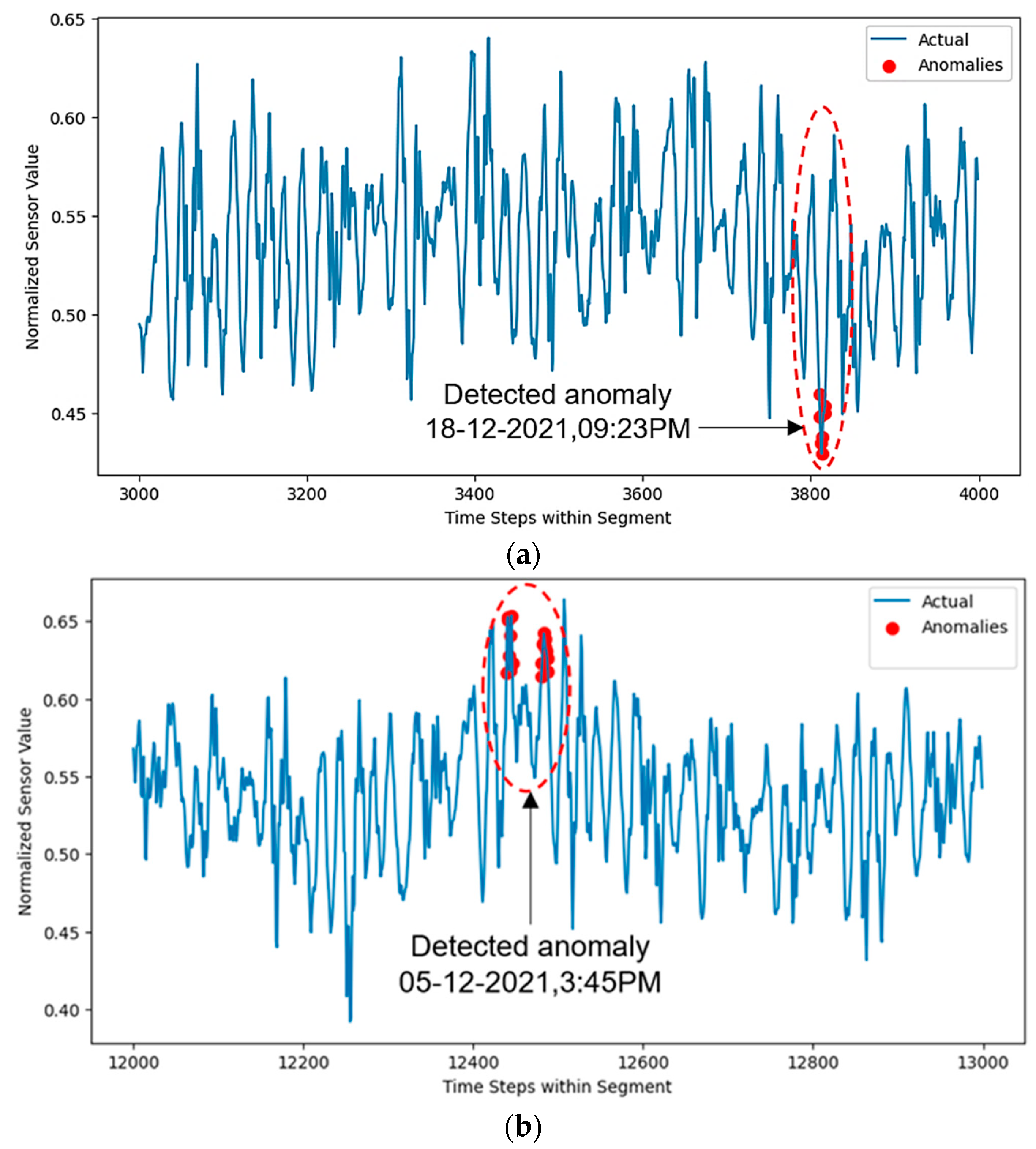
The results reveal that the TCN–Autoencoder exhibited the most promising performance in all three metrics, with an MSE of 1.447, RMSE of 1.193, and MAE of 0.712. This shows that the TCN–Autoencoder excels in accurately reconstructing time-series data and reveals its potential as a robust model for anomaly detection. In contrast, GRU–Autoencoder and LSTM–Autoencoder displayed slightly higher MSE values of 1.824 and 1.822, respectively, along with RMSE values of 1.343 for both models. The MAE for these models was also relatively close, with the GRU–Autoencoder at 0.741 and the LSTM–Autoencoder at 0.725. While these models perform adequately, their results indicate that they may not be as effective as the TCN–Autoencoder in capturing complex patterns in the data. Finally, VAE exhibited an MSE of 1.825, RMSE of 1.343, and MAE of 0.707 when competing. While its performance is similar to the GRU–Autoencoder and LSTM–Autoencoder, it falls slightly behind the TCN–Autoencoder in terms of accurately reconstructing time-series data. Based on our comprehensive evaluation, the TCN–Autoencoder emerges as the most promising choice for time-series anomaly detection with superior performance in terms of MSE, RMSE, and MAE. However, further research and testing may be required to explore the full potential of these models and their application in specific real-world scenarios. In Figure 7, the TCN–Autoencoder model demonstrates its effectiveness in identifying anomalies in the vibration data collected from the Kirkuk power plant. The figure presents two distinct parts where anomalies are encircled with dashed lines, indicating critical deviations from normal operating patterns, and potentially pointing to mechanical issues. Figure 7a presents an anomaly detected during a period of increased load on the turbine. The model identified an unusual pattern that deviated significantly from the baseline vibration sign. Further investigation attributed this to a slight misalignment in one of the turbine blades, exacerbated by load conditions. Such misalignments, if not addressed quickly, can lead to increased wear and tear. Figure 7b depicts an anomaly that coincides with a transient spike in vibration that is accurately captured by the model. This spike is attributed to a temporary obstruction in the air inlet, possibly caused by debris, momentarily disrupting the airflow dynamics inside the turbine.

Figure 7.
The output of the TCN–Autoencoder designed for anomaly detection. The images demonstrate the normalized sensor data over time steps in a segment and highlight two expert-confirmed anomalous events detected by the TCN–Autoencoder. The anomalies are encircled in dashed lines.
The TCN–Autoencoder’s ability to detect these anomalies can be attributed to its architectural features, which include multiple dilated convolutions that help capture a wide range of temporal dependencies in sequential data. The Multi-Head Attention mechanism allows the model to simultaneously focus on different temporal segments of the data, increasing its sensitivity to subtle anomalies indicative of underlying mechanical issues. A detailed breakdown of these anomalies and their origins not only validates the model’s effectiveness but also provides actionable insights for maintenance teams. Early detection of such issues is vital for taking quick actions to prevent costly downtimes and maintain operational efficiency. Blade misalignment (Figure 7a): Detected in the turbine’s compressor blades, misalignment can cause uneven loading of the blades, leading to excessive vibration and potential mechanical failure. This directly affects the efficiency and longevity of the turbine. To avoid the proposed problem, routine visual and instrumental inspections should be performed to check blade alignment and wear. Moreover, the use of dynamic balancing techniques during maintenance cycles to ensure uniform weight and alignment of turbine blades can prevent the aforementioned problem. Air intake obstruction (Figure 7b): This anomaly was traced to the air inlet section of the turbine. Debris or other obstructions can disrupt airflow, causing instability in combustion and increasing operational risks. To avoid the proposed problem based on Figure 7b, implementing the following solutions can help prevent anomalies: (1) Advanced Filtration System: upgrade existing air filtration systems to prevent debris from the intake tracts, (2) Regular Cleaning Schedules: establish strict cleaning schedules for the air inlet area to remove any accumulated debris, and (3) Real-time Monitoring: deploy sensors at strategic points in the air inlet system to monitor for any signs of obstruction or reduced airflow efficiency.
6. Conclusions
This study introduces a novel fault detection algorithm designed for gas turbines using machine learning techniques, specifically a Temporal Convolutional Network (TCN)–Autoencoder model. This model is designed to excel in handling sequential data collected from the Kirkuk power plant utilizing CA 202 accelerometer readings. Comparative analysis with traditional machine learning models commonly employed for time-series anomaly detection, such as the GRU–Autoencoder, LSTM–Autoencoder, and VAE, reveals superior performance in terms of the MSE, RMSE, and MAE. The proposed model demonstrates increased accuracy with a lower MSE (1.447), RMSE (1.193), and MAE (0.712), which emphasizes its effectiveness in enhancing predictive maintenance and operational efficiency in power plants. Future efforts will address further refinements and diverse applications for the proposed model, with the goal of advancing predictive maintenance and operational efficiency across the power plant domain.
Author Contributions
Conceptualization, K.R.K.; methodology, A.-T.W.K.F., K.R.K. and S.G.; software, A.-T.W.K.F.; validation, A.-T.W.K.F.; formal analysis, A.-T.W.K.F. and K.R.K.; investigation, A.-T.W.K.F., K.R.K. and S.G.; resources, A.-T.W.K.F.; data curation, A.-T.W.K.F.; writing—original draft preparation, A.-T.W.K.F. and S.G.; writing—review and editing, K.R.K.; visualization, K.R.K.; supervision, K.R.K. and S.G.; project administration, K.R.K.; funding acquisition, K.R.K. and S.G. All authors have read and agreed to the published version of the manuscript.
Funding
This research received no external funding.
Institutional Review Board Statement
Not applicable.
Informed Consent Statement
Not applicable
Data Availability Statement
The datasets can be made available upon request from the first author.
Acknowledgments
This paper has been supported by the RUDN University Strategic Academic Leadership Program.
Conflicts of Interest
The authors declare no conflicts of interest.
References
- Poullikkas, A. An overview of current and future sustainable gas turbine technologies. Renew. Sustain. Energy Rev. 2005, 9, 409–443. [Google Scholar] [CrossRef]
- Tanaka, K.; Cavalett, O.; Collins, W.J.; Cherubini, F. Asserting the climate benefits of the coal-to-gas shift across temporal and spatial scales. Nat. Clim. Chang. 2019, 9, 389–396. [Google Scholar] [CrossRef]
- Assareh, E.; Agarwal, N.; Arabkoohsar, A.; Ghodrat, M.; Lee, M. A transient study on a solar-assisted combined gas power cycle for sustainable multi-generation in hot and cold climates: Case studies of Dubai and Toronto. Energy 2023, 282, 128423. [Google Scholar] [CrossRef]
- National Academies of Sciences, Engineering, and Medicine. Advanced Technologies for Gas Turbines; National Academies Press: Washington, DC, USA, 2020. [Google Scholar] [CrossRef]
- Meher-Homji, C.B.; Chaker, M.; Bromley, A.F. The Fouling of Axial Flow Compressors: Causes, Effects, Susceptibility, and Sensitivity. In Volume 4: Cycle Innovations; Industrial and Cogeneration; Manufacturing Materials and Metallurgy; Marine, Proceedings of the ASME Turbo Expo 2009: Power for Land, Sea, and Air, Orlando, FL, USA, 8–12 June 2009; ASME: New York City, NY, USA, 2009; pp. 571–590. [Google Scholar] [CrossRef]
- De Michelis, C.; Rinaldi, C.; Sampietri, C.; Vario, R. Condition monitoring and assessment of power plant components. In Power Plant Life Management and Performance Improvement; John, E.O., Ed.; Woodhead Publishing: Sawston, UK, 2011; pp. 38–109. [Google Scholar] [CrossRef]
- Mourad, A.H.I.; Almomani, A.; Sheikh, I.A.; Elsheikh, A.H. Failure analysis of gas and wind turbine blades: A review. Eng. Fail. Ana 2023, 146, 107107. [Google Scholar] [CrossRef]
- Waleed, K.M.; Reza, K.K.; Ghorbani, S. Common failures in hydraulic Kaplan turbine blades and practical solutions. Materials 2023, 16, 3303. [Google Scholar] [CrossRef] [PubMed]
- Fahmi, A.T.W.K.; Kashyzadeh, K.R.; Ghorbani, S. A comprehensive review on mechanical failures cause vibration in the gas turbine of combined cycle power plants. Eng. Fail. Anal 2022, 134, 106094. [Google Scholar] [CrossRef]
- Kurz, R.; Meher, H.C.; Brun, K.; Moore, J.J.; Gonzalez, F. Gas turbine performance and maintenance. In Proceedings of the 42nd Turbomachinery Symposium, Houston, TX, USA, 1–3 October 2013; Texas A&M University, Turbomachinery Laboratories: College Station, TX, 2013. [Google Scholar]
- Sun, J.; Bu, J.; Yang, J.; Hao, Y.; Lang, H. Wear failure analysis of ball bearings based on lubricating oil for gas turbine. Ind. Lubr. Tribol. 2023, 75, 36–41. [Google Scholar] [CrossRef]
- Fentaye, A.D.; Baheta, A.T.; Gilani, S.I.; Kyprianidis, K.G. A review on gas turbine gas-path diagnostics: State-of-the-art methods, challenges and opportunities. Aerospace 2019, 6, 83. [Google Scholar] [CrossRef]
- Volponi, A.J. Gas turbine engine health management: Past, present, and future trends. J. Eng. Gas. Turb Power 2014, 136, 051201. [Google Scholar] [CrossRef]
- Matthaiou, I.; Khandelwal, B.; Antoniadou, I. Vibration monitoring of gas turbine engines: Machine-learning approaches and their challenges. Front. Built Environ. 2017, 3, 54. [Google Scholar] [CrossRef]
- Abram, C.; Fond, B.; Beyrau, F. Temperature measurement techniques for gas and liquid flows using thermographic phosphor tracer particles. Prog. Energ. Combust. 2018, 64, 93–156. [Google Scholar] [CrossRef]
- Goebbels, K.; Reiter, H. Non-Destructive Evaluation of Ceramic Gas Turbine Components by X-Rays and Other Methods. In Progress in Nitrogen Ceramics; Riley, F.L., Ed.; Springer: Dordrecht, The Netherlands, 1983; Volume 65, pp. 627–634. [Google Scholar] [CrossRef]
- Zhu, X.; Zhong, C.; Zhe, J. Lubricating oil conditioning sensors for online machine health monitoring–A review. Tribol. Int. 2017, 109, 473–484. [Google Scholar] [CrossRef]
- DeSilva, U.; Bunce, R.H.; Schmitt, J.M.; Claussen, H. Gas turbine exhaust temperature measurement approach using time-frequency controlled sources. In Volume 6: Ceramics; Controls, Diagnostics and Instrumentation; Education; Manufacturing Materials and Metallurgy; Honors and Awards, Proceedings of the ASME Turbo Expo 2015: Turbine Technical Conference and Exposition, Montreal, QC, Canada, 15–19 June 2015; ASME: New York City, NY, USA, 2015; p. V006T05A001. [Google Scholar] [CrossRef]
- Mevissen, F.; Meo, M. A review of NDT/structural health monitoring techniques for hot gas components in gas turbines. Sensors 2019, 19, 711. [Google Scholar] [CrossRef] [PubMed]
- Qaiser, M.T. Data Analysis and Prediction of Turbine Failures Based on Machine Learning and Deep Learning Techniques. Master’s Thesis, Norwegian University of Science and Technology, Trondheim, Norway, 2023. [Google Scholar]
- Yan, W.; Yu, L. On accurate and reliable anomaly detection for gas turbine combustors: A deep learning approach. arXiv 2019, arXiv:1908.09238. [Google Scholar] [CrossRef]
- Zhong, S.S.; Fu, S.; Lin, L. A novel gas turbine fault diagnosis method based on transfer learning with CNN. Measurement 2019, 137, 435–453. [Google Scholar] [CrossRef]
- Zhou, D.; Yao, Q.; Wu, H.; Ma, S.; Zhang, H. Fault diagnosis of gas turbine based on partly interpretable convolutional neural networks. Energy 2020, 200, 117467. [Google Scholar] [CrossRef]
- Rezaeian, N.; Gurina, R.; Saltykova, O.A.; Hezla, L.; Nohurov, M.; Reza Kashyzadeh, K. Novel GA-Based DNN Architecture for Identifying the Failure Mode with High Accuracy and Analyzing Its Effects on the System. Appl. Sci. 2024, 14, 3354. [Google Scholar] [CrossRef]
- Tang, Y.; Sun, Z.; Zhou, D.; Huang, Y. Failure mode and effects analysis using an improved pignistic probability transformation function and grey relational projection method. Complex. Intell. Syst. 2024, 10, 2233–2247. [Google Scholar] [CrossRef]
- Babu, C.J.; Samuel, M.P.; Davis, A. Framework for development of comprehensive diagnostic tool for fault detection and diagnosis of gas turbine engines. J. Aerosp. Qual. Reliab. (Spec. Issue) 2016, 6, 35–47. [Google Scholar]
- Vatani, A. Degradation Prognostics in Gas Turbine Engines Using Neural Networks. Ph.D. Thesis, Concordia University, Montreal, QC, Canada, 2013. [Google Scholar]
- Lim, M.H.; Leong, M.S. Diagnosis for loose blades in gas turbines using wavelet analysis. J. Eng. Gas. Turbines Power 2005, 127, 314–322. [Google Scholar] [CrossRef]
- Arrigone, G.M.; Hilton, M. Theory and practice in using Fourier transform infrared spectroscopy to detect hydrocarbons in emissions from gas turbine engines. Fuel 2005, 84, 1052–1058. [Google Scholar] [CrossRef]
- Santoso, B.; Anggraeni, W.; Pariaman, H.; Purnomo, M.H. RNN-Autoencoder approach for anomaly detection in power plant predictive maintenance systems. Int. J. Intell. Eng. Syst. 2022, 15, 363–381. [Google Scholar] [CrossRef]
- Farahani, M. Anomaly Detection on Gas Turbine Time-Series’ Data Using Deep LSTM-Autoencoder. Master’s Thesis, Department of Computing Science, Faculty of Science and Technology, Umeå University, Umeå, Sweden, 2021. [Google Scholar]
- Zhultriza, F.; Subiantoro, A. Gas turbine anomaly prediction using hybrid convolutional neural network with LSTM in power plant. In Proceedings of the 2022 IEEE International Conference on Cybernetics and Computational Intelligence (CyberneticsCom), Malang, Indonesia, 16–18 June 2022; pp. 242–247. [Google Scholar] [CrossRef]
- Liu, J.; Zhu, H.; Liu, Y.; Wu, H.; Lan, Y.; Zhang, X. April. Anomaly detection for time series using temporal convolutional networks and Gaussian mixture model. J. Phys. Conf. Ser. 2019, 1187, 042111. [Google Scholar] [CrossRef]
- Fahmi, A.T.W.K.; Kashyzadeh, K.R.; Ghorbani, S. Fault detection in the gas turbine of the Kirkuk power plant: An anomaly detection approach using DLSTM-Autoencoder. Eng. Fail. Anal. 2024, 160, 108213. [Google Scholar] [CrossRef]
- Meggitt PLC. CA202 Piezoelectric Accelerometer, Document Reference DS 262-020 Version 9, 15.06.2021. Available online: https://catalogue.meggittsensing.com/wp-content/uploads/2020/09/CA202-piezoelectric-accelerometer-data-sheet-English-.pdf (accessed on 14 May 2023).
- Guiñón, J.L.; Ortega, E.; García-Antón, J.; Pérez-Herranz, V. Moving average and Savitzki-Golay smoothing filters using Mathcad. Pap. ICEE 2007, 2007, 1–4. [Google Scholar]
- Das, K.; Jiang, J.; Rao, J.N.K. Mean squared error of empirical predictor. Ann. Stat. 2004, 32, 818–840. [Google Scholar] [CrossRef]
- Mylonas, C.; Abdallah, I.; Chatzi, E. Conditional variational autoencoders for probabilistic wind turbine blade fatigue estimation using Supervisory, Control, and Data Acquisition data. Wind. Energy 2021, 24, 1122–1139. [Google Scholar] [CrossRef]
- Reza, K.K.; Amiri, N.; Ghorbani, S.; Souri, K. Prediction of concrete compressive strength using a back-propagation neural network optimized by a genetic algorithm and response surface analysis considering the appearance of aggregates and curing conditions. Buildings 2022, 12, 438. [Google Scholar] [CrossRef]
- Kashyzadeh, K.R.; Ghorbani, S. New neural network-based algorithm for predicting fatigue life of aluminum alloys in terms of machining parameters. Eng. Fail. Anal. 2023, 146, 107128. [Google Scholar] [CrossRef]
- Qi, J.; Du, J.; Siniscalchi, S.M.; Ma, X.; Lee, C.H. On mean absolute error for deep neural network based vector-to-vector regression. IEEE Signal Proc. Let. 2020, 27, 1485–1489. [Google Scholar] [CrossRef]

Disclaimer/Publisher’s Note: The statements, opinions and data contained in all publications are solely those of the individual author(s) and contributor(s) and not of MDPI and/or the editor(s). MDPI and/or the editor(s) disclaim responsibility for any injury to people or property resulting from any ideas, methods, instructions or products referred to in the content. |
© 2024 by the authors. Licensee MDPI, Basel, Switzerland. This article is an open access article distributed under the terms and conditions of the Creative Commons Attribution (CC BY) license (https://creativecommons.org/licenses/by/4.0/).