Abstract
Fast detection of the trajectory is the key point to improve the further emergency proposal. Especially for ultra-long highway, prompt detection is labor-intensive. However, automatic detection relies on the accuracy and speed of vehicle detection, and tracking. In multi-camera surveillance system for ultra-long highways, it is often difficult to capture the same vehicle without intervals, which makes vehicle re-recognition crucial as well. In this paper, we present a framework that includes vehicle detection and tracking using improved DeepSORT, vehicle re-identification, feature extraction based on trajectory rules, and behavior recognition based on trajectory analysis. In particular, we design a network architecture based on DeepSORT with YOLOv5s to address the need for real-time vehicle detection and tracking in real-world traffic management. We further design an attribute recognition module to generate matching individuality attributes for vehicles to improve vehicle re-identification performance under multiple neighboring cameras. Besides, the use of bidirectional LSTM improves the accuracy of trajectory prediction, demonstrating its robustness to noise and fluctuations. The proposed model has a high advantage from the cumulative matching characteristic (CMC) curve shown and even improves above 15.38% compared to other state-of-the-art methods. The model developed on the local highway vehicle dataset is comprehensively evaluated, including abnormal trajectory recognition, lane change detection, and speed anomaly recognition. Experimental results demonstrate the effectiveness of the proposed method in accurately identifying various vehicle behaviors, including lane changes, stops, and even other dangerous driving behavior.
1. Introduction
Computer vision technology has undergone rapid development and has been widely applied in various domains of life [1,2], especially in the field of transportation [3]. This technology enables the identification of vehicles in single-camera scenes, allowing for the extraction of vehicle information such as speed, location, trajectory, and license plate [4,5]. Furthermore, in the context of multi-camera surveillance, it facilitates the association of specific target vehicles, enabling tasks such as vehicle trajectory reconstruction and continuous tracking [6]. Meanwhile, with the advancement of video technology, relying on video to achieve anomalous trajectory identification has the capability to be realised.
Vehicle Track Recognition is a critical technology in the field of traffic management and safety, including the identification of dangerous driving behaviour, abnormal speeds, abnormal parking and dangerous lane changing behaviour, etc. [7]. In real-life traffic environments, anomalies in vehicle trajectories affect the behaviour of the rest of the vehicles, often implying a higher probability of traffic accidents, such as vehicle rollovers, collisions and even casualties. Consequently, achieving accurate and fast identification of abnormal vehicle trajectories can improve travel safety and efficiency.
Currently, most of the existing techniques in this field focus on performance in terms of accuracy, while efficiency considerations are slightly lacking. For example, the DeepSORT [8] algorithm uses a two-stage target detector, R-CNN [9], which is unable to meet the real-time requirements in real-world scenarios. Meanwhile, it is difficult for most of the existing methods to monitor the vehicle’s trajectory throughout the entire journey in ultra-long-distance road scenarios, which makes the automatic identification of trajectory anomalies challenging.
This paper proposes an efficient anomalous trajectory recognition architecture for ultra-long distance highways. We design a network architecture based on DeepSORT with YOLOv5s for efficient multi-vehicle target tracking to quickly acquire trajectories in the visible area. However, there is a certain range of blind spots in the field of view of neighbouring cameras in ultra-long-distance road scenarios, which means that we cannot directly access the vehicle trajectory for the whole journey. To overcome the problem, we apply the Bidirectional LSTM structure to predict the trajectory in the blind area. In addition to this, an attribute recognition module is proposed to efficiently implement vehicle re-identification, which means that we can correctly stitch together the trajectories of the same vehicle on different road sections, and eventually recover the full trajectory of the vehicle.
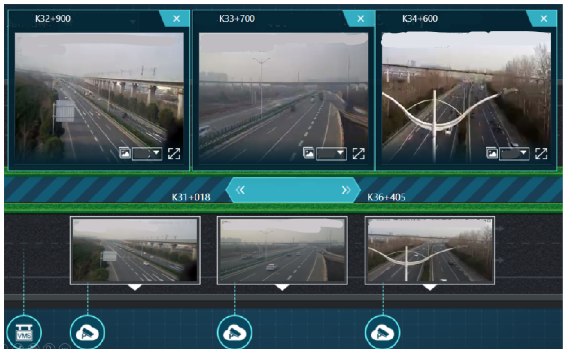
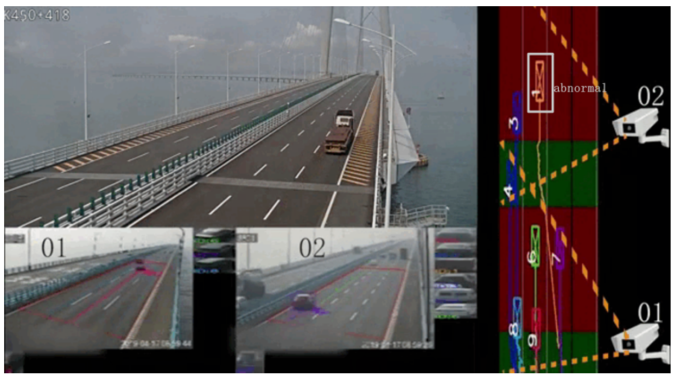
This study selects the Hong Kong-Zhuhai-Macao Bridge Road as the research scenario, aiming to investigate specific situations within highway surveillance videos. In this context, there are short-distance blind spots between various monitoring cameras. To address this limitation, the study employs a driving trajectory integration approach. This involves comprehensive analysis and processing of vehicle trajectory data recorded by monitoring cameras, thereby predicting and outlining the motion trajectories of vehicles within the blind spots. Through this method, the study achieves the stitching and reconstruction of vehicle motion trajectories across the entire area, facilitating the effective identification of abnormal trajectories. Figure 1 shows the experimental scene diagram. The contributions of our paper can be summarized as follows:
1. We proposes an effective framework for vehicle trajectory recognition on ultra-long highways, and designs a network architecture based on DeepSORT and YOLOv5s for efficient multi-vehicle target tracking to quickly obtain trajectories within the visible area.
2. We propose an attribute recognition module to effectively realize vehicle re-identification, correctly splice together the trajectories of the same vehicle on different road sections, and finally restore the complete trajectory of the vehicle. In addition, to solve the problem of a certain range of blind spots between the fields of view of adjacent cameras in ultra-long-distance road scenarios, a bidirectional LSTM structure is introduced in our framework to predict the trajectory of the blind spots.
3. The proposed model was comprehensively evaluated on the Xi’an Ring Expressway re-identification dataset, including abnormal trajectory identification, lane change detection and speed anomaly identification. Experimental results demonstrate the effectiveness of this method in accurately identifying various vehicle behaviors, including lane changing, parking, and even other dangerous driving behaviors.
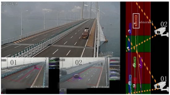
Figure 1.
The experimental scene diagram.
Figure 1.
The experimental scene diagram.
2. Literature Review
The research on highway vehicle tracking technology based on deep learning mainly includes three tasks: vehicle detection, multi-vehicle tracking, and cross-camera vehicle re-identification. This section focuses on the state of the art of related techniques.
2.1. Vehicle Detection and Tracking
Vehicle detection and tracking is divided into two important parts, target detection and multi-target tracking. Target detection is one of the basic problems in the field of computer vision, and is also the core part of many application scenarios, such as face recognition, pedestrian detection, remote sensing target detection, etc. Deep learning-based object detectors can be divided into four categories: two-stage and one-stage object detection according to the network type, and 2D object detection and 3D object detection according to the data type.
The two-stage detection consists of two processes: candidate regions and object classification. In the candidate region stage, the object detector selects a region of Interest (ROI) in the input image containing the target object. In the object classification phase, the most probable ROI is selected, other rois are discarded, and the selected object is classified. Several common detectors are R-CNN, Fast R-CNN [10], and Faster R-CNN [11]. In contrast to two-stage detectors, single-stage object detectors create bounding boxes during object detection and perform classification operations on detected objects. Popular single-stage detectors include YOLO [12], SSD [13], and RetinaNet [14].
For object detection, 2D image data is usually obtained through a 2D object detector. Literature [15] fuses data from radar and camera by learning sensor detection methods. With the booming development of deep learning, researchers are increasingly interested in 3D object detection. Complex-YOLO [16] uses YOLOv2-based Euler Region Proposal Network (E-RPN) to obtain 3D candidate regions.
Multiple object tracking (MOT) is a computer vision task that aims to correlate detected objects across video frames to obtain the entire motion trajectory. In 2016, Bewley et al. [17] proposed the SORT algorithm (Simple Online and Realtime Tracking), which extracts target features in video sequences by combining convolutional neural network and recurrent neural network. Then, the Kalman filter algorithm is used to predict and update the target position, and the Hungarian algorithm is used to realize the data association of the same detection target. Subsequently, Wojke et al. [8] introduced deep learning into the SORT algorithm and proposed the DeepSORT algorithm. By learning the deep feature representation, the convolutional neural network was used to extract the target appearance features to replace the hand-designed features used in SORT. With the development of object detection technology, the original two-stage object detector Faster R-CNN is not so outstanding in the tracking effect in practical application scenarios because of its slow detection speed. Therefore, many replacement object detection algorithms have been proposed to improve the DeepSORT algorithm.
2.2. Vehicle Re-Identification
When a target query graph is given, vehicle re-identification can find out the vehicles with the same ID as the target query graph in the scene of adjacent cameras or several adjacent cameras. With the continuous update and development of deep learning algorithms, this application field has become spectacular. It can be mainly divided into supervised, metric and unsupervised learning methods. Methods based on supervised learning are further divided into methods based on global features [18,19], local features [20,21] and attention mechanism [22]. The goal of metric learning is to learn a mapping from the original features to the embedding space, such that the objects of the same category are close in the embedding space, and the distance between different categories is far away. Euclidean distance and cosine distance are generally used in the distance calculation equation. In the re-identification task based on deep learning method, loss function [23,24] replaces the role of traditional metric learning to guide feature representation learning. In contrast to supervised techniques, unsupervised learning aims to infer directly from unlabeled input data, which addresses the limited generalization ability of models and the high cost of manually labeled data [25]. Shen et al. [23] used clustering features to model global and local features to improve the accuracy of unsupervised vehicle re-identification.
2.3. Abnormal Trajectory Recognition
Microscopic vehicle driving trajectories are closely related to traffic safety analysis. Zhao Youting et al. identified abnormal driving states such as overspeed, low speed and stop based on video detection.
There are many ways to obtain microscopic vehicle driving behavior, including a large number of real event records, driving simulators and microscopic traffic simulation software. Based on obtaining trajectories, the risk factors of traffic accidents can be associated. Among them, Yan et al. [26] systematically studied the relationship between intervention factors and driving behavior safety, providing scientific decision-making basis for traffic safety management. Bao et al. [27] used the trajectory data of floating cars to analyze the colliding-related correlation factors.
Many scholars have studied traffic control to improve safety based on microscopic vehicle trajectory results. Chen et al. [28] studied the traffic safety guarantee technology. Teams such as Tongji University and Jiangsu University also established spatio-temporal correlation analysis between accidents on multi-dimensional risks, laying a foundation for proactive traffic control [29].
Despite the advancements achieved in the field of abnormal trajectory recognition in surveillance videos, several challenges and issues persist. Firstly, there is an ongoing discussion regarding the definition of standards and evaluation metrics for abnormal trajectories. Different scenarios and applications may have varying definitions of abnormality, thus necessitating the establishment of a flexible and universally applicable standard to ensure the suitability and comparability of recognition methods. Additionally, for more accurate algorithm performance evaluation, there is a need to develop finer and more objective evaluation metrics that adequately consider the characteristics of different types of anomalies.
Furthermore, various sources of interference in video data remain a formidable obstacle. Factors such as noise, occlusion, and variations in lighting can disrupt the accurate recognition of abnormal trajectories, necessitating more powerful data preprocessing and enhancement techniques to enhance the system’s robustness against these interferences. Moreover, for cases involving occlusions, exploring data fusion methods from multiple cameras or sensors is essential to obtain more complete and accurate information. Thirdly, real-time performance, scalability, and interpretability are pressing concerns in abnormal trajectory detection methods. Prompt detection of anomalies is crucial in many practical applications, thus necessitating the exploration of efficient algorithms and hardware acceleration techniques for achieving real-time processing. Simultaneously, with the increase in the number of monitoring devices, scalability of the system becomes paramount, requiring the design of algorithms and architectures capable of operating in large-scale environments. Fourthly, the fusion of multimodal information is one of the directions for future development. Utilizing various sources of information such as sound and text allows for a more comprehensive scene analysis and anomaly detection, thereby enhancing overall detection efficacy. However, effectively integrating and jointly analyzing such diverse types of data still warrants further research.
In summary, despite the significant progress achieved in the field of abnormal trajectory recognition in surveillance videos, interdisciplinary collaboration and ongoing research efforts are still required to address the aforementioned challenges and issues, thereby promoting the further advancement and application of this field.
3. Methodology
3.1. Vehicle Detection and Tracking
The algorithm employed in this paper primarily combines YOLOv5s with DeepSORT. In the context of a closed traffic environment such as a highway, achieving real-time vehicle detection under high frame-rate camera surveillance of rapidly moving vehicles necessitates a detection algorithm that is capable of timely processing and minimizes the possibility of overlooking detections in the image sequence. The original DeepSORT model, based on the Tracking-by-Detection (TBD) strategy, utilizes the Faster R-CNN object detection algorithm. While it performs well in accuracy, its processing speed is comparatively slow, rendering it unsuitable for real-time applications. Consequently, this paper integrates the multi-object tracking algorithm, DeepSORT, with the YOLOv5s object detection algorithm to replace Faster R-CNN, thereby enhancing the multi-vehicle tracking performance of the model.
The algorithm comprises two main steps. Firstly, it involves computing the cosine distance of feature vectors and the Mahalanobis distance between detection boxes and prediction boxes using the YOLOv5s network. The computed results are then subjected to weighted fusion to generate an association matrix. Subsequently, the Hungarian algorithm is employed to match vehicle detection boxes with tracking boxes. If a successful match is established, output is generated; if not, a reinitialization of the Kalman filter tracker is required.
3.2. Image-Based Vehicle Re-Identification
The task of vehicle re-identification aims to match the same vehicle across different cameras or time instances through image matching. The key to solving vehicle re-identification lies in feature extraction and similarity measurement computation. Feature extraction based on deep learning is currently the mainstream approach. Similarity measurement typically involves mapping images into a feature space where image similarity can be directly quantified, and then utilizing the extracted feature differences to assess the similarity between two targets. A smaller distance between two targets indicates higher similarity and a higher likelihood of being the same target; a larger distance signifies lower similarity and a lower likelihood of being the same target. Generally, fully connected layers are employed to flatten image features into one-dimensional vectors, followed by the use of suitable distance metrics to compute the disparities between image features. Commonly used distance metrics include Euclidean distance, Manhattan distance, cosine distance, and Mahalanobis distance.
In this paper, when constructing a vehicle re-identification model based on attribute information, the vehicle attribute information extracted from each attribute branch is incorporated into the global features generated by the main network. This incorporation aims to enhance the interaction between attribute features and vehicle re-identification features, thereby producing more distinctive and representative features [30,31].
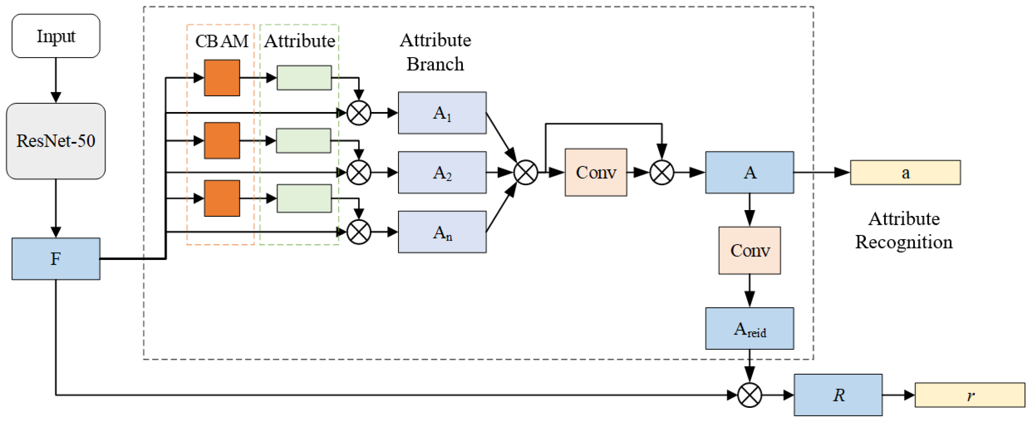
As shown in Figure 2. In the improved vehicle re-identification network architecture focusing on attribute information, the network model first extracts image feature information from the main network, generating a feature map F. Subsequently, the global feature F is fed into attribute branches based on attention modules, resulting in various attribute feature maps . These attribute feature maps are then combined using an attribute re-weighting module to produce a unified and comprehensive attribute feature map A, encompassing all attributes. The generated attribute feature map A undergoes global average pooling and fully connected layers to yield attribute feature vectors for attribute recognition. Simultaneously, useful attribute information is extracted through convolutional operations on the attribute feature map A. This information is subsequently integrated back into the global features, resulting in the final fusion feature map R. The spatial average pooling feature vector r of R is employed for the ultimate vehicle re-identification task.
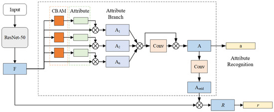
Figure 2.
Architecture diagram of vehicle recognition network based on improved attribute information.
3.3. Anomaly Trajectory Recognition Based on Trajectory Rules
In this paper, anomalous trajectory recognition consists of five main parts: mathematical modelling of vehicle information, mathematical modelling of vehicle behaviour, trajectory acquisition in the visible area, trajectory prediction in the blind area and discrimination of anomalies. Firstly, we model the physical information and driving behaviour of the vehicle to achieve a comprehensive perception of the moving vehicle. After that, vehicle trajectories are acquired and predicted in two actual scene regions (visible region and inside the blind zone), respectively. Finally, according to the defined anomaly rules, the vehicle trajectory is determined as anomalous or not.
3.3.1. Mathematical Description of Vehicle Information
The vehicle trajectory information obtained based on the tracking boxes under a certain surveillance camera includes the following main aspects: the time duration T for which the trajectory exists, the total number of frames f in the trajectory over time T, and the world coordinates of the vehicle’s position in the frame sequence. Generally, z is assumed to be either 0 or a constant. The description of model parameters can be as follows:
- Set of vehicle positions , where ;
- Set of vehicle movement paths , where represents the change in vehicle position, or the path length the vehicle has traveled from the frame to the frame. It is calculated as shown in Equation (1):
- Set of vehicle movement angles , where represents the angle of vehicle movement between the frame and the frame in a coordinate system defined by the coordinates. and is calculated as shown in Equation (2):
- Set of slopes of vehicle movement angles , where represents the slope of the vehicle trajectory from the frame to the frame. It is calculated as shown in Equation (3):
- Set of average vehicle movement speeds , where represents the average speed of the vehicle over the past k frames, from frame to the frame. It is calculated as shown in Equation (4):
In the aforementioned mathematical descriptions, the parameter L can be employed to assess whether the vehicle is in motion, while parameters A and K are utilized to evaluate whether the vehicle’s travel direction is accurate. Additionally, parameter serves to evaluate whether the vehicle’s speed adheres to road regulations.
3.3.2. Mathematical Model of Vehicle Driving Behavior
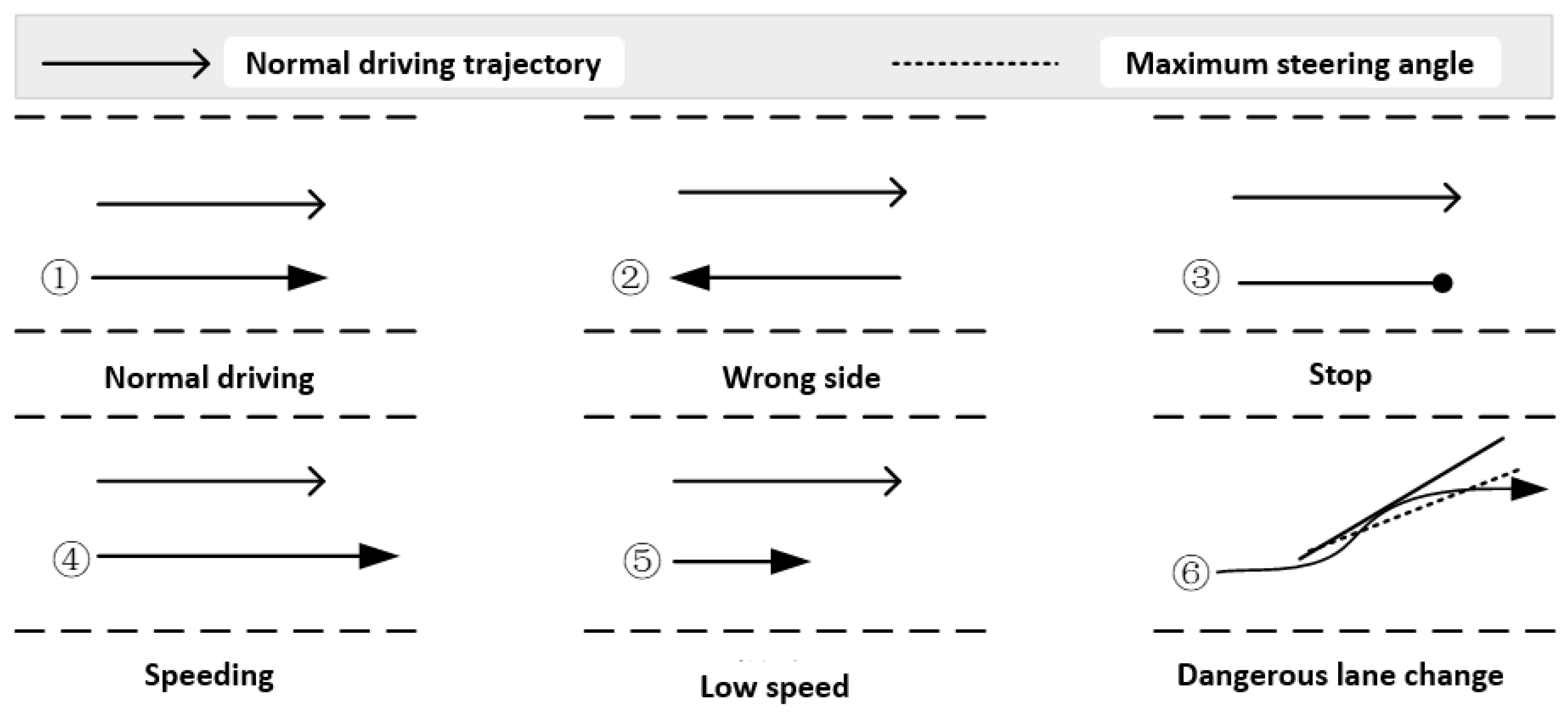
Taking into consideration the characteristics of highway scenarios and vehicle motion, this study categorizes common highway vehicle motion behaviors into normal and abnormal behaviors. Normal behaviors encompass compliant driving actions such as straight-line driving and lane changing that adhere to road traffic safety regulations. Abnormal behaviors, on the other hand, encompass actions like driving in the opposite direction, speeding, moving at a slow pace, stopping, and making hazardous lane changes. A schematic diagram is illustrated in Figure 3 for reference.
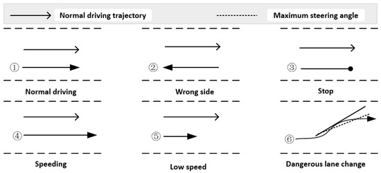
Figure 3.
Schematic diagram of vehicle behavior trajectories for normal behavior and abnormal behavior.
From the vehicle behavior schematic, it can be observed that different abnormal vehicle behaviors correspond to distinct motion characteristics in vehicle trajectories. For a behavior recognition model, key factors to consider include changes in vehicle position, velocity, as well as vehicle motion direction and angles.
We define that vehicles driving in the correct direction according to road regulations, moving away from the camera’s imaging view, are termed “downward”, while those approaching the camera are termed “upward”.
Based on the aforementioned rules and considering the constraints of the application scenario, a mathematical model for vehicle driving behavior can be established. The mathematical model for recognizing downward vehicle behavior is illustrated in Table 1. With the mathematical model of vehicle behavior in place, we can establish a vehicle behavior detection based on trajectory rules to perform behavior detection on the extracted highway vehicle driving trajectories.

Table 1.
Mathematical model for vehicle descent, u represents the threshold for vehicle steering slope, m is the threshold for the minimum allowed speed, and n is the threshold for the maximum allowed speed.
3.3.3. Trajectory Acquisition Method for Visible Scenes
In the visible range of the camera, based on the vehicle tracking results and vehicle modelling information, we can obtain accurate vehicle position information and trajectory on the time series. The positional information of vehicles in camera images is represented in the form of pixel coordinates. These pixel coordinates cannot be directly used to analyze the vehicles’ trajectories in the real-world. Therefore, it is necessary to map the pixel coordinates of vehicles in camera images to their corresponding real-world coordinates, thus obtaining the vehicles’ position information in the real-world. The calculation method between any point in the world coordinate system and its corresponding point in the pixel coordinate system is shown in Equation (5).
In Equation (5), if the pixel coordinates and the world coordinates of any point are known, can be determined as 1. Thus, there remain 11 unknowns in the projection transformation matrix M. In practical scenarios, the bridge deck can be approximated as a horizontal plane in the world coordinate system. The mapping reference points between the pixel coordinate system and the world coordinate system are illustrated in Figure 4.

Figure 4.
Mapping reference points in pixel coordinate system and world coordinate system.
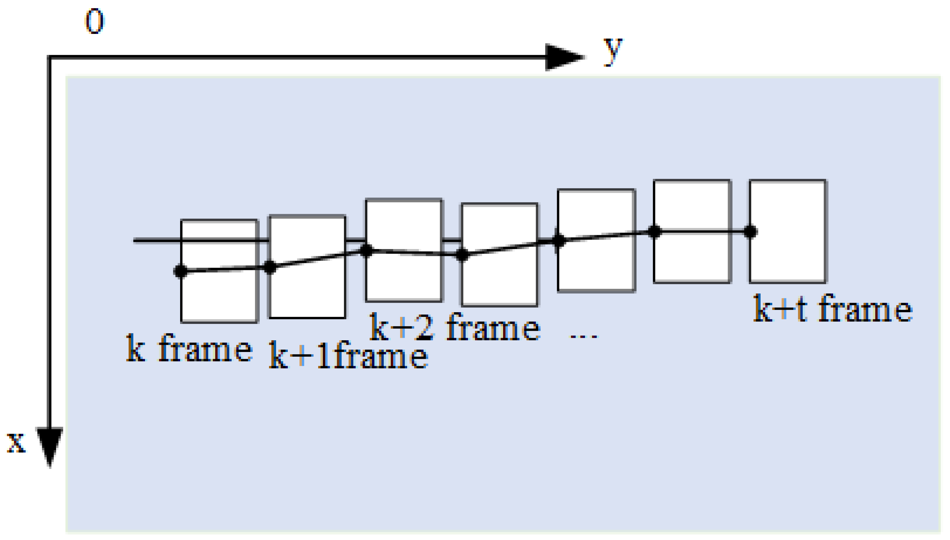
When performing vehicle detection and tracking, precise vehicle location information has already been obtained. After undergoing coordinate transformation, vehicle trajectories can be accurately represented in two-dimensional space. In this section, for the extraction of vehicle trajectories, the collection of bottom center coordinates of the tracked vehicle bounding boxes in each frame is selected as the approximate travel trajectory of the vehicle. The specific process of trajectory extraction can be described as follows: The vehicle bounding boxes detected in the frame are used as the basis for trajectory extraction.
The bottom center coordinates are represented as shown in Equation (6),
where represents the coordinates of the origin, i.e., the upper-left corner of the rectangle, and and denote the width and height of the rectangle, respectively. The obtained trajectory is illustrated in Figure 5.

Figure 5.
Schematic diagram of vehicle movement trajectory.
In the P-th camera view, the trajectory of a certain vehicle in a consecutive sequence of frames can be represented by a sequence of sets containing pixel coordinate points, as shown in Equation (7).
3.3.4. Blind Zone Trajectory Prediction Based on Bidirectional LSTM
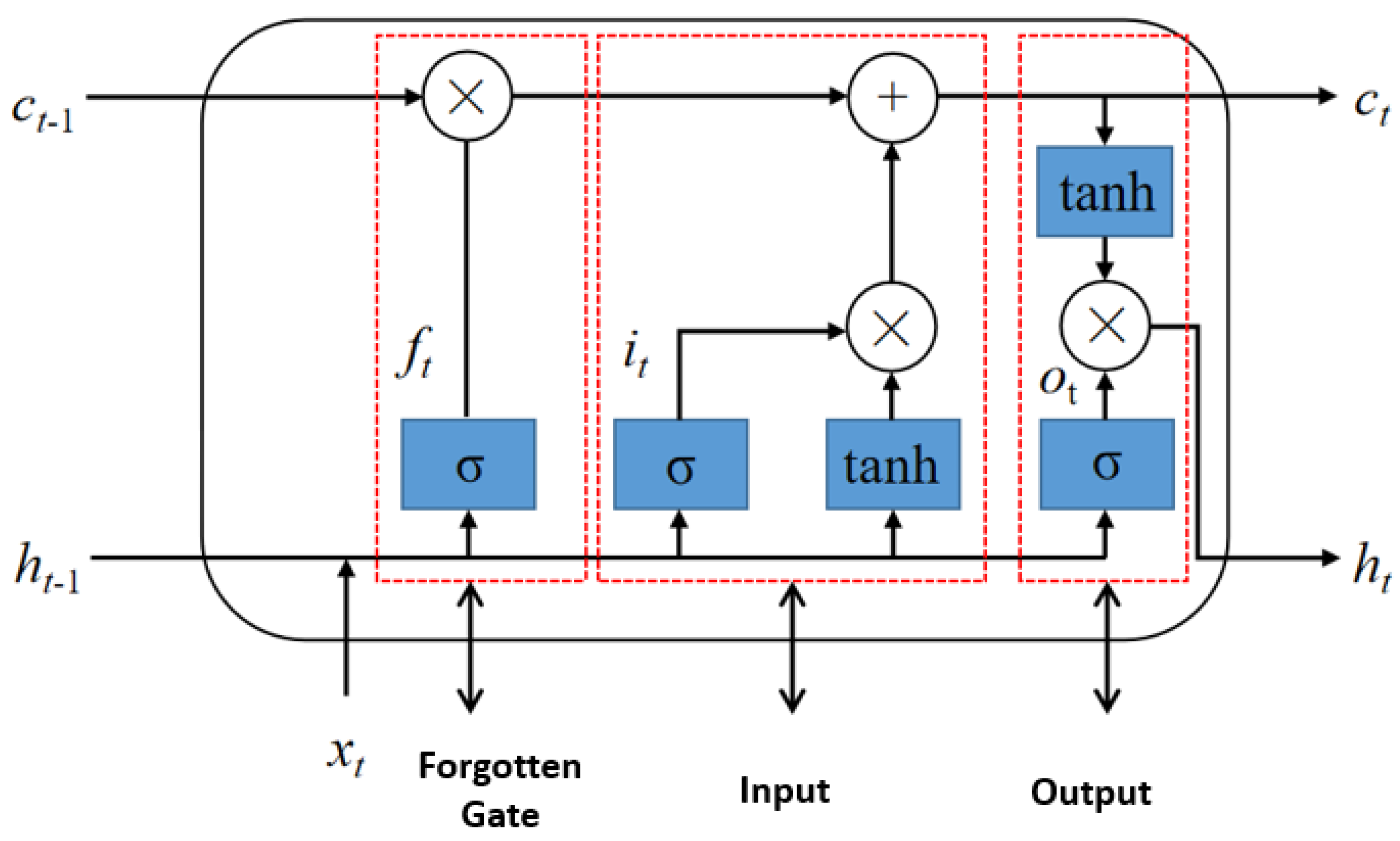
In long-distance tunnels, there is a certain blind spot between multiple cameras, which makes it impossible for us to directly obtain vehicle trajectory information and poses a safety hazard in road traffic management. Long Short-Term Memory (LSTM) is a specialized type of Recurrent Neural Network (RNN) architecture that effectively addresses the vanishing gradient and exploding gradient problems. LSTM incorporates input gates, forget gates, and output gates on top of the basic RNN structure. The architecture of LSTM is depicted in Figure 6.

Figure 6.
LSTM structure diagram. Three input quantities: is the hidden state at the current moment, is the hidden state at the previous moment, and is the unit state at the previous moment. Two output quantities: is the hidden state at the current moment, and is the unit state at the current moment.
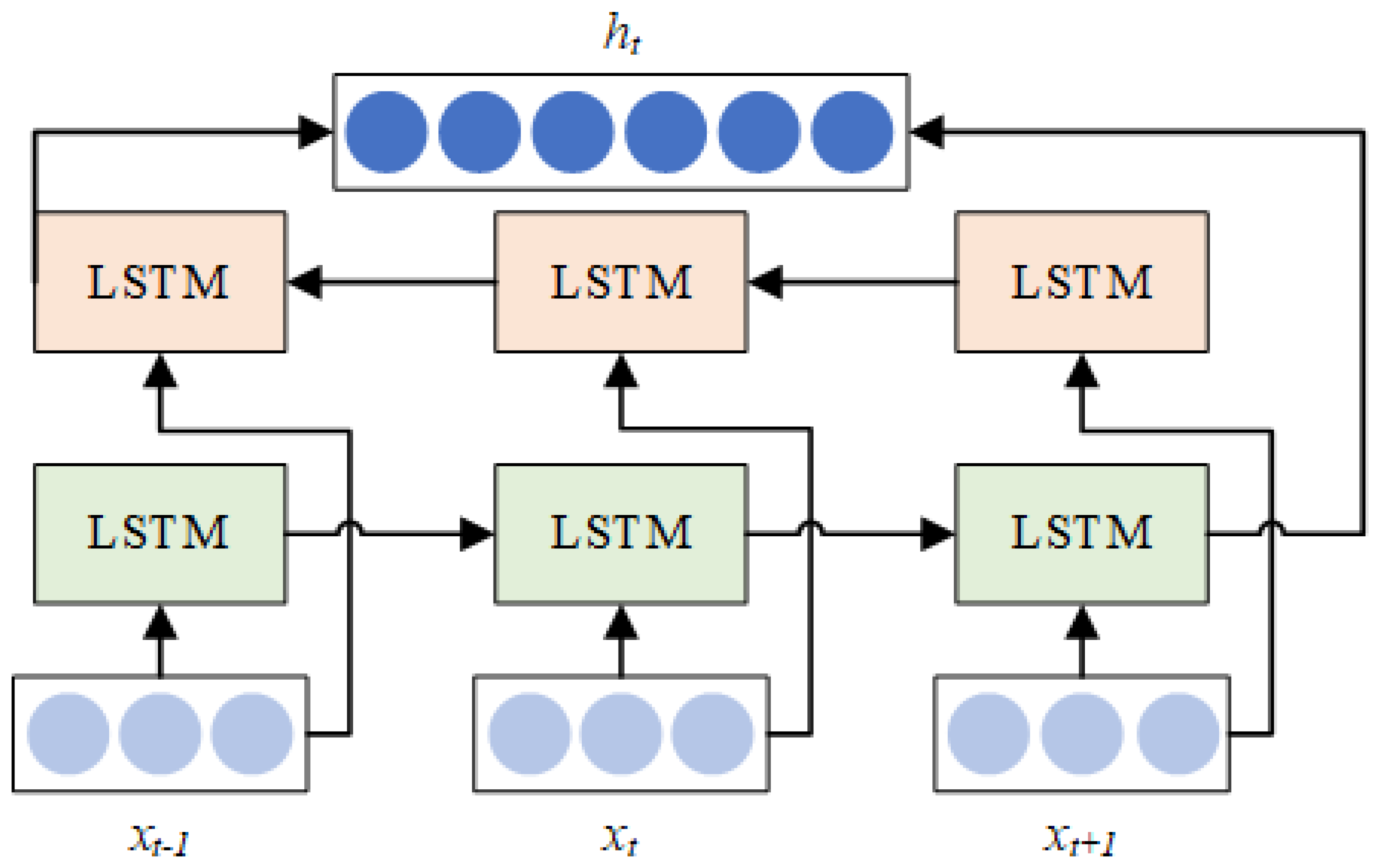
Bidirectional LSTM can simultaneously consider both the forward and backward information of a sequence, thereby enhancing the sequence modeling capability. The network architecture of Bidirectional LSTM is illustrated in Figure 7.
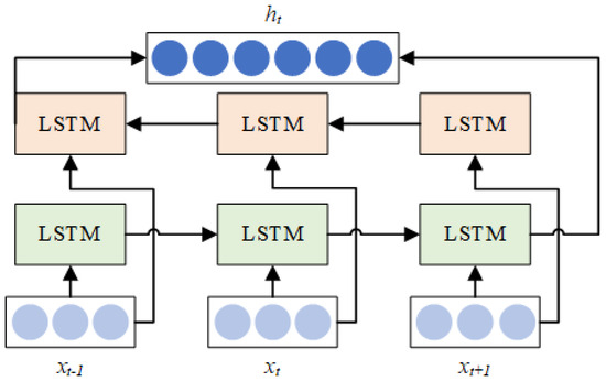
Figure 7.
Bidirectional LSTM structure diagram.
Compared to traditional LSTM, Bidirectional LSTM adds a reverse LSTM layer in its structure. The input sequence is processed separately through the forward and backward LSTM layers, and then the outputs of the two LSTM layers are concatenated along the time dimension. This allows the model to utilize information both before and after the current time step, enabling a more comprehensive sequence modeling and prediction.
During the training of the blind spot vehicle trajectory prediction model based on Bidirectional LSTM, preprocessing is conducted as a preliminary step. The feature sequences, composed of time steps, lateral and longitudinal positions of vehicle trajectories, vehicle speed, acceleration, and other information, are transformed into arrays. Each trajectory’s feature sequence is partitioned into three segments: the front and rear segments are used as inputs, while the middle segment serves as the expected output. Subsequently, the Bidirectional LSTM model is trained. During each forward pass, the hidden parameters of the model are computed, and predictions are generated. The error between the predictions and the ground truth is then calculated, and this error is employed in the backward pass. The model’s various parameters are updated using the principle of gradient descent to minimize the objective function and complete the training process.
3.3.5. Definition of Abnormal Trajectory Rule
In this paper, we mainly define four types of abnormal vehicle trajectory behaviours, which include abnormal driving behaviour, abnormal vehicle speed, abnormal vehicle parking, and dangerous vehicle lane change.
Identification Wrong-way driving behavior: It refers to the abnormal behavior of a vehicle where its actual direction of travel is opposite to the prescribed road direction. Determining wrong-way behavior can primarily involve assessing both the position and angle of vehicle movement. To determine whether a vehicle is engaged in wrong-way driving at frame i, it is first necessary to ascertain whether the set of vehicle movement paths is non-empty. Additionally, it is important to determine whether the monitoring camera is in an upstream or downstream state. Subsequently, the determination of wrong-way behavior is based on the collection of vehicle movement angles. In the downstream state, for normal driving vehicles, as they move away from the camera, the directions of the road regulations, vehicle movement, and the positive y-axis direction of the coordinate calibration are consistent. The range of vehicle movement angles is . A wrong-way frame rate counter Num is set up, where a count is increased by 1 upon detecting a wrong-way frame. When , the vehicle can be classified as performing wrong-way driving. Considering the limited availability of wrong-way datasets, this study employs the opposite upstream/downstream configuration and uses the normal dataset for detecting wrong-way behavior in the reverse direction.
Identification Abnormal vehicle speed behavior: It refers to instances where a vehicle does not adhere to the prescribed speed limit, encompassing both speeding and slow driving. Both of these behaviors pose significant traffic risks in real-world traffic scenarios. In the experiment for detecting abnormal vehicle speed behavior, given the diversity of vehicle types, distinct permissible speed thresholds are applicable. Thus, it is necessary to first determine the current vehicle category and travel lane, and then establish the minimum speed “m” and maximum speed “n” allowed by the road. Subsequently, based on the calculation method for vehicle speed determined during the mathematical description of vehicle trajectories, the vehicle speed is computed to ascertain if abnormal speed behavior is present. Considering the driving characteristics of vehicles in the research scenario, abrupt changes in vehicle speed are unlikely to occur within a brief period. Consequently, simultaneous occurrence of speeding and slow driving anomalies is unlikely. For the calculation, the set of vehicle average speeds “” is computed with k = 10, using the average speed calculation over the most recent 10 frames. A count is incremented by 1 for each instance of speed anomaly. If consecutive 5 frames exhibit speed anomalies, it is concluded that the vehicle is engaged in abnormal speed behavior.
Identification vehicle parking anomalies: In the context of highway scenarios, normal vehicle speeds are extremely high, making parking behavior highly perilous. Although vehicle parking is a continuous process involving gradual speed reduction and slow trajectory changes, we focus solely on identifying the eventual parking outcome. Recognition of parking behavior is achieved by considering the condition where the vehicle’s position no longer changes. We establish a condition of no position change for a consecutive frame sequence of 5 frames. When this time threshold is exceeded, the vehicle is deemed to have parked.
Identification dangerous vehicle lane changes: In the context of highway scenarios, dangerous lane changes are highly hazardous driving behaviors that often result in severe traffic accidents. The occurrence of such behavior typically leads to serious consequences. Rule-based recognition of dangerous lane change behavior is primarily concerned with the vehicle’s steering angle during travel. It mainly detects actions such as U-turns and excessively large steering angles during lane changes that are highly likely to lead to dangerous lane change situations. A threshold value for the vehicle trajectory path slope, denoted as “u” is established. When the path slope exceeds this threshold, it is recognized that the vehicle’s travel direction has deviated significantly from the defined coordinate vertical axis, indicating the presence of a dangerous lane change behavior. The maximum steering angle during a vehicle lane change generally depends on the vehicle’s speed and type.
3.4. Loss Functions
The model augments the feature vector r, which is ultimately utilized for vehicle re-identification, with the triplet loss and the cross-entropy loss . The representation of the feature vector r is depicted as in Equation (8).
In the equation, denotes the global average pooling operation applied to the compensated feature, while and represent the weights and biases of the fully connected layer. This section of the network model is trained based on minimizing the loss function . The computation of the loss function is given by Equation (9).
where is a hyperparameter that balances the importance of the compensated vehicle re-identification loss and the attribute-related loss.
4. Experimental Result
4.1. Construction of Vehicle Detection Datasets
This study constructs a vehicle detection dataset specifically tailored for highway scenarios based on surveillance videos from the road network of Shaanxi Province. The dataset encompasses traffic monitoring videos captured by cameras at different time periods and milepost locations. Image information is extracted from these videos using video processing techniques.
The dataset covers traffic surveillance videos captured by cameras with different pile numbers at different time periods, and image information is extracted by video processing technology. Then, the annotation tool LabelImg is used to label the rectangular boxes of the vehicles in the images of the dataset, and the information such as the type, location and size of the vehicles are annotated. An example of the processing of LabelImg as well as an example of the xml file generated by the final annotation is shown in Figure 8. In this way, a detailed and accurate highway vehicle detection dataset is obtained, which provides strong support for model training.
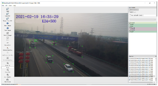
Figure 8.
Use LabelImg to annotate vehicle type, location, and size.
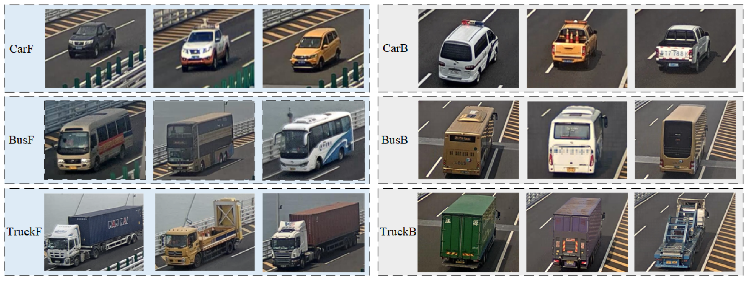
The categorization of the dataset is based on the differences in vehicle shapes and sizes, resulting in three main categories: car, bus, and truck. This categorization to a certain extent mitigates the recognition complexity of the model. Furthermore, considering the varying scales of vehicles captured from different monitoring perspectives, each category of vehicles is further subdivided into two directions: front and rear. The designation “F” is used for vehicles in the front direction, while “B” is used for vehicles in the rear direction. Consequently, the vehicles traveling within the research scene are classified into a total of six categories, as illustrated in Figure 9. In order to maintain the balance of data categories, the number of pictures in each category is 500.
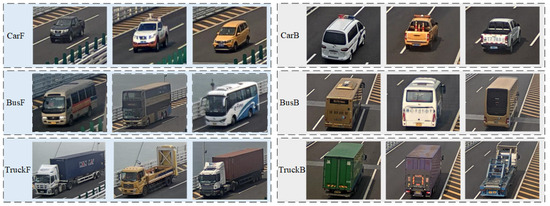
Figure 9.
Vehicles are divided into three categories: cars, buses and trucks, and each category includes two directions of travel.
4.2. Vehicle Detection and Tracking
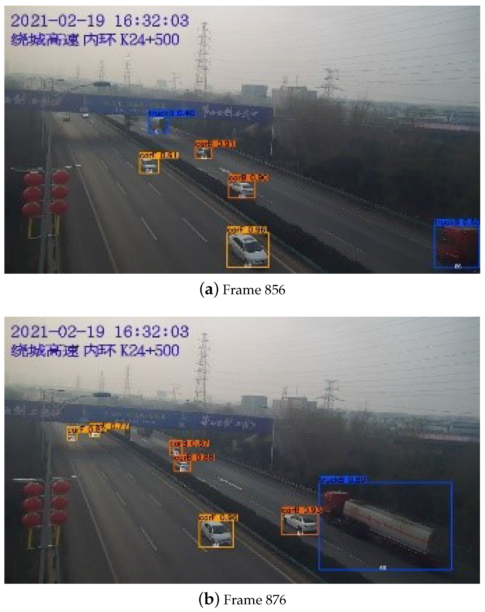
Figure 10 illustrates examples of vehicle tracking in surveillance videos from a camera on a highway in Shaanxi Province. In these examples, the surveillance video has a frame rate of 25 frames per second, and the lower center of the tracking box contains the unique ID of the tracked vehicle.
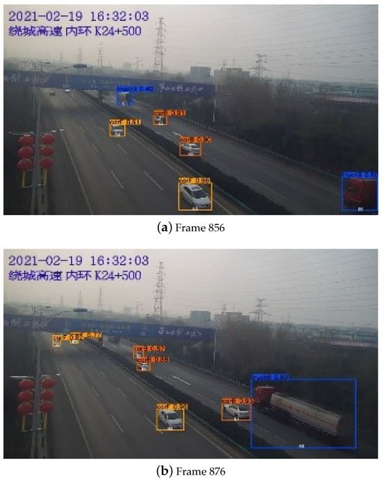
Figure 10.
Example of vehicle tracking effect in real scenes.
The model assigns IDs based on the moment when a vehicle is first tracked. The four displayed images are taken with a time interval of 80 frames, covering most moments when vehicles are captured within the camera’s field of view. From the tracking examples, it can be observed that the improved DeepSORT multi-vehicle tracking model demonstrates effective tracking performance, accurately following and recognizing multiple vehicles.
4.3. Vehicle Re-Identification Based on Image Features
In this chapter, we conducted experiments using the Xi’an Ring Expressway Re-identification Dataset, which was established on the Xi’an Ring Expressway in Shaanxi Province. The purpose of these experiments was to evaluate the robustness of the improved vehicle re-identification model built in this paper.
In the dataset, we collected continuous video footage captured at different time intervals along various mileposts on the expressway. The selected segments have no entrances or exits. A total of 100 vehicles were captured from different perspectives, with milepost locations including K32 + 900, K33 + 700, and K34 + 600 for the upstream direction; and K51 + 610, K51 + 400, K51 + 000, and K50 + 300 for the downstream direction. An example is illustrated in Figure 11.
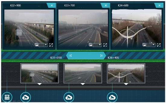
Figure 11.
Schematic diagram of vehicle behavior trajectory.
The comparative algorithms selected for evaluation included models that performed well on the VeRi-776 public dataset, namely: the StRDAN model utilizing attribute-based methods [32], the VAnet model based on viewpoints [33], the PRND model based on vehicle components [34], the SAVER model using GANs [35], and the HPGN model based on graph networks [36]. The Cumulative Matching Characteristic (CMC) curves of the experimental results are shown in Figure 12.
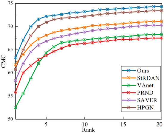
Figure 12.
Cumulative matching characteristic (CMC) curves of different models.
From the results depicted in Figure 12, it is evident that the vehicle re-identification model designed in this chapter, which is based on improved attribute information, outperforms the models utilizing different methods for vehicle re-identification. Furthermore, the experimental results indicate that the vehicle re-identification model based on attribute information exhibits robust performance, making it suitable for the task of re-identifying vehicles across different cameras on the Xi’an Ring Expressway.
4.4. Anomaly Trajectory Recognition Based on Trajectory Rules
In the test set, vehicle trajectories were selected between adjacent cameras that had undergone re-identification to extract trajectories of the same ID. The trajectories were grouped based on predicting and validating the rear 1/2, 1/3, 1/4, and 1/5 lengths of trajectories from the previous camera with corresponding lengths of the front portion of trajectories from the current camera. The error comparison results are presented in Table 2.

Table 2.
RMSE Comparison Results for Trajectory Prediction Experiments.
From the validation error analysis in Table 2, it can be observed that as the prediction distance increases, both the lateral root mean square error and vertical root mean square error continue to grow. However, the vertical root mean square error is larger compared to the lateral root mean square error, attributed to the smaller proportion of vertical distance resolution in pixel coordinates. Overall, the bidirectional LSTM model performs well in predicting vehicle trajectories, with a lateral root mean square error of only 0.56 m and a vertical root mean square error of 1.84 m when half of the trajectory is predicted in both forward and backward directions. The errors between the model’s predictions and actual values are relatively small.
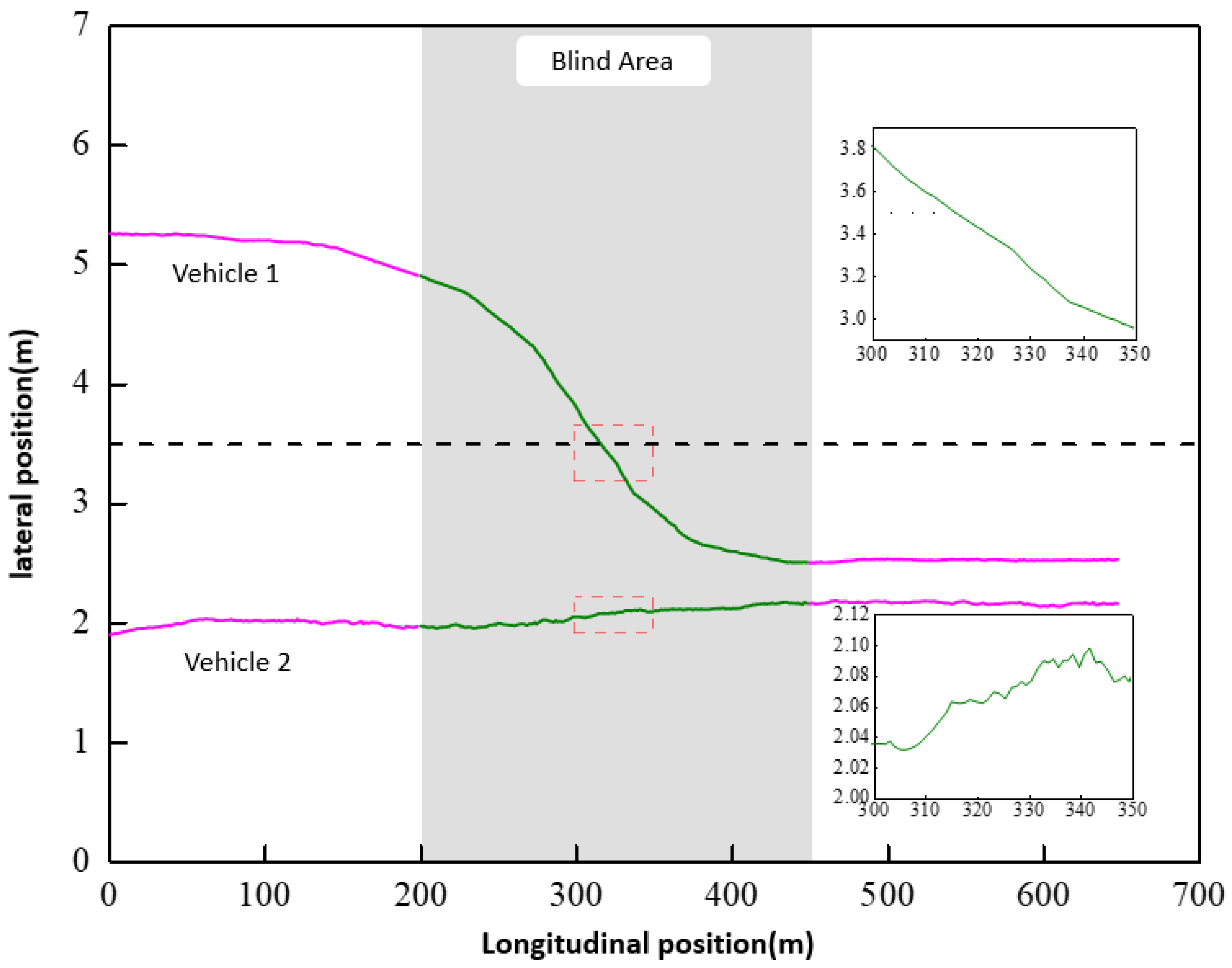
To further enhance vehicle tracking in the context of this study, the blind spot vehicle trajectory prediction model based on bidirectional LSTM was utilized for trajectory concatenation and prediction between adjacent cameras. This approach aimed to obtain complete vehicle travel trajectories under adjacent cameras. Using the Xi’an Ring Expressway as the application scenario, with a camera spacing of 450 m and an effective trajectory length of approximately 200 m per camera, the predicted trajectory length required for the blind spot was about 250 m, accounting for approximately 38.5% of the concatenated complete trajectory. Before concatenation, noise reduction was applied to the vehicle trajectory points by removing points with significant position data fluctuations. The resulting complete vehicle trajectory after concatenation is illustrated in Figure 13.
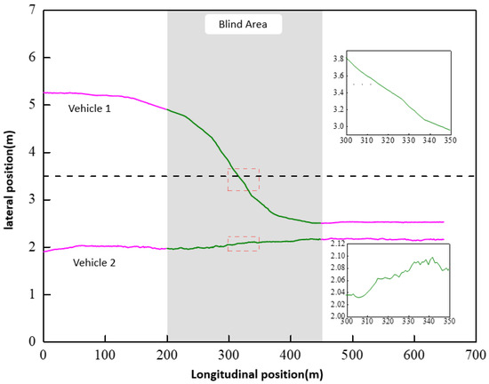
Figure 13.
Schematic diagram of vehicle behavior trajectory.
In Figure 13, the trajectory prediction and concatenation results for two vehicles are displayed. From the overall trajectory prediction results, the predicted trajectories align well with the actual driving behavior of the vehicles. However, due to fluctuations in the obtained vehicle tracking boxes, the predicted trajectories also exhibit a certain degree of fluctuation. Nonetheless, the overall trend remains consistent with normal vehicle driving behavior. This indicates that the trajectory prediction model is capable of effectively handling noise and fluctuations, demonstrating favorable predictive performance.
In Table 3, we quantitatively evaluate the performance of the method in this paper on wrong driving behaviour recognition. It can be seen that the method of this paper correctly identifies the retrograde behaviour on almost all video data.

Table 3.
Statistics of vehicle retrograde behavior recognition results.
Similarly, we quantitatively evaluate the performance of our method on speed anomaly recognition. The experimental results are presented in Table 4 and Table 5. It demonstrates that the methodology of this paper has superior performance.

Table 4.
Statistics of vehicle overspeed behavior identification results.

Table 5.
Statistics of recognition results for slow vehicle behavior.
In the same way, the experimental results for identifying parking behavior of vehicles are presented in Table 6 and for identifying dangerous lane change behavior of vehicles are presented in Table 7. In addition to this, we qualitatively demonstrate the effect of anomalous vehicle detection in a real scenario in Figure 14. It is evident that the method in this paper has excellent performance in the face of multiple vehicle trajectory anomalies.

Table 6.
Statistics of vehicle parking behavior recognition results.

Table 7.
Statistics of recognition results of vehicle dangerous lane change behavior.
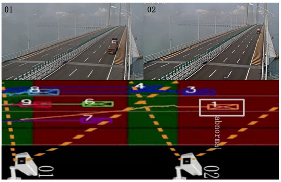
Figure 14.
Real view of abnormal vehicle detection.
5. Discussion
In order to study the highway vehicle tracking technology, the model used in this paper performs well in terms of real-time, accuracy and robustness, and has achieved preliminary research results. However, when dealing with some scenarios with complex traffic conditions or a large monitoring span, the application of these models needs further in-depth research. Specifically, this paper proposes the following three aspects of improvement and perfection:
- The high-speed surveillance video data used in this paper is not perfect, especially the vehicle data for training the vehicle re-identification model in the study scenario is missing. This limits the combination of the deep appearance network for object tracking and the feature extraction network for vehicle re-identification, which increases the complexity of the model to a certain extent. Therefore, future work will further collect relevant data information to improve the model and improve its generalization performance.
- Although the vehicle re-identification method based on attribute information does not need to consider external factors such as spatio-temporal information matching, and only needs to focus on the extraction of the attributes of the vehicle itself, the vehicle behavior detection based on trajectory rules separates the relationship between the vehicle and the surrounding environment and other vehicles when performing trajectory extraction analysis and vehicle abnormal behavior recognition. Therefore, in the subsequent research, the addition of spatio-temporal information of vehicles will be considered, and the deep learning method will be used to cluster and analyze the vehicle trajectory to comprehensively consider the driving behavior of vehicles.
- In this paper, the overall task of highway vehicle tracking is divided into three sub-tasks: vehicle detection, vehicle tracking and vehicle re-identification, and the vehicle trajectory is processed according to the tracking results. The output of the former task is used as the input of the latter task, so the model construction and function implementation are slightly tedious. Therefore, in the subsequent research, we will try to build an integrated model, fuse several models, simplify the model structure, improve the convenience and efficiency of vehicle tracking, and truly realize the global tracking of vehicles on highways, and realize systematization and intelligence.
6. Conclusions
This paper proposes an effective framework for vehicle trajectory recognition on ultra-long highways, and designs a network architecture based on DeepSORT and YOLOv5s for efficient multi-vehicle target tracking to quickly obtain trajectories within the visible area. We also propose an attribute recognition module to effectively implement vehicle re-identification, correctly splice together the trajectories of the same vehicle on different road segments, and ultimately restore the complete trajectory of the vehicle. In addition, to solve the problem of a certain range of blind spots between the fields of view of adjacent cameras in ultra-long-distance road scenarios, a bidirectional LSTM structure is introduced in our framework to predict the trajectory of the blind spots. This study realizes the splicing and reconstruction of vehicle motion trajectories in the entire area, which is conducive to the effective identification of abnormal trajectories. Judging from the Cumulative Matching Characteristic (CMC) curve, the proposed model has high advantages and even improves by more than 15.38% compared with other state-of-the-art methods. Experimental results demonstrate the effectiveness of this method in accurately identifying various vehicle behaviors, including lane changing, parking, and even other dangerous driving behaviors.
Author Contributions
Conceptualization, L.Z.; Methodology, L.Z. and Z.F.; Writing—Original Draft, J.Y.; Writing—Review & Editing, J.Y., Z.Z. and P.W.; Software, L.Z.; Supervision, J.Y. All authors have read and agreed to the published version of the manuscript.
Funding
This work was supported by the Scientific Research Project of Shaanxi Provincial Department of Transportation (No. 21-42X) and Innovation Capability Support Program of Shaanxi (Program No. 2022TD-16).
Institutional Review Board Statement
Not applicable.
Informed Consent Statement
Not applicable.
Data Availability Statement
Dataset available on request from the authors. The raw data supporting the conclusions of this article will be made available by the authors on request.
Conflicts of Interest
Authors Liguo Zhao and Zhipeng Fu were employed by the company CCCC First Highway Consultants Co., Ltd., Xian, China. The remaining authors declare that the research was conducted in the absence of any commercial or financial relationships that could be construed as a potential conflict of interest.
References
- Moshayedi, A.J.; Uddin, N.M.I.; Khan, A.S.; Zhu, J.; Emadi Andani, M. Designing and Developing a Vision-Based System to Investigate the Emotional Effects of News on Short Sleep at Noon: An Experimental Case Study. Sensors 2023, 23, 8422. [Google Scholar] [CrossRef] [PubMed]
- Moshayedi, A.J.; Khan, A.S.; Yang, S.; Zanjani, S.M. Personal Image Classifier Based Handy Pipe Defect Recognizer (HPD): Design and Test. In Proceedings of the 2022 7th International Conference on Intelligent Computing and Signal Processing (ICSP), Xi’an, China, 15–17 April 2022; pp. 1721–1728. [Google Scholar] [CrossRef]
- Chen, H.; Liu, Y.; Zhao, B.; Hu, C.; Zhang, X. Vision-Based Real-Time Online Vulnerable Traffic Participants Trajectory Prediction for Autonomous Vehicle. IEEE Trans. Intell. Veh. 2023, 8, 2110–2122. [Google Scholar] [CrossRef]
- Qi, X.; Zhang, L.; Wang, P.; Yang, J.; Zou, T.; Liu, W. Learning-based MPC for Autonomous Motion Planning at Freeway Off-ramp Diverging. IEEE Trans. Intell. Veh. 2024, 1–11. [Google Scholar] [CrossRef]
- Liu, C.; Huynh, D.Q.; Sun, Y.; Reynolds, M.; Atkinson, S. A Vision-Based Pipeline for Vehicle Counting, Speed Estimation, and Classification. IEEE Trans. Intell. Transp. Syst. 2021, 22, 7547–7560. [Google Scholar] [CrossRef]
- Tang, X.; Zhang, Z.; Qin, Y. On-Road Object Detection and Tracking Based on Radar and Vision Fusion: A Review. IEEE Intell. Transp. Syst. Mag. 2022, 14, 103–128. [Google Scholar] [CrossRef]
- Gao, H.; Qin, Y.; Hu, C.; Liu, Y.; Li, K. An Interacting Multiple Model for Trajectory Prediction of Intelligent Vehicles in Typical Road Traffic Scenario. IEEE Trans. Neural Netw. Learn. Syst. 2023, 34, 6468–6479. [Google Scholar] [CrossRef] [PubMed]
- Wojke, N.; Bewley, A.; Paulus, D. Simple Online and Realtime Tracking with a Deep Association Metric. In Proceedings of the 2017 IEEE International Conference on Image Processing (ICIP), Beijing, China, 17–20 September 2017; pp. 3645–3649. [Google Scholar] [CrossRef]
- Girshick, R.; Donahue, J.; Darrell, T.; Malik, J. Rich feature hierarchies for accurate object detection and semantic segmentation. In Proceedings of the IEEE Conference on Computer Vision and Pattern Recognition, Columbus, OH, USA, 23–28 June 2014; pp. 580–587. [Google Scholar]
- Girshick, R. Fast R-CNN. In Proceedings of the 2015 IEEE International Conference on Computer Vision (ICCV), Santiago, Chile, 7–13 December 2015; pp. 1440–1448. [Google Scholar] [CrossRef]
- Ren, S.; He, K.; Girshick, R.; Sun, J. Faster R-CNN: Towards Real-Time Object Detection with Region Proposal Networks. IEEE Trans. Pattern Anal. Mach. Intell. 2017, 39, 1137–1149. [Google Scholar] [CrossRef] [PubMed]
- Wang, C.Y.; Yeh, I.H.; Liao, H.Y.M. YOLOv9: Learning What You Want to Learn Using Programmable Gradient Information. arXiv 2024, arXiv:2402.13616. [Google Scholar]
- Liu, W.; Anguelov, D.; Erhan, D.; Szegedy, C.; Reed, S.; Fu, C.Y.; Berg, A.C. SSD: Single Shot MultiBox Detector. In Computer Vision—ECCV 2016; Leibe, B., Matas, J., Sebe, N., Welling, M., Eds.; Lecture Notes in Computer Science; Springer: Cham, Switzerland, 2016; pp. 21–37. [Google Scholar] [CrossRef]
- Lin, T.Y.; Goyal, P.; Girshick, R.; He, K.; Dollár, P. Focal loss for dense object detection. In Proceedings of the IEEE International Conference on Computer Vision, Venice, Italy, 22–29 October 2017; pp. 2980–2988. [Google Scholar]
- Guo, Y.; Wang, H.; Hu, Q.; Liu, H.; Liu, L.; Bennamoun, M. Deep Learning for 3D Point Clouds: A Survey. IEEE Trans. Pattern Anal. Mach. Intell. 2021, 43, 4338–4364. [Google Scholar] [CrossRef] [PubMed]
- Simon, M.; Milz, S.; Amende, K.; Gross, H.M. Complex-YOLO: Real-time 3D Object Detection on Point Clouds. arXiv 2018, arXiv:1803.06199. [Google Scholar] [CrossRef]
- Bewley, A.; Ge, Z.; Ott, L.; Ramos, F.; Upcroft, B. Simple Online and Realtime Tracking. In Proceedings of the 2016 IEEE International Conference on Image Processing (ICIP), Phoenix, AZ, USA, 25–28 September 2016; pp. 3464–3468. [Google Scholar] [CrossRef]
- Fu, X.; Peng, J.; Jiang, G.; Wang, H. Learning Latent Features with Local Channel Drop Network for Vehicle Re-Identification. Eng. Appl. Artif. Intell. 2022, 107, 104540. [Google Scholar] [CrossRef]
- Liu, Y.; Zhang, X.; Zhang, B.; Zhang, X.; Wang, S.; Xu, J. Multi-Camera Vehicle Tracking Based on Occlusion-Aware and Inter-Vehicle Information. In Proceedings of the IEEE/CVF Conference on Computer Vision and Pattern Recognition, New Orleans, LA, USA, 18–24 June 2022; pp. 3257–3264. [Google Scholar]
- Zhu, W.; Wang, Z.; Wang, X.; Hu, R.; Liu, H.; Liu, C.; Wang, C.; Li, D. A Dual Self-Attention Mechanism for Vehicle Re-Identification. Pattern Recognit. 2023, 137, 109258. [Google Scholar] [CrossRef]
- Lian, J.; Wang, D.; Zhu, S.; Wu, Y.; Li, C. Transformer-Based Attention Network for Vehicle Re-Identification. Electronics 2022, 11, 1016. [Google Scholar] [CrossRef]
- Bashir, R.M.S.; Shahzad, M.; Fraz, M.M. VR-PROUD: Vehicle Re-identification Using PROgressive Unsupervised Deep Architecture. Pattern Recognit. 2019, 90, 52–65. [Google Scholar] [CrossRef]
- Shen, F.; Du, X.; Zhang, L.; Shu, X.; Tang, J. Triplet Contrastive Representation Learning for Unsupervised Vehicle Re-identification. arXiv 2023, arXiv:2301.09498. [Google Scholar] [CrossRef]
- Chai, X.; Wang, Y.; Chen, X.; Gan, Z.; Zhang, Y. TPE-GAN: Thumbnail Preserving Encryption Based on GAN with Key. IEEE Signal Process. Lett. 2022, 29, 972–976. [Google Scholar] [CrossRef]
- Wu, Y.; Lin, Y.; Dong, X.; Yan, Y.; Ouyang, W.; Yang, Y. Exploit the Unknown Gradually: One-Shot Video-Based Person Re-Identification by Stepwise Learning. In Proceedings of the IEEE Conference on Computer Vision and Pattern Recognition, Salt Lake City, UT, USA, 18–23 June 2018; pp. 5177–5186. [Google Scholar]
- Yan, X.; Xue, Q.; Ma, L.; Xu, Y. Driving-Simulator-Based Test on the Effectiveness of Auditory Red-Light Running Vehicle Warning System Based on Time-To-Collision Sensor. Sensors 2014, 14, 3631–3651. [Google Scholar] [CrossRef] [PubMed]
- Bao, J.; Liu, P.; Qin, X.; Zhou, H. Understanding the Effects of Trip Patterns on Spatially Aggregated Crashes with Large-Scale Taxi GPS Data. Accid. Anal. Prev. 2018, 120, 281–294. [Google Scholar] [CrossRef] [PubMed]
- Chen, J.n.; Zhang, X.; Zhang, S.r.; Jin, Y.I. Comparative Analysis of Parameter Evaluation Methods in Expressway Travel Time Reliability. J. Highw. Transp. Res. Dev. (Engl. Ed.) 2017, 11, 93–99. [Google Scholar] [CrossRef]
- Huang, H.; Chang, F.; Zhou, H.; Lee, J. Modeling Unobserved Heterogeneity for Zonal Crash Frequencies: A Bayesian Multivariate Random-Parameters Model with Mixture Components for Spatially Correlated Data. Anal. Methods Accid. Res. 2019, 24, 100105. [Google Scholar] [CrossRef]
- Lin, Y.; Zheng, L.; Zheng, Z.; Wu, Y.; Hu, Z.; Yan, C.; Yang, Y. Improving Person Re-Identification by Attribute and Identity Learning. Pattern Recognit. 2019, 95, 151–161. [Google Scholar] [CrossRef]
- Quispe, R.; Lan, C.; Zeng, W.; Pedrini, H. AttributeNet: Attribute Enhanced Vehicle Re-Identification. Neurocomputing 2021, 465, 84–92. [Google Scholar] [CrossRef]
- Lee, S.; Park, E.; Yi, H.; Lee, S.H. StRDAN: Synthetic-to-Real Domain Adaptation Network for Vehicle Re-Identification. In Proceedings of the IEEE/CVF Conference on Computer Vision and Pattern Recognition Workshops, Seattle, WA, USA, 14–19 June 2020; pp. 608–609. [Google Scholar]
- Chu, R.; Sun, Y.; Li, Y.; Liu, Z.; Zhang, C.; Wei, Y. Vehicle Re-Identification With Viewpoint-Aware Metric Learning. In Proceedings of the IEEE/CVF International Conference on Computer Vision, Seoul, Republic of Korea, 27 October–2 November 2019; pp. 8282–8291. [Google Scholar]
- He, B.; Li, J.; Zhao, Y.; Tian, Y. Part-Regularized Near-Duplicate Vehicle Re-Identification. In Proceedings of the IEEE/CVF Conference on Computer Vision and Pattern Recognition, Long Beach, CA, USA, 15–20 June 2019; pp. 3997–4005. [Google Scholar]
- Khorramshahi, P.; Peri, N.; Chen, J.c.; Chellappa, R. The Devil Is in the Details: Self-supervised Attention for Vehicle Re-identification. In Computer Vision—ECCV 2020; Vedaldi, A., Bischof, H., Brox, T., Frahm, J.M., Eds.; Lecture Notes in Computer Science; Springer: Cham, Switzerland, 2020; pp. 369–386. [Google Scholar] [CrossRef]
- Shen, F.; Zhu, J.; Zhu, X.; Xie, Y.; Huang, J. Exploring Spatial Significance via Hybrid Pyramidal Graph Network for Vehicle Re-Identification. IEEE Trans. Intell. Transp. Syst. 2022, 23, 8793–8804. [Google Scholar] [CrossRef]
Disclaimer/Publisher’s Note: The statements, opinions and data contained in all publications are solely those of the individual author(s) and contributor(s) and not of MDPI and/or the editor(s). MDPI and/or the editor(s) disclaim responsibility for any injury to people or property resulting from any ideas, methods, instructions or products referred to in the content. |
© 2024 by the authors. Licensee MDPI, Basel, Switzerland. This article is an open access article distributed under the terms and conditions of the Creative Commons Attribution (CC BY) license (https://creativecommons.org/licenses/by/4.0/).

