Modeling of Lane Changing Behavior of Connected Driving Based on Vehicle Interaction Potential

Abstract

Aiming at the interactive behavior of vehicles changing lanes in the intelligent network traffic environment, the relative position of vehicle, speed, acceleration, and steering angle are introduced to correct the molecular interaction potential, and the vehicle interaction potential model is established. The spatial distribution map of the vehicle interaction potential field under different motion states was drawn, and the changing law of the vehicle interaction potential field was described. By analyzing the longitudinal critical distance of the lane changing safe critical time, the expression of acceptable clearance for lane changing is defined, and the relationship between acceptable clearance and the speed and acceleration of the interactive vehicle is verified by simulation. Combined with the acceptable clearance of lane changing, a lane changing behavior model based on the vehicle interaction potential is established, and the situation of lane changing vehicles subjected to the interaction potential and potential field forces generated by the surrounding vehicles is analyzed, and the driving decision of lane changing vehicles under the action of different potential field forces is given. Compared with the molecular dynamics lane changing model and LS2015 lane changing model, the results show that the vehicle action potential lane changing model can effectively improve the running speed and stability of traffic flow. The research has theoretical significance for the lane changing behavior decisions of networked autonomous vehicles in the future.

1. Introduction

Lane changing is one of the main behaviors in vehicle driving and one of the main causes of road traffic accidents. Compared with following behavior, lane changing behavior has a higher complexity. With the development of intelligent network technology, real-time driving information can be obtained between vehicles and vehicles and between vehicles and the road environment, which puts forward higher requirements for the research of vehicle lane changing behavior. Vehicles can achieve the transmission and integration of traffic information through vehicle-to-vehicle communication and vehicle-to-road communication, and conduct real-time driving behavior judgment and operation to ensure driving efficiency and safety.

Vehicle lane changing behavior is a complex decision-making process. In the study of lane changing behavior, Gipps [1] first constructed a vehicle lane changing model framework, which laid a theoretical foundation for subsequent lane changing research. According to the type of lane changing, Erik [2] divides the lane changing behavior into three types: free lane changing, forced lane changing, and collaborative lane changing. In the study of lane changing safety conditions, Ahmed et al. [3] used the gap acceptance model to describe the execution of lane changing behavior and established the lane changing model of forced lane changing and judged lane changing. Jia Hongfei et al. [4] introduced the mutual cooperation mechanism into the lane changing process and established a gap acceptance model considering the characteristics of drivers. Xu Lunhui et al. [5] modeled and analyzed the acceptable clearance of lane changing vehicles and surrounding conflicting vehicles, and fully considered the following safety of lane changing vehicles after lane changing. Wang Chonglun [6] proposed a new acceptable gap model based on different speeds and different driver types. In view of the mutual interference between vehicles in a multi-lane, Shang Lei et al. [7] established the influence model of neighboring vehicles.

As for the research of the potential field, the trajectory planning method of mobile robot based on the artificial potential field concept was first proposed by Khatib [8]. With the development of intelligent transportation, many scholars have extended potential field theory to the field of traffic flow. Based on the gravitational and repulsive fields established by Khatib, Gao et al. [9] proposed a real-time autonomous vehicle controller based on machine learning. Wolf et al. [10] established potential field models for different objects based on artificial potential field theory. Li Linheng et al. [11] improved the existing safe potential field model by introducing acceleration parameters and established the safe potential field lane changing model.

As for the data set used in the research, the data used can be roughly divided into three types: a natural data set, video observation data, and simulation test data. For example, Bham [12] used NGSIM data to investigate gap acceptance behavior during lane changes on highways. Yang et al. [13] used five GM light vehicles equipped with the SHRP2 NextGen data acquisition system to collect real-world driving data and use it for empirical analysis. Due to the limitations of equipment conditions and other aspects, some scholars use simulation experiment platforms, including Prescan 8.5 software [14], to build models of traffic scenes and vehicle control systems.

It is not difficult to see that both the research on the safe distance and the research on the safe potential field are related to the safety during lane changing. Therefore, in the study of lane changing in the intelligent network environment, the influence of the motion parameters of interactive vehicles in the surrounding environment on lane changing safety should be fully considered, and the safety risks that vehicles may cause to lane changing vehicles under different motion states should be analyzed, so as to find a lane changing decision algorithm with simple models and strong applicability to avoid accidents.

Besides the introduction of the first section, there are three sections in this paper. The second section describes the molecular interaction potential model in detail, and then introduces modified parameters to improve the vehicle interaction potential model. By drawing the spatial distribution of the vehicle interaction potential field under different states, it is shown that the modified model is more in line with the actual vehicle operation. When the vehicle interaction potential model is applied to the study of following behavior, it is necessary to calibrate the safe distance between two vehicles. In order to apply the vehicle interaction potential model to lane changing behavior, the acceptable gap between lane changing vehicles and interacting vehicles is studied in the third section. The acceptable gap of lane changing is applied to the vehicle interaction potential model, and the vehicle interaction potential lane changing model is constructed. The fourth section verifies the rationality of the formula of acceptable clearance of lane change, and then verifies the validity of the model by comparing the average speed and average acceleration of traffic flow with simulation tests of different lane change models. The purpose of this paper is to seek a lane change model that is more in line with vehicle driving practice through the study of a vehicle action potential lane change model, to provide new ideas for the study of the lane change behavior of vehicles in an intelligent network environment, and to provide theoretical support for the lane change decisions of connected vehicles.

2. Research of Vehicle Interaction Potential Based on Lennard-Jones Potential

2.1. Vehicle Interaction Potential Based on Lennard-Jones Potential

The molecular force between molecules is the attraction and repulsion interaction between molecules, which is the main reason for the different physical properties of molecules. The equilibrium distance is denoted as the zero distance of the resultant force of molecular attraction and repulsion. When the distance between molecules is greater than the equilibrium distance, the intermolecular force as a whole appears as gravity. When the distance between molecules is less than the equilibrium distance, the intermolecular force as a whole behaves as a repulsive force.

The motion of the traffic flow is reduced to the level of particles; just like the current particle is pushed by the particles behind and pulled by the particles in front of the forward movement, the vehicles are not easy to get close to and not easy to stay away from, and from the dynamic point of view the movement is under the combined action of gravity and repulsion. The interaction between vehicles on the road has similar characteristics to the mechanical relationship between molecules. In this paper, microscopic vehicles in traffic flow are compared to molecules, and a vehicle interaction potential model is established on the basis of molecular dynamics.

The Lennard-Jones molecular action potential function is widely used in modeling research based on molecular dynamics. Based on the intermolecular Lennard-Jones potential, Li Juan [15] established a molecular interaction potential model between following vehicles:

$$U=4\epsilon \left[{\left(\frac{X_r}{L}\right)}^{12}-{\left(\frac{X_r}{L}\right)}^6\right]$$

(1)

where: $\epsilon$ is the depth of the potential well; $L$ is the distance between the front and rear cars; and $X_r$ is the required safe distance for following.

However, 6–12 potential is only a special form of Lennard-Jones potential. Although it conforms to the interaction between microscopic particles in fluids, it is directly applied to the interaction behavior of real vehicles, ignoring the large differences in mass, velocity, and acceleration of the objects studied in the two scenarios. The model results in a strong sensitivity of the vehicle to each parameter. Therefore, Qu Dayi [16] sets the powers of gravitational and repulsive forces in the original model as undetermined parameters, and the vehicle interaction potential function is constructed.

$$U=\frac{\epsilon }{v-u}\left[u{\left(\frac{X_r}{L}\right)}^v-v{\left(\frac{X_r}{L}\right)}^u\right]$$

(2)

where: $v$ and $u$ are powers of the gravitational and repulsive force terms, and $v>u$.

The research shows that when the actual distance between two vehicles is less than the required safety distance, different degrees of short-range repulsion are displayed. The closer the distance, the greater the repulsive force. The contour projection state of the potential field, as shown in Figure 1, indicates that the risk of approaching the vehicle from any direction is the same, but this is obviously unreasonable.

Therefore, consider the following factors that may affect the vehicle potential distribution to modify the model. (1) In the actual road driving environment, the action potential of vehicles at the front and rear of the same lane on the target is significantly higher than that of vehicles in adjacent lanes approaching from the side; (2) dynamic vehicles should show a different acting potential to static vehicles.

The coordinate system is established with the position of the leftmost lane line of the road as the Y axis, as shown in Figure 2.

Taking distance, velocity, and longitudinal acceleration into account in the correction of the model, the vehicle action potential function is obtained as follows:

$$\left\{\begin{array}{c}\begin{array}{l}U=\frac{\epsilon }{v-u}\left[u{\left(\frac{X_r}{L}\right)}^v-v{\left(\frac{X_r}{L}\right)}^u\right]·\exp \left(a\cos \varphi \right)·\frac{d^{\ast }}{\left|d^{\ast }\right|}\\ \end{array}\\ \left|d^{\ast }\right|=\sqrt{{\left[s_0(x-x_0)\right]}^2+{\left[\frac{s_0}{\exp \left(\gamma X_r\right)}(y-y_0)\right]}^2}\end{array}\right.$$

(3)

where: $a$ is vehicle acceleration; $d^{\ast }$ is the corrected distance; $\varphi$ is the clockwise angle formed by vehicle acceleration $a$ and the connection between the two vehicles’ centroids; $s_0$ is the acceptable parking gap; $\gamma$ is undetermined coefficients; the center of mass coordinate position of the current vehicle is $\left(x_0,y_0\right)$, and the center of mass position of any vehicle around is $\left(x,y\right)$; and the meanings of other parameters are the same as those above.

The model is applicable in following behavior, but in the process of lane changing, the vehicle has a certain steering angle, and the spatial distribution of the potential field of the vehicle should also be theoretically deflected as a whole, which cannot be well represented by the above formula. Therefore, the steering angle is introduced to correct Formula (3). $\left(x,y\right)$ is the original coordinate of any vehicle, and $\left(x^{\ast },y^{\ast }\right)$ is the corrected deflection angle coordinate:

$$\left[\begin{array}{l}{x}^{\ast }\\ y^{\ast }\end{array}\right]=\left[\begin{array}{cc}\cos \theta & \sin \theta \\ -\sin \theta & \cos \theta \end{array}\right]\left[\begin{array}{l}x\\ y\end{array}\right]$$

(4)

Combined with Formulas (3) and (4), a vehicle interaction potential model suitable for lane changing behavior is constructed:

$$\left\{\begin{array}{cc}\hfill U& =\frac{\epsilon }{v-u}\left[u{\left(\frac{X_r}{L}\right)}^v-v{\left(\frac{X_r}{L}\right)}^u\right]·\exp \left(a\cos \varphi \right)·\frac{d^{\ast }}{\left|d^{\ast }\right|}\hfill \\ & \left|d^{\ast }\right|=\sqrt{{\left[s_0(x-x_0)\right]}^2+{\left[\frac{s_0}{\exp \left(\gamma X_r\right)}(y-y_0)\right]}^2}\hfill \\ & \left[\begin{array}{l}{x}^{\ast }\\ y^{\ast }\end{array}\right]=\left[\begin{array}{cc}\cos \theta & \sin \theta \\ -\sin \theta & \cos \theta \end{array}\right]\left[\begin{array}{l}x\\ y\end{array}\right]\hfill \end{array}\right.$$

(5)

2.2. Vehicle Potential Field Distribution under Different States

When the distance between vehicles is less than the required safety distance, it is represented as a short-range repulsive force. The potential field of vehicles under different moving states is projected onto the plane to draw its potential field contour diagram, as shown in Figure 3.

Taking the center of mass of the research vehicle as the origin point, the contour lines of the vehicle potential field under the five motion states of stationary, constant speed, acceleration, deceleration, and steering are shown, respectively. The color represents the difference in the size of the potential field, which is white near the center of mass, indicating that the potential field approaches infinity, which means that a vehicle is bound to collide when it appears at this position. This is in line with practical significance. The following analyzes the spatial distribution of the vehicle potential field according to the above five driving states.

(1)

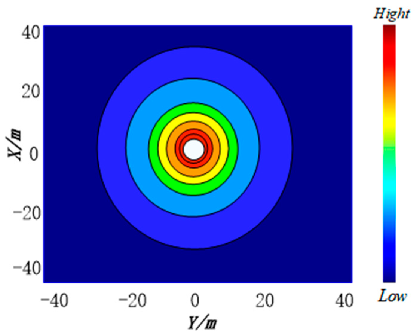
Static state. Figure 3a shows the vehicle at rest, when the vehicle is equivalent to a stationary obstacle. Because the risk of approaching the vehicle from the front and rear is greater than that of approaching the vehicle from the side, the distance is corrected in this paper, so the potential field as a whole is oval.

(2)

State of uniform velocity. Figure 3b,c show the scene when the vehicle is traveling at a constant speed $v=10 \mathrm{m}·{\mathrm{s}}^{-1}$ and $v=15 \mathrm{m}·{\mathrm{s}}^{-1}$ along the axes $y$. comparing Figure 3b,c, it can be found that the potential field increases with the increase in speed in the direction of the vehicle. This also well reflects that the vehicle at high speed has a larger risk range for interactive vehicles than that at low speed. Therefore, the potential field as a whole presents an oval shape elongated along the direction of vehicle motion.

(3)

Accelerated state. Figure 3d,e show a vehicle with a speed of $v=10 \mathrm{m}·{\mathrm{s}}^{-1}$ accelerating along the axes $y$ with $a=1.5 \mathrm{m}·{\mathrm{s}}^{-2}$ and $a=2 \mathrm{m}·{\mathrm{s}}^{-2}$ accelerations, respectively. By comparison with Figure 3b, it can be found that the potential field of the vehicle presents an obvious forward-leaning phenomenon under accelerated motion. This means that the risk to the vehicle in front of the vehicle is significantly greater than that of the vehicle behind, so the required safety distance in front of the vehicle should be greater than that behind the vehicle. By comparing Figure 3d,e, it can be found that with the increase in acceleration, the degree of forward tilt of the vehicle potential field increases. It indicates that the greater the acceleration of the vehicle, the greater the risk to the front.

(4)

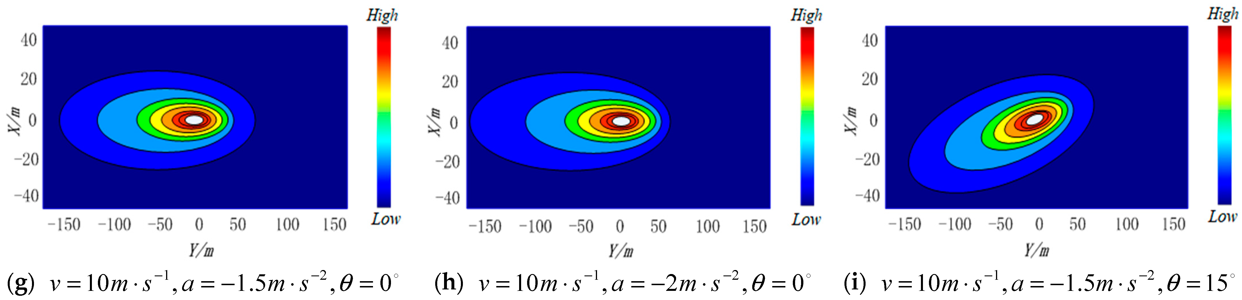
Deceleration state. Figure 3g,h shows the scenario of a vehicle with a speed of $v=10 \mathrm{m}·{\mathrm{s}}^{-1}$ decelerating along an axis with an acceleration of $a=-1.5 \mathrm{m}·{\mathrm{s}}^{-2}$ and $a=-2 \mathrm{m}·{\mathrm{s}}^{-2}$, respectively. By comparison with Figure 3b, it can be found that the potential field of the vehicle shows an obvious backward tilt in the decelerating motion state. This means that the vehicle poses a significantly greater risk to the vehicle behind than to the vehicle in front. So the required safety distance behind the vehicle should be greater. By comparing Figure 3g,h, it can be seen that the potential field of the vehicle increases with the increase in the deceleration value, that is, the risk degree of the rear vehicle increases with the increase in the deceleration speed. Therefore, in the network environment, when the rear vehicle obtains the deceleration information of the front vehicle, it can decelerate in advance to improve driving safety.

(5)

Turning state. Figure 3f,i show the vehicle turning to the left while accelerating and decelerating, respectively. By comparing Figure 3e,h, it can be found that the vehicle potential field as a whole shifts with the steering angle when the vehicle is turning. Therefore, when studying lane changing, it is necessary to consider the influence of the steering angle on the vehicle potential field, which is also in line with the previous revision of vehicle potential field.

3. Acceptable Clearance for Lane Changing

In following behavior, the vehicle only needs to consider the vehicle action potential generated by the vehicles in the same lane, and the two vehicles can drive safely as long as they ensure a certain safe distance from the following demand. However, when the longitudinal repulsive force is not zero, it means that the leading vehicle in the current lane exerts pressure on the target vehicle, and the target vehicle needs to slow down to maintain a safe distance from the leading vehicle. If the vehicle is traveling below the desired speed, a lane changing intention is generated.

When conducting lane changing research, it is necessary to analyze whether the target vehicle and the interacting vehicle meet the safety gap of lane changing. The research shows that the vehicle action potential is the smallest when the acceptable gap of lane changing is satisfied, and the attractive and repulsive forces are zero at this time, and the equilibrium state of lane changing behavior is reached. That is to say, in the case of meeting the acceptable clearance, it can ensure that the vehicle does not slow down and change lanes. Therefore, the acceptable gap in lane changing behavior needs to be studied in the following paragraphs.

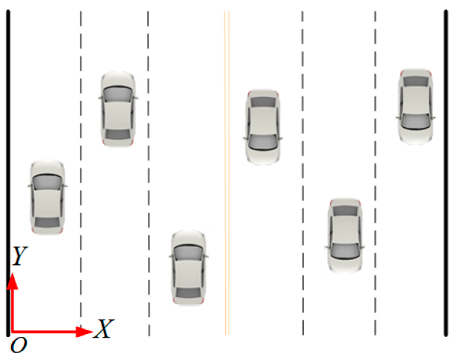
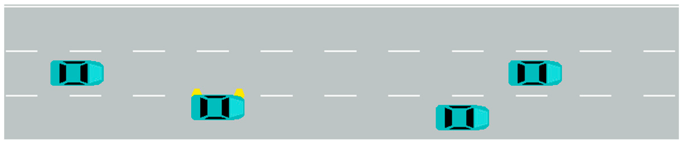
3.1. Study the Setting of the Lane Changing Scene

Lane changing occurs when the driver is eager to achieve a higher speed or more comfortable driving conditions in the adjacent lane, and to reach the destination through diversion or confluence. In general, researchers have divided vehicle lane changing behavior into two categories, forced lane changing and active lane changing, the former of which is performed when the driver must leave the current lane in order to reach the planned destination; when the driver wants to achieve a faster driving speed or a shorter queue, he or she makes an active lane change.

In this paper, active lane changing behavior is selected for analysis. Vehicle lane changing must meet two conditions: First, the speed space advantage; the vehicle in the lane cannot follow the expected speed, and at this time the adjacent lane driving conditions are better. The second is the safety condition of lane changing, which means that the vehicle that is changing lane needs to meet a certain safety distance to avoid traffic accidents.

In the process of lane changing, the traffic safety of the lane changing vehicle M is affected by the traffic flow condition of the surrounding environment, as shown in Figure 4. The research assumes that only four vehicles adjacent to the main vehicle M are considered, in which vehicle L is the vehicle in front of the current lane, F is the vehicle behind the current lane, TL is the vehicle in front of the target lane, and TF is the vehicle behind the target lane. Among the four adjacent vehicles, the rear vehicle F of the original lane and the main vehicle M are in the following state, and the safety relationship between the rear vehicle F of the original lane is mainly determined by the rear vehicle F, so the influence of the rear vehicle F of the original lane is not considered here. In the process of lane changing, the main vehicle M needs to perceive and judge the motion state of the three vehicles L in front of the lane and TL and TF in front of the target lane, and then make decisions and perform operations in a very short time. In this study, the distance where the interaction potential of interacting vehicles is zero during lane changing is called the acceptable gap of lane changing. The following research focuses on the conditions for safe lane changing between lane changing vehicles M and L, and TL and TF.

To simplify the model, the following assumptions are proposed:

(1)

The overall running speed of the target lane is better than that of the current lane, which meets the speed space advantage in lane changing conditions;

(2)

The lane changing vehicle remains in the same state during the lane changing process;

(3)

The influence of steering angle on speed is ignored.

3.2. Research on Acceptable Clearance of Lane Changing

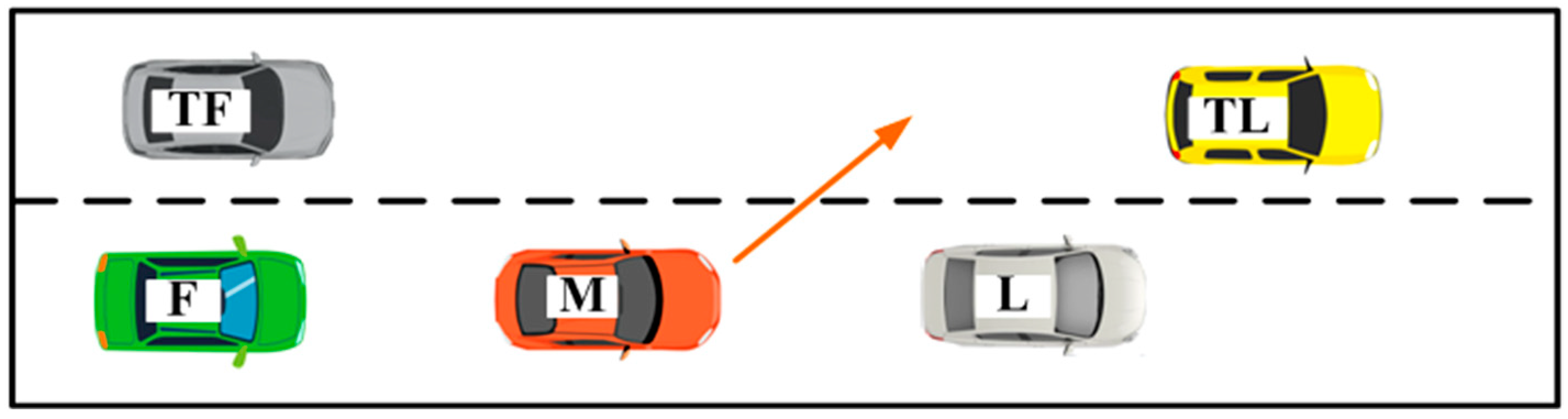
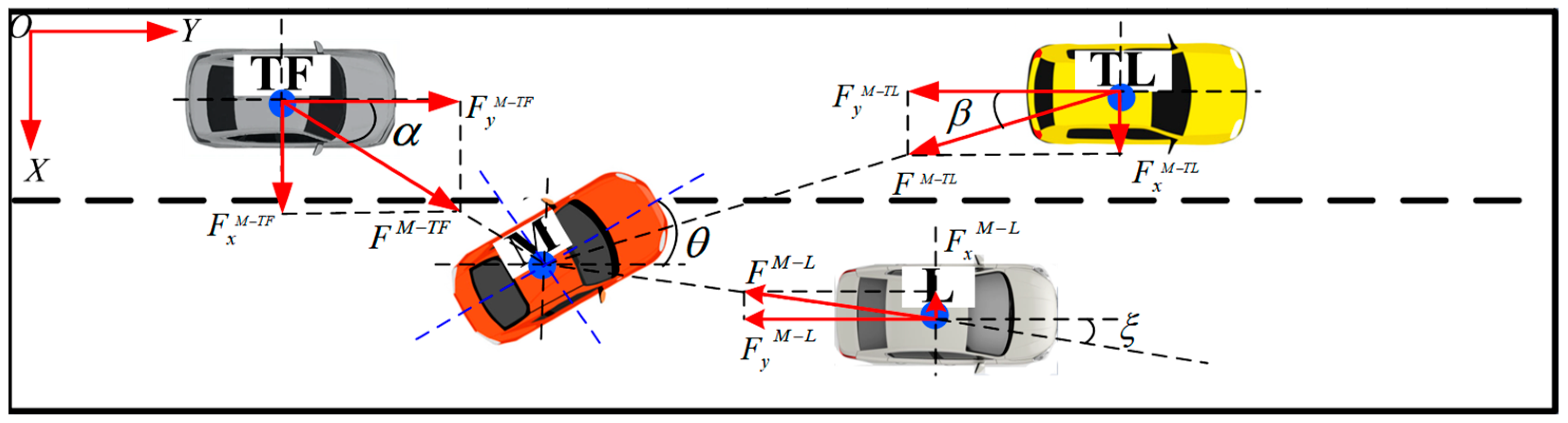
3.2.1. Acceptable Lane Changing Clearance between Vehicle M and Vehicle TL

There is a risk of collision between lane changing vehicle M and target lane leading vehicle TL in the process of lane changing, so it is necessary to study their interaction state. As shown in Figure 5, in order to avoid collision accidents between vehicle M and vehicle TL, the two vehicles should meet the conditions shown in the following formula, that is

$$G_a^{M-TL}\ge S_M-S_{TL}+G_{\min }+w\sin (\theta )$$

(6)

where, $G_a^{M-TL}$: the acceptable lane changing gap between vehicle M and vehicle TL; $S_M$: the distance of lane changing vehicle M after the end of lane changing; $S_{TL}$: the distance traveled by the leading vehicle TL in the target lane after the lane changing; $G_{\min }$: the longitudinal critical distance between the two vehicles at the end of the lane changing; $w$: the width of the lane changing vehicle; and $\theta$: the angle between the lane changing vehicle M and the horizontal direction of the road.

If a vehicle wants to implement lane changing in a network environment, it is necessary to calculate whether the acceptable gap of lane changing is satisfied on the premise of obtaining the operating parameters of surrounding vehicles, and the determination of $G_{\min }$ and $\Delta S$ is particularly critical. The following studies are conducted on $G_{\min }$ and $\Delta S$, respectively.

(1)

Longitudinal critical distance

The longitudinal critical distance indicates that the vehicle can safely follow the vehicle in front after completing the lane changing behavior under the premise of meeting this distance. Therefore, it can also be explained by the distance required for following. Shi Baiying [17] believes that the required safety distance is related to the speed and reaction time of the vehicle, and puts forward a formula:

$$G_{\min }=\eta v+\gamma v^2$$

(7)

where: $v$ represents the speed of the vehicle; $\eta$ indicates the response time of the vehicle; and $\gamma$ indicates the undetermined coefficients.

In the VTH following strategy [18], the required safety distance is related to the current vehicle speed and the speed difference between the front and rear vehicles, and the expression is as follows:

$$G_{\min }=(t_0-c_v\Delta v)v$$

(8)

where: $v$ represents the speed of the vehicle; $\Delta v$ represents the speed of the front car minus the speed of the rear car; and $t_0$ and $c_v$ are undetermined coefficients.

In the intelligent network environment, the acquisition, processing, and transmission of information have been improved qualitatively, the vehicle reaction time is basically negligible, and the driving state parameters between vehicles can be obtained in real time. Therefore, the setting of the longitudinal critical distance should also introduce the influence of the acceleration difference between the front and rear vehicles, and the expression is:

$$G_{\min }=(t_0-c_v\Delta v-c_a\Delta a)v$$

(9)

where: $\Delta a$ is the acceleration difference between the front and rear vehicles, $c_a$ is the undetermined coefficient, and other parameters are the same as above.

According to the above analysis, the longitudinal critical distance between vehicle M and vehicle TL can be obtained as:

$$G_{\min }=\left[t_0-c_v(v_{TL}-v_M)-c_a(a_M-a_{TL})\right]v_M$$

(10)

(2)

Safe critical time for lane changing

The safe critical time for lane changing represents the time it takes for lane changing vehicles and interacting vehicles to reach the same speed during lane changing. When the two cars reach the same speed, if there is no collision risk, there will be no collision later. In the actual lane changing process, the running state of the leading vehicle in the target lane is very little affected by the lane changing vehicle and can be ignored, so the state of vehicle TL generally does not change during the lane changing process. The initial lane changing speed and acceleration of vehicle M are set to be $v_M$ and $a_M$, respectively, and the initial speed and acceleration of vehicle TL are set to be $v_{TL}$ and $a_{TL}$, respectively. Based on the above assumptions, the safe critical time of vehicle M and vehicle TL under different moving states is plotted when $v_M<v_{TL}$, as shown in Figure 6. By analyzing the diagram, it can be found that if vehicle M completes the lane change under the condition of meeting the safe critical time of lane changing, the distance difference between the two vehicles with the same speed will no longer change. Therefore, the shaded part of the figure can be used to represent the distance difference between the two cars, which is $\Delta S=\frac{\left(v_M-v_{TL}\right)T}{2}$, and the safe critical time for lane changing satisfies the formula $T=\frac{v_{TL}-v_M}{a_M-a_{TL}}$, which is $\Delta S=-\frac{{\left(v_{TL}-v_M\right)}^2}{2\left(a_M-a_{TL}\right)}$.

Therefore, by synthesizing formulas (6) and (10), the expression of acceptable lane changing clearance between vehicle M and vehicle TL can be obtained as:

$$\left\{\begin{array}{c}{G}_a^{M-TL}\ge -\frac{{\left(v_{TL}-v_M\right)}^2}{2\left(a_M-a_{TL}\right)}+G_{m\mathrm{in}}+w\sin (\theta )\\ \\ G_{\min }=\left[t_0-c_v\left(v_{TL}-v_M\right)-c_a\left(a_{TL}-a_M\right)\right]v_M\end{array}\right.$$

(11)

3.2.2. Acceptable Lane Changing Clearance between Vehicle M and Vehicle TF

There is a risk of collision between lane changing vehicle M and target lane following vehicle TF in the process of lane changing, so it is necessary to study their interaction state. As shown in Figure 7, in order to avoid collision accidents between vehicle M and vehicle TF, the two vehicles should meet the conditions shown in the following,

$$G_a^{M-TF}\ge S_{TF}-S_M+G_{\min }+w\sin (\theta )$$

(12)

where, $G_a^{M-TF}$ represents the acceptable lane changing gap between vehicle M and vehicle TF; $S_M$ indicates the distance traveled by lane changing vehicle M after the end of lane changing; and $S_{TF}$ indicates the distance traveled by the target lane following car TF after the end of the lane changing.

Based on the above lane changing scenario assumption, the speed of vehicle TF is larger than that of vehicle M. In the early stage of lane changing, when the distance between the two vehicles is large enough, the vehicle TF can perform uniform or even accelerated motion. When the distance between the two vehicles is reduced, vehicle TF, as the following vehicle after the lane changing of vehicle M, belongs to the forced vehicle, and the vehicle will slow down under the influence of the repulsion force. It is assumed that the initial lane changing speed and acceleration of vehicle M are $v_M$ and $a_M$, respectively, and the initial speed and acceleration of vehicle TF are $v_{TF}$ and $a_{TF}$, respectively. Similarly, it is assumed that the lane changing is completed when the speed of the two vehicles is equal, and the distance difference does not change after that; setting $v_M<v_{TF}$ can obtain the safe critical time of vehicle M and vehicle TF under different moving states as $T=\frac{v_{TF}-v_M}{a_M-a_{TF}}$ and the distance difference between the two vehicles as $\Delta S=\frac{{\left(v_{TF}-v_M\right)}^2}{2\left(a_M-a_{TF}\right)}$.

In summary, the expression of acceptable lane changing clearance between vehicle M and vehicle TF can be obtained as

$$\left\{\begin{array}{c}{G}_a^{M-TF}\ge \frac{{\left(v_{TF}-v_M\right)}^2}{2\left(a_M-a_{TF}\right)}+G_{\min }+w\sin (\theta )\\ \\ G_{\min }=\left[t_0-c_v\left(v_M-v_{TF}\right)-c_a\left(a_M-a_{TF}\right)\right]v_{TF}\end{array}\right.$$

(13)

3.2.3. Acceptable Lane Changing Clearance between Vehicle M and Vehicle L

There is a collision risk between lane changing vehicle M and leading vehicle L in the lane changing process, so it is necessary to study their interaction state. As shown in Figure 8, in order to avoid angle collision between vehicle M and vehicle L, the two vehicles should meet the conditions as follows,

$$G_a^{M-L}\ge S_M-S_L+G_{\min }+w\sin (\theta )$$

(14)

where: $G_a^{M-L}$ represents the acceptable lane changing gap between vehicle M and vehicle TF; $S_M$ indicates the distance traveled by lane changing vehicle M after the end of lane changing; and $S_L$ indicates the distance traveled by the leading vehicle L in the current lane during the lane changing.

Since the motion state of the leading vehicle L in the current lane is basically not affected by the lane changing vehicle M, the leading vehicle L may perform uniform motion, accelerating motion, or decelerating motion. The initial lane changing speed and acceleration of vehicle M are set to be $v_M$ and $a_M$, respectively, and the initial lane changing speed and acceleration of vehicle TF are set to be $v_L$ and $a_L$, respectively. According to the generation mechanism of lane changing intention, it can be seen that vehicle M is subject to the repulsive force of the leading vehicle before it generates the lane changing intention, so this paper assumes that the initial lane changing speed relation is $v_M>v_L$.

In this lane changing scenario, the collision that very easily happens is angle collision, and the time for the two vehicles to present the illustrated state is defined as $t_j$, which is usually taken as 1.8~3 s according to experience. If there is no angle collision between the two vehicles at this time, there will be no further collision risk. In this case, we get a distance difference of $\Delta S=\left(v_M-v_L\right)t_j+\frac{a_M{t_j}^2}{2}$.

In summary, the expression of acceptable lane changing clearance between vehicle M and vehicle L can be obtained as

$$\left\{\begin{array}{c}{G}_a^{M-L}\ge \left(v_M-v_L\right)t_j+\frac{a_M{t_j}^2}{2}+G_{\min }+w\sin (\theta )\\ \\ G_{\min }=\left[t_0-c_v\left(v_L-v_M\right)-c_a\left(a_L-a_M\right)\right]v_M\end{array}\right.$$

(15)

3.3. Vehicle Interaction Potential Lane Change Model Considering Acceptable Lane Changing Clearance

The vehicle potential field force is a short-range repulsive force, which is used to prevent other vehicles from approaching to ensure safe driving. In general, the greater the vehicle potential, the stronger the potential field force. In the process of lane changing, vehicles are affected by multiple vehicle potentials, so it is necessary to determine the potential field force generated by each vehicle on the lane changing vehicle, and then judge whether the vehicle meets the conditions of safe lane changing. The lane changing diagram of vehicles as shown in Figure 9 is drawn, and the action potential of vehicle TL, vehicle TF, and vehicle L on lane changing vehicle M is analyzed respectively.

The resulting action potential of vehicle TL on vehicle M:

$$U^{M-TL}=\frac{\epsilon }{v-u}\left[u{\left(\frac{G_a^{M-TL}}{L_{M-TL}}\right)}^v-v{\left(\frac{G_a^{M-TL}}{L_{M-TL}}\right)}^u\right]·\exp \left(a_M\cos \left(\theta -\beta \right)\right)·\frac{d^{\ast }}{\left|d^{\ast }\right|}$$

(16)

To simplify the formula, let $\lambda =\exp \left(a_M\cos \left(\theta -\beta \right)\right)·\frac{d^{\ast }}{\left|d^{\ast }\right|}$, and the potential field force generated by vehicle TL on vehicle M:

$$F^{M-TL}=\frac{\lambda uv\epsilon }{v-u}\left[u\frac{{\left(G_a^{M-TL}\right)}^u}{L_{M-TL}^{u+1}}-v\frac{{\left(G_a^{M-TL}\right)}^v}{L_{M-TL}^{v+1}}\right]$$

(17)

With $\eta =\frac{\lambda uv\epsilon }{v-u}$, we get

$$F_x^{M-TL}=\eta \left[u\frac{{\left(G_a^{M-TL}\right)}^u}{L_{M-TL}^{u+1}}-v\frac{{\left(G_a^{M-TL}\right)}^v}{L_{M-TL}^{v+1}}\right]\sin \beta$$

(18)

$$F_y^{M-TL}=\eta \left[u\frac{{\left(G_a^{M-TL}\right)}^u}{L_{M-TL}^{u+1}}-v\frac{{\left(G_a^{M-TL}\right)}^v}{L_{M-TL}^{v+1}}\right]\cos \beta$$

(19)

where: ${F_x}^{M-TL}$ represents the potential field force generated by vehicle TL on vehicle M in the direction of $x$; ${F_y}^{M-TL}$ represents the potential field force generated by vehicle TL on vehicle M in direction $y$; and $\beta$ represents the angle between the centroid connection of vehicle TL and vehicle M and axis $y$.

Vehicle TF exerts force on vehicle M:

$$F^{M-TF}=\eta \left[u\frac{{\left(G_a^{M-TF}\right)}^u}{L_{M-TF}^{u+1}}-v\frac{{\left(G_a^{M-TF}\right)}^v}{L_{M-TF}^{v+1}}\right]$$

(20)

$${F_x}^{M-TF}=\eta \left[u\frac{{\left(G_a^{M-TF}\right)}^u}{L_{M-TF}^{u+1}}-v\frac{{\left(G_a^{M-TF}\right)}^v}{L_{M-TF}^{v+1}}\right]\sin \alpha$$

(21)

$${F_y}^{M-TF}=\eta \left[u\frac{{\left(G_a^{M-TF}\right)}^u}{L_{M-TF}^{u+1}}-v\frac{{\left(G_a^{M-TF}\right)}^v}{L_{M-TF}^{v+1}}\right]\cos \alpha$$

(22)

where: ${F_x}^{M-TF}$ represents the potential field force generated by vehicle TF on vehicle M in direction $x$; ${F_y}^{M-TF}$ represents the potential field force generated by vehicle TF on vehicle M in direction $y$; and $\alpha$ represents the angle between vehicle TF and vehicle M’s centroid connection and axis $y$.

In the same way, it can be analyzed that vehicle L exerts force on vehicle M:

$$F^{M-L}=\eta \left[u\frac{{\left(G_a^{M-L}\right)}^u}{L_{M-L}^{u+1}}-v\frac{{\left(G_a^{M-L}\right)}^v}{L_{M-L}^{v+1}}\right]$$

(23)

$${F_x}^{M-L}=\eta \left[u\frac{{\left(G_a^{M-L}\right)}^u}{L_{M-L}^{u+1}}-v\frac{{\left(G_a^{M-L}\right)}^v}{L_{M-L}^{v+1}}\right]\sin \xi$$

(24)

$${F_y}^{M-L}=\eta \left[u\frac{{\left(G_a^{M-L}\right)}^u}{L_{M-L}^{u+1}}-v\frac{{\left(G_a^{M-L}\right)}^v}{L_{M-L}^{v+1}}\right]\cos \xi$$

(25)

where: ${F_x}^{M-L}$ represents the potential field force generated by vehicle L on vehicle M in direction $x$; ${F_y}^{M-L}$ represents the potential field force generated by vehicle L on vehicle M in direction $y$; and $\xi$ represents the angle between vehicle L and vehicle M’s centroid connection and axis $y$.

According to the vehicle interaction potential theory, when the workshop distance is less than the acceptable gap, the force generated by the interaction potential is a repulsive force. When the workshop distance is greater than the acceptable gap, the result is gravitational force. However, combined with the actual driving of the vehicle, even if the longitudinal gravity of the rear vehicle TF on the lane changing vehicle M is generated, it cannot be characterized as attracting the rear acceleration of the vehicle M.

Therefore, on the basis of the coordinate system established in Figure 9, the vehicle interaction potential combined with the actual analysis of lane changing can be obtained:

(1)

When ${F_y}^{M-L}\ge 0$, vehicle M continues to follow.

(2)

When ${F_y}^{M-L}<0$, the vehicle is subjected to repulsive force resulting in lane changing intention. When ${F_y}^{M-TL}<0$ or ${F_y}^{M-TF}>0$ indicates that vehicle M is being repulsed longitudinally by vehicle TL or vehicle TF, lane changing is not recommended. When ${F_y}^{M-TL}\ge 0$ and ${F_y}^{M-TF}\le 0$, it means that vehicle TL and vehicle TF exert gravity on vehicle M and can change lanes. At this time, vehicle M is subjected to lateral gravity and is $\left|{F_x}^{M-TF}\right|+\left|{F_x}^{M-TL}\right|$, which causes vehicle M to accelerate crosswise and change lanes. As vehicle M turns to drive, vehicle L exerts a lateral repulsive force on vehicle M, forcing vehicle M to accelerate laterally away from the original lane, so the sum of lateral forces received by the vehicle is $\left|F_x\right|=\left|{F_x}^{M-L}\right|+\left|{F_x}^{M-TF}\right|+\left|{F_x}^{M-TL}\right|$. According to the relationship between force and acceleration, the following can be obtained: $\left|a_x\right|=\frac{\left|F_x\right|}{m}$, that is, vehicle M will accelerate to the target lane with an acceleration of $\left|a_x\right|$.

4. Model Verification

4.1. Numerical Simulation Analysis

Based on the above analysis of acceptable lane changing clearance, Python3.0 software was used for numerical simulation to analyze the change in acceptable lane changing clearance under different vehicle speeds and accelerations.

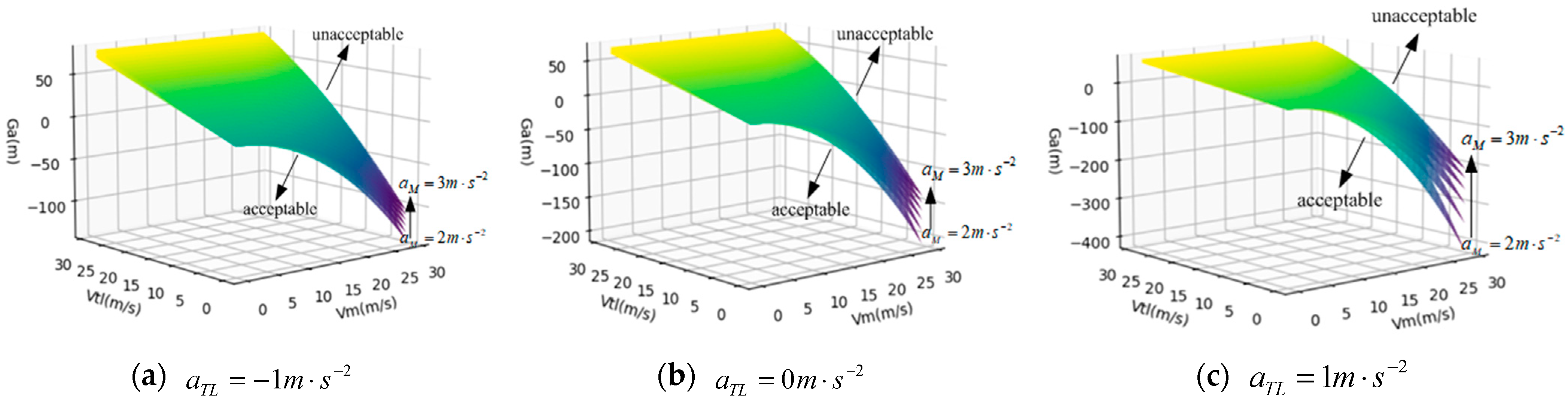
4.1.1. Simulation Analysis of Acceptable Clearance of Lane Changing between Vehicle M and Vehicle TL

The simulation of the acceptable clearance of vehicle M and vehicle TL for lane changing is carried out by establishing a space coordinate system with the speed of the two vehicles as the x and y axes and the acceptable clearance for lane changing as the z axis, and then output the relation surface between the speed of the two vehicles and the acceptable clearance for lane changing. The acceleration of the lane changing vehicle $a_M$ is set to the variation scale of $0.2 \mathrm{m}·{\mathrm{s}}^{-2}$ within the range of $2 \mathrm{m}·{\mathrm{s}}^{-2}~3 \mathrm{m}·{\mathrm{s}}^{-2}$. In reference [19], the parameters were calibrated as $t_0=1.5,c_v=0.05,c_a=0.3$, the length of $w=3.5$, and lane changing angle $\theta =3^{\circ }$, and the following parameter values are the same. Based on the assumption $v_M<v_{TL}$ above, the change in acceptable clearance between vehicle M and vehicle TL for lane changing in the case of acceleration of $a_{TL}=-1 \mathrm{m}·{\mathrm{s}}^{-2}$, $a_{TL}=0 \mathrm{m}·{\mathrm{s}}^{-2}$, $a_{TL}=1 \mathrm{m}·{\mathrm{s}}^{-2}$, and in the target lane is plotted, respectively, as shown in Figure 10.

It can be seen from the results that the acceptable lane changing clearance is determined by the speed and acceleration of vehicle M and vehicle TL. As the speed difference between vehicle TL and vehicle M increases, the acceptable lane changing clearance decreases. With the increase in vehicle M acceleration, the acceptable clearance of lane changing increases. With the increase in TL acceleration of the leading vehicle in the target lane, the acceptable lane changing clearance decreases. In the process of lane changing in the network environment, in order to meet the speed expectation of the lane changing vehicle, the vehicle TL is accelerated without slowing down to ensure the safety of lane changing.

4.1.2. Simulation Analysis of Acceptable Clearance of Lane Changing between Vehicle M and Vehicle TF

The simulation of the acceptable clearance of lane changing between vehicle M and vehicle TF is carried out, and the parameter settings are the same as above. Based on the above assumption $v_M<v_{TF}$, the change in acceptable lane clearance between vehicle M and vehicle TF when the target lane follows vehicle TF at the acceleration of $a_{TF}=-1 \mathrm{m}·{\mathrm{s}}^{-2}$, $a_{TF}=0 \mathrm{m}·{\mathrm{s}}^{-2}$, and $a_{TF}=1 \mathrm{m}·{\mathrm{s}}^{-2}$, respectively, is drawn, as shown in Figure 11.

It can be seen from the results that the acceptable clearance of lane changing is determined by the speed and acceleration of vehicle M and vehicle TF. As the speed difference between vehicle TF and vehicle M increases, the acceptable clearance of lane changing increases. With the increase in vehicle M acceleration, the acceptable clearance of lane changing decreases. With the increase in vehicle TF speed in the target lane, the acceptable clearance of lane changing increases. In the process of lane changing in a networked environment, in order to meet the expectations of lane changing vehicles, vehicle TF is slowed down to ensure lane changing safety when vehicle M is at a constant speed or accelerating.

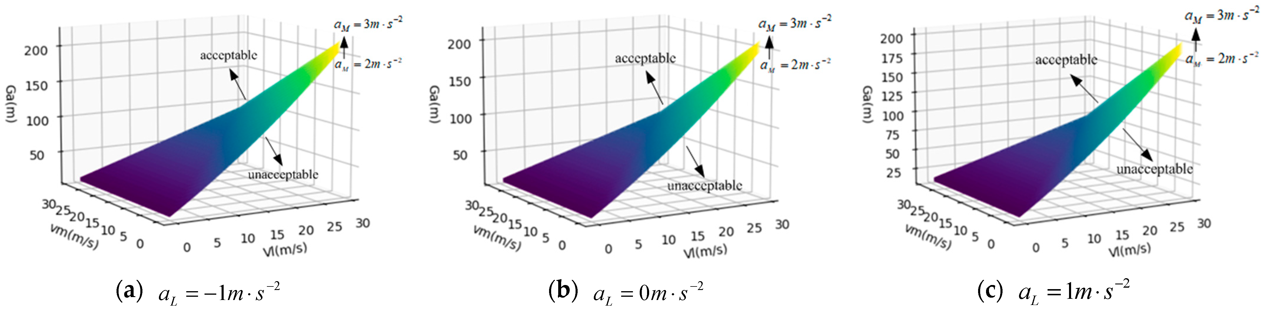
4.1.3. Simulation Analysis of Acceptable Clearance of Lane Changing between Vehicle M and Vehicle L

Simulation of acceptable clearance of lane changing of vehicle M and vehicle L are carried out, and the parameter settings are the same as above. Based on the above assumption $v_M>v_L$, the change in acceptable lane clearance between vehicle M and vehicle L when the acceleration of leading vehicle L is $a_L=-1 \mathrm{m}·{\mathrm{s}}^{-2}$, $a_L=0 \mathrm{m}·{\mathrm{s}}^{-2}$, and $a_L=1 \mathrm{m}·{\mathrm{s}}^{-2}$, respectively, is plotted, as shown in Figure 12.

It can be seen from the results that the acceptable clearance of lane changing is determined by the speed and acceleration of vehicle M and vehicle L. As the speed difference between vehicle M and vehicle L increases, the acceptable clearance of lane changing increases. As the speed of lane changing vehicle M increases, the acceptable clearance of lane changing increases. As the speed of the leading vehicle L increases, the acceptable clearance of lane changing decreases. In the process of lane changing in the network environment, in order to meet the speed expectation of the lane changing vehicle, vehicle M can ensure the safety of lane changing by accelerating with vehicle L under the condition of uniform speed.

To sum up, the acceptable clearance of vehicle lane changing is affected by different motion states of interacting vehicles, and the above simulation analysis shows that the acceptable clearance model established in this study is consistent with the actual lane changing state.

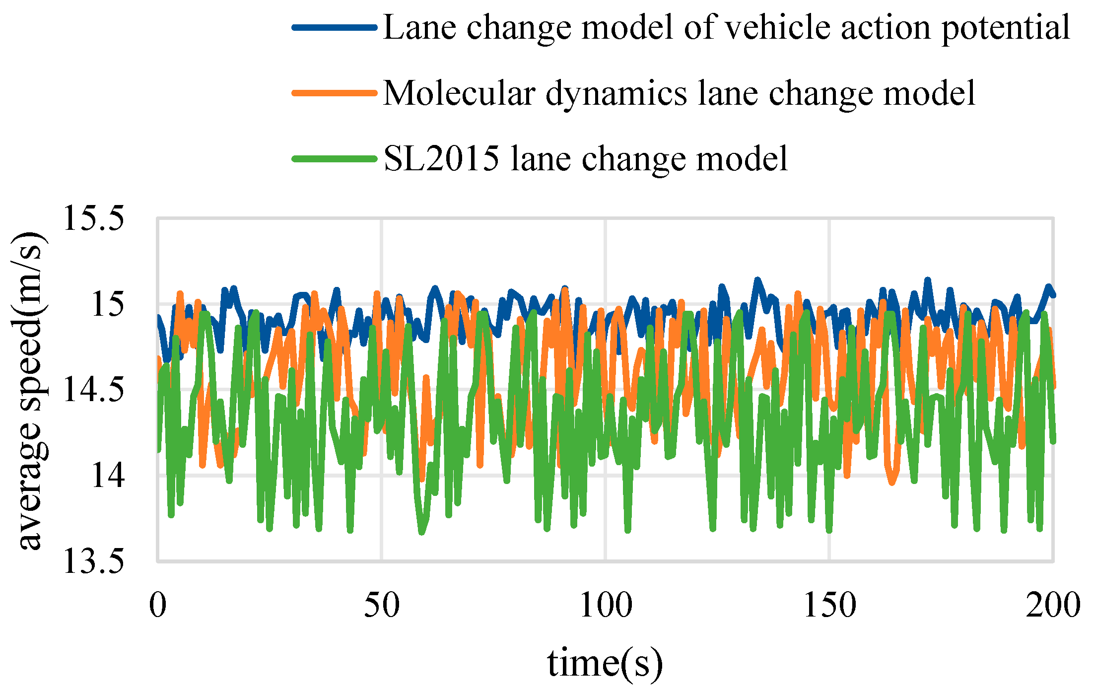
4.2. Model Evaluation

In order to verify that the vehicle interaction potential lane change model can effectively improve the speed of traffic flow and reduce the speed fluctuation of traffic flow, SUMO software (win64-1.11.0) was used to conduct simulation experiments. The experiment scene was set as a 2 km long one-way, three-lane road with a speed limit of 60 km/h. This was the simulation interface of the lane changing experiment, as shown in the Figure 13. After the vehicle generates the intention of lane changing, it will turn on the left turn signal to signal, which well reflects the environmental state of the lane changing vehicle in the model.

In reference to the calibration results of the vehicle action potential model parameters, the values $u=0.713$, $v=1.648$, $\gamma =0.032$, and $s_0=2.11$ are taken, and combined with the parameters determined in 4.1, so that the model is determined.

The traffic flow operating parameters output by the experiment were graphically analyzed, as shown in Figure 14, reflecting the changes of the average speed and average acceleration of the traffic flow. In the intelligent network environment, the vehicle can obtain the operating parameters of the surrounding vehicles in real time, and then judge the environment in which it is driving to achieve uninterrupted speed adjustment. Figure 14a reflects the change in the average speed of the traffic flow. It can be seen from the figure that the traffic flow on the whole is traveling at a relatively ideal speed, and the average speed fluctuates at $0.6 \mathrm{m}·{\mathrm{s}}^{-1}$, which is relatively gentle. Figure 14b reflects the average acceleration of traffic flow. It can be seen from the figure that the overall average acceleration is distributed within the range of $-0.7 \mathrm{m}·{\mathrm{s}}^{-2}~0.7 \mathrm{m}·{\mathrm{s}}^{-2}$, and the acceleration state is obviously more than the deceleration state, which is also the reason why the average speed of traffic flow is relatively ideal.

In order to better verify the effectiveness of the vehicle action potential lane changing model, a set of comparison experiments between the vehicle action potential lane changing model, molecular dynamics lane changing model, and SL2015 lane changing model are designed. Among them, SL2015 is a built-in model in SUMO software, which can well simulate the lane changing behavior of vehicles. The molecular dynamics lane changing model is based on the Lennard-Jones 6–12 potential function. The vehicle action potential proposed in this study is modified on the basis of the Lennard-Jones molecular interaction potential, and the comparison of the three parameters has a certain significance.

Figure 15 shows the average output speed of the three models when the traffic flow is roughly stable. It can be seen that compared with the molecular dynamics lane changing model and SL2015 lane changing model, the average traffic flow speed of the vehicle action potential lane changing model is greatly improved, the average speed fluctuation is relatively gentle, and the driving comfort of the vehicle is higher.

5. Conclusions

(1)

The establishment of vehicle interaction potential based on Lennard-Jones potential introduced the correction of vehicle shape, speed, acceleration, and steering angle, which made up for the previous research on the molecular lane changing model directly based on the Lennard-Jones 6-12 potential function that ignored the huge differences between particles and vehicles in parameters such as mass and velocity. By drawing the spatial distribution map of the vehicle action potential field under different motion states, the changes in the vehicle action potential field with vehicle speed, acceleration, and steering angle can be directly analyzed, which makes the study of vehicle microscopic behavior based on molecular dynamics more realistic.

(2)

In the previous study of the molecular dynamics lane changing model, the setting of longitudinal critical distance after lane changing only considered the speed and acceleration of the current vehicle, ignoring the influence of the running state of the leading vehicle on the critical safety distance after lane changing. In this paper, the acceleration of the front vehicle is introduced into the longitudinal critical distance, and the relationship between the acceptable clearance of lane changing and the speed difference and acceleration difference of the interacting vehicle is clarified through the analysis of the safe critical time of lane changing. The acceptable gap expressions between lane changing vehicle M and leading vehicle L and target lane leading vehicle TL and target lane following vehicle TF were constructed, respectively. Through simulation analysis of different motion states of interactive vehicles, reasonable suggestions were put forward for lane changing behavior in the networked environment.

(3)

A lane changing model based on vehicle interaction potential is established, the action potential and potential field force generated by the surrounding interacting vehicles of the lane changing vehicle are analyzed, and the driving decision of vehicle M under different potential field forces is given. Compared with the molecular dynamicsbased lane changing model and LS2015 model, the effectiveness of the proposed method is verified. It has theoretical guiding significance for vehicle lane changing behavior decisions in future intelligent network environments.

(4)

The following problems should be considered in the following research: First, the paper compares the vehicle as a molecule. In order to simplify the model, the center of mass of the vehicle is taken as the coordinate point, and the influence of the vehicle shape on the distance is ignored. Second, the end of the paper uses simulation tests to verify the analysis, not using the data of natural experiments to verify, and there may be more uncertain factors in the actual driving environment; in following research, still needed is the use of data of natural experiments to verify the effectiveness.

References

1. Gipps, P.G. A Model for the Structure of lane changing Decisions. Transp. Res. Part B 1986, 20, 403–414. [Google Scholar] [CrossRef]
2. Olsen, E.C.; Lee, S.E.; Wierwille, W.W.; Goodman, M.J. Analysis of distribution, frequency, and duration of naturalistic lane changings. Proc. Hum. Factors Econ. Soc. 2002, 46, 740–741. [Google Scholar]
3. Ahmed, K.I. Modeling Drivers’ Acceleration and Lane Changing Behavior. Ph. D. Thesis, Massachusetts Institute of Technology, Cambridge, MA, USA, 1999. [Google Scholar]
4. Jia, H.F.; Tan, Y.L.; Li, Q.; Yang, D. Gap Acceptance Model Construction in Expressway Junction Area considering Driver Characteristics. J. Jilin Univ. (Eng. Technol. Ed.) 2015, 45, 55–61. [Google Scholar]
5. Xu, L.H.; Ni, Y.P.; Luo, Q.; Huang, Y.G. Lane-changing model based on minimum safety distance. J. Guang Xi Norm. Univ. 2011, 12, 1–6. [Google Scholar]
6. Wang, C.L.; Li, Z.L.; Chen, Y.Z.; Dai, G.P. Reach on lane-change models considering restricted space. J. Highw. Transp. Res. Dev. 2012, 1, 121–127. [Google Scholar]
7. Shang, L.; Lu, H.P. Model of vehicle behavior under multi-lane road conditions. J. Hua Zhong Univ. Sci. Technol. (Nat. Sci. Ed.) 2007, 35, 115–117. [Google Scholar]
8. Khatib, O. Real-time obstacle avoidance for manipulators and mobile robots. In Proceedings of the IEEE International Conference on Robotics and Automation, St. Louis, MO, USA, 25–28 March 1985; pp. 500–505. [Google Scholar]
9. Gao, K.; Yan, D.; Yang, F.; Xie, J.; Liu, L.; Du, R.; Xiong, N. Conditional artificial potential field-based autonomous vehicle safety control with interference of lane changing in mixed traffic scenario. Sensors 2019, 19, 4199. [Google Scholar] [CrossRef] [PubMed]
10. Wolf, M.T.; Burdick, J.W. Artificial Potential Functions for Highway Driving with Collision Avoidance. In Proceedings of the IEEE International Conference on Robotics and Automation, Pasadena, CA, USA, 19–23 May 2008; pp. 3731–3736. [Google Scholar]
11. Li, L.H.; Gan, J.; Qu, X.; Ran, B. Vehicle lane changing model based on safety potential field theory in intelligent network environment. China J. Highw. Transp. 2021, 34, 184–195. [Google Scholar]
12. Bham, G.H. Estimating driver mandatory lane change behavior on amulti-ane freeway. In Proceedings of the 88th Annual Meeting of the Transportation Research Board, Washington, DC, USA, 11–15 January 2009; Transportation Research Board: Washington, DC, USA, 2009. [Google Scholar]
13. Yang, M.M.; Wang, X.S.; Quddus, M. Examining lane change gap acceptance, duration and impact using naturalistic driving data. Transp. Res. Part C Emerg. Technol. 2019, 104, 317–331. [Google Scholar] [CrossRef]
14. E, W.J. Research on Vehicle-Vehicle Conflict Detection and Resolution Algorithm at Unsignalized Intersection; Jilin University: Changchun, China, 2012. [Google Scholar]
15. Li, J. Study on Traffic Flow Characteristics and Its Model Based on Molecular Dynamics; School of Automobile and Transportation of Qingdao University of Technology: Qingdao, China, 2018. [Google Scholar]
16. Qu, D.Y.; Zhang, K.K.; Wang, T.; Song, H.; Dai, S.-c. Analysis of lane changing decision Behavior and Molecular Dynamics Modeling of Autonomous vehicle. J. Jilin Univ. (Eng. Ed.) 2024, 700–710. [Google Scholar]
17. Shi, B.Y.; Yang, X.G.; Yu, X.F. Modeling and simulation of discretionary lane-change considering the combination with the car-following model. J. Transp. Sci. Eng. 2009, 25, 91–96. [Google Scholar]
18. Yanakiev, D.; Kanellakopoulos, I. Non linear spacing policies for automated heavy-duly vehicles. IEEE Trans. Veh. Technol. 1998, 47, 1365–1377. [Google Scholar] [CrossRef]
19. Jia, Y.F.; Qu, D.Y.; Zhao, Z.X.; Wang, T.; Song, H. Car-following Decision-making and Model for Connected and Autonomous Vehicles Based on Safety Potential Field. Transp. Syst. Eng. Inf. 2022, 22, 85–97. [Google Scholar]
Figure 1. Schematic diagram of initial stationary vehicle potential field.
Applsci 14 04659 g001
Figure 2. Road environment diagram.
Applsci 14 04659 g002
Figure 3. Distribution diagram of vehicle potential field under different motion states.
Applsci 14 04659 g003aApplsci 14 04659 g003b
Figure 4. Lane changing scene setting.
Applsci 14 04659 g004
Figure 5. Lane changing process between vehicle M and vehicle TL.
Applsci 14 04659 g005
Figure 6. Safe critical time of lane changing under different motion states.
Applsci 14 04659 g006
Figure 7. Lane changing process between vehicle M and vehicle TF.
Applsci 14 04659 g007
Figure 8. Lane changing process of vehicle M and vehicle L.
Applsci 14 04659 g008
Figure 9. Force analysis of lane changing vehicle M.
Applsci 14 04659 g009
Figure 10. Acceptable lane changing clearance between vehicle M and vehicle TL.
Applsci 14 04659 g010
Figure 11. Acceptable lane changing clearance between vehicle M and vehicle TF.
Applsci 14 04659 g011
Figure 12. Acceptable lane changing clearance between vehicle M and vehicle L.
Applsci 14 04659 g012
Figure 13. Simulation interface of lane changing experiment.
Applsci 14 04659 g013
Figure 14. Experimental data of vehicle action potential lane changing model.
Applsci 14 04659 g014
Figure 15. Comparison of average speeds of different models.
Applsci 14 04659 g015
Disclaimer/Publisher’s Note: The statements, opinions and data contained in all publications are solely those of the individual author(s) and contributor(s) and not of MDPI and/or the editor(s). MDPI and/or the editor(s) disclaim responsibility for any injury to people or property resulting from any ideas, methods, instructions or products referred to in the content.