Fatigue Damage Assessment of Turbine Runner Blades Considering Sediment Wear

Abstract

The wear phenomenon that occurs on the blades during operation has a significant impact on the fatigue life of the blades. To address the issue of fatigue life assessment for turbine runner blades subjected to increased dynamic stress due to sediment wear, taking a specific high-head hydropower unit’s mixed-flow turbine as the research subject, a hydraulic model of the turbine was established. The wear zones of the runner blades are determined based on the distribution of the flow field’s velocity and the sediment volume fraction. According to the wear rate formula for runner blade material, the amount of wear on the blades is determined, and the dynamic stress data for the dangerous areas of the blades under different degrees of wear are calculated using a unidirectional fluid–structure coupling method. The load spectrum of the time–stress history data for the dangerous area at different levels of wear was compiled using the rain-flow counting statistical method. The operating time ratios for the flood season and the non-flood season are combined. Based on the fatigue cumulative damage theory, the total fatigue damage at the maximum stress part of the runner blade was calculated for different stages of wear, providing a reference for the life calculation of mixed-flow hydraulic turbines.

1. Introduction

As a renewable energy, hydropower is one of the pillars of China’s electric power system, playing a crucial role in promoting economic development. As the core component of a hydropower station, the turbine’s safety, stability, and reliability are paramount. In Southwest China, rivers feature substantial water flow, significant head variation, and high sediment content, which varies greatly with the seasons. This variability leads to severe wear on the turbine’s internal structures and diminishes the fatigue strength of the runner blades. The causes of fatigue damage to the turbine’s runner components are also complex. Ensuring the stable operation of hydropower units thus requires a detailed estimation of the fatigue damage and life of the turbine runner components.

Unterluggauer et al. [1] proposed a numerical method to understand critical operational areas and access fatigue damage, and compared the simulation results with measured data. The appropriate consistency between the measured data and simulation results indicates that the numerical simulation method is feasible for calculating fatigue damage in hydraulic turbines. Chen et al. [2] compared the stress distribution and deformation of pump blades under positive and reverse power generation conditions. Theoretical and numerical calculations of fatigue strength were conducted, and a preliminary estimation of the runner’s fatigue life was made to investigate how to extend the service life of the pump station. Zhu et al. [3] employed bidirectional fluid–structure coupling analysis on a Francis turbine to determine its stress characteristics, iteratively solving for the coupling coefficients in both fluid and structural equations until convergence. Based on the structural analysis, the maximum stress, maximum displacement, and wear locations within the turbine were identified, providing valuable insights for the design and optimization of the turbine. Zhang [4] employed the finite element method to analyze the stress and strain of a turbine blade and calculated the blade’s stress fatigue characteristics using specialized fatigue analysis software. The results of the analysis were in line with actual requirements and offered valuable data for the analysis of fatigue characteristics in turbine blades. Wang et al. [5] conducted internal flow field analysis to determine the blade surface pressure under various startup conditions of a hydropower station’s Francis turbine, and established the blade stress distribution for analyzing the turbine’s fatigue performance. They also optimized the design of the blade’s critical areas to enhance the blade’s fatigue life. Zhang [6] performed a numerical simulation analysis on the hydrodynamic performance and structural characteristics of a hydraulic turbine using two-way fluid–structure coupling calculations. The analysis considered the effects of turbine speed and water depth variations and predicted the fatigue life of the blades. The accuracy of these computational results was validated through model testing. ALSTOM Company [7,8] used numerical simulation to analyze the pressure pulsations and equivalent stresses of the runner blades in a low-head Francis turbine, and, combining this with measured stresses, predicted the fatigue life of the runner under various operating conditions. Ghomashchi R. [9] analyzed the bucket blades of the Francis turbine and determined that fatigue failure of the runner blade was due to repeated alternating or cyclic stress, which, despite being lower than the normal yield strength, occurred over a long period. Han et al. [10] conducted fatigue life prediction research on the rotating blade of a generator set. The blade’s stress was determined through transient dynamic analysis of the blade surface load. The blade’s life was calculated using both the linear Miner criterion and a fuzzy life estimation method, and the results of the two methods were compared. It was determined that the fuzzy life estimation method proved more accurate for calculating blade life. Zhu [11] studied fatigue life prediction methods and crack growth mechanism models for mechanical structural components, based on a multi-factorial modified fatigue theory. Bayesian theory was introduced for data fusion during experimental data processing, aiming to achieve high-precision predictions of structural fatigue life and reliability assessments. Zhao et al. [12,13,14,15] took a high-head Francis turbine as the research subject, analyzing and calculating the pressure pulsations and equivalent stresses on the surface flow fields of both long and short blades under various operating conditions using numerical simulation. They also studied the primary factors influencing the fatigue life of the turbine runner. Applying the theory of fatigue cumulative damage, the fatigue life of runner blades under different working conditions was determined. Gao et al. [16] took the runner of a hydropower station as an example and considered factors affecting the runner, including the average stress, stress concentration, surface state, and size factor. They used MSC Fatigue software to calculate the runner’s life, providing valuable data for the subsequent operation and maintenance of the power station. To ensure the safe operation of the Zhang pumped storage power station, Huang et al. [17] conducted unsteady numerical analysis of the full flow field and predicted the fatigue life of the runner under various operating conditions based on the dynamic stress characteristics of the runner. Zhao et al. [18] used fluid–structure coupling calculations to analyze the characteristics of the internal flow field in a specific type of hydraulic turbine, studied the causes of the runner’s vibration, and predicted the fatigue life of the runner under fluctuating water pressure. Heng et al. [19] aimed to explore the impact of vibration under complex operating conditions on the fatigue reliability life of turbine blades in a hydraulic turbine. They established different reliability models for various operating conditions and developed an integrated reliability assessment model based on these models. The correctness and feasibility of the integrated reliability assessment model were also verified.

In summary, numerical analysis and calculation of the internal flow field and fluid–structure coupling of the runner are relatively mature at present. Most studies on the fatigue life of runner blades focus on analyzing the surface dynamic stress of the blades under specific operating conditions to directly predict the life of the blades, without considering the impact of structural changes caused by wear on the blades during operation on their service life. However, blade wear occurs in practice, altering the structure of the affected areas and resulting in increased dynamic stress, which significantly impacts the blade’s fatigue life. Therefore, it is essential to consider blade wear in actual operation when predicting the life of runner blades. This paper analyzes the stress changes in the critical areas of the hydraulic turbine runner blade before and after wear occurs, and determines the progression of fatigue damage in these areas under continuous wear. Ultimately, it is concluded that considering the wear of the blades is essential for estimating the service life of the turbine runner, which more accurately reflects the actual operational lifespan. It provides insights for the safe and stable operation and maintenance of the turbine unit in the future.

2. Establishment of a Computational Model for Hydraulic Turbines

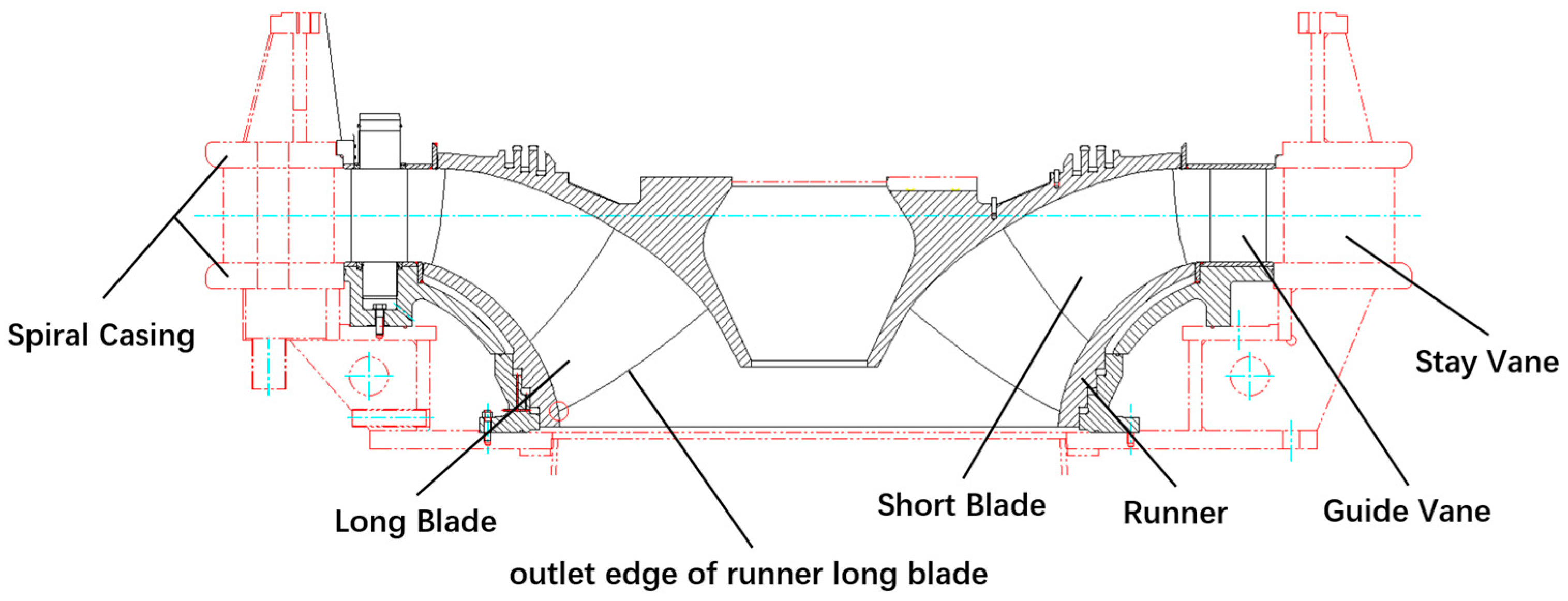
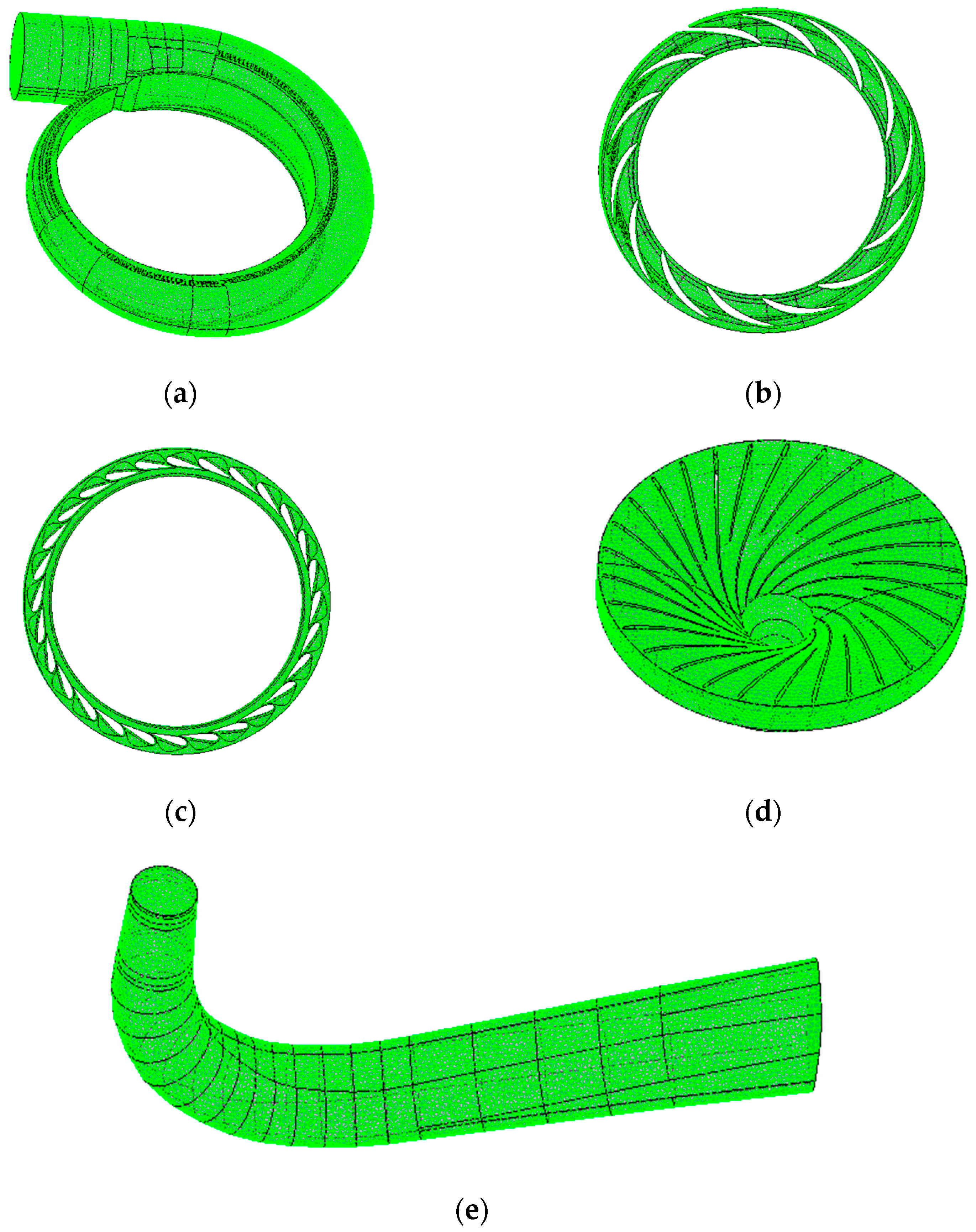
2.1. Establishment and Mesh Division of a Hydraulic Model of a Hydro Turbine

In this paper, the Francis turbine of a high-head hydropower unit was taken as the research object, and the establishment of a geometric model is the basis of simulation work. The sectional view of the high-head turbine is shown in Figure 1. The model parameters are shown in

Table 1. Basic parameters of hydraulic turbine.

Name	Units	Parameter
Mass flow rate	m3/s	16
Rated speed	Rad/min	500
Waterhead	m	282
Runner diameter	m	2.35
Guide vane height	m	2.88
Fixed guide vane	Unit	14
Movable guide vane	Unit	28
Long blade	Unit	15
Short blade	Unit	15

. The runner diameter is 2.35 m, the distribution circle diameter of guide vane is 2.65 m, the guide vane height is 2.88 m, and the head is 282 m; there are 14 fixed guide vanes, 28 movable guide vanes, 15 long blades and 15 short blades of the runner, and the rated speed is 500 rad/min. Each component needs to be assembled after 3D modeling separately.

The hydraulic model of the Francis turbine consists of five parts: volute, fixed guide vane, movable guide vane, runner, and drainpipe. This paper utilizes 3D modeling software to conduct geometric modeling of the entire flow path of the hydraulic turbine, and ICEM software is used to mesh the computational fluid dynamics domains of various internal flow components of the hydraulic turbine. Because each component is associated with a distinct flow field, it is essential to model and divide each component separately, as shown in Figure 2. The turbine runner flow domain is a significant rotating region, and to ensure the precision of the computational outcomes, it is necessary to augment the mesh density within this domain. Additionally, other fluid domains feature irregular geometric shapes at the arc transitions, which also demand high-quality meshing. To enhance calculation accuracy with limited computing resources, an unstructured grid is utilized.

2.2. Boundary Condition

In numerical simulation calculation, the setting of boundary conditions directly affects the accuracy of the calculation results. Therefore, the correct setting of boundary conditions is particularly important. In this paper, based on the actual working conditions of a power station, some parameters can be determined: the actual sediment content at the inlet of the hydropower station in annual flood season is 1.93 kg/m³ (volume fraction ϕ = 0.00074), and the median sediment diameter d = 0.02 mm. The average particle size of the sediment is used as the sand diameter. The inlet boundary condition is set as the flow velocity, and the outlet boundary condition is set as the pressure. The wall condition is set as a no-slip, fixed wall, and the standard wall function method is utilized in the region near the wall. The turbine’s runner is designated as the rotating domain, with the rotating domain’s speed set to 500 RPM. The remaining components are assigned to the static domain. The stationary domains are interconnected using a general connection, while the connections between the rotating and stationary domains are made using the Frozen Rotor Stator method for steady-state calculations and the Transient Rotor Stator method for transient cases. In the calculation of the transient flow field, the time step is set to 0.002 s. This interval corresponds to the time taken for the runner to rotate through 6 degrees. The convergence criterion is set to an accuracy of 1 × 10⁻⁶. The total duration of the calculation is 1.2 s, which equates to 30 cycles.

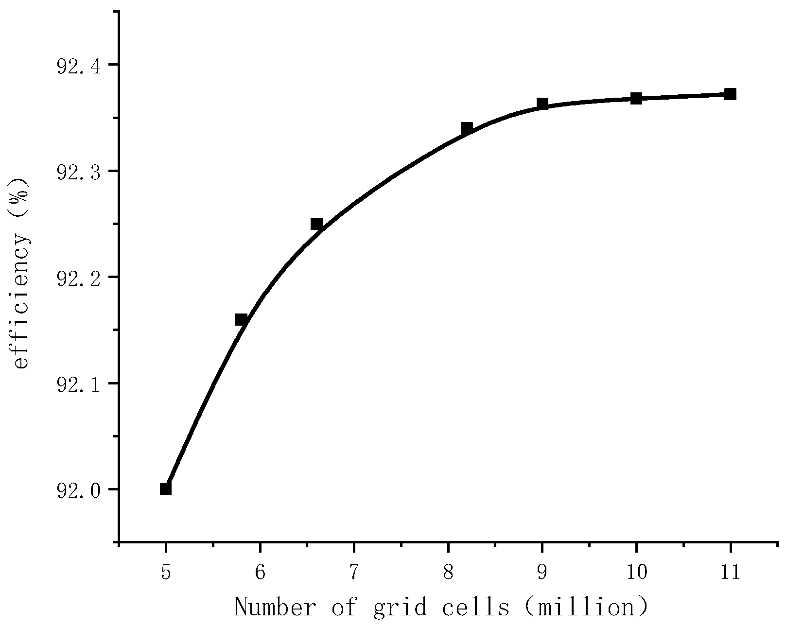
2.3. Check for Grid Independence

The accuracy and time cost of the numerical calculation are determined by the quality and quantity of the grid. Once the number of grids reaches a certain level, accuracy will not improve significantly further, but the time required for calculation increases greatly. Therefore, it is necessary to test the grid independence of the turbine flow components, divide the turbine full flow channel calculation model into several groups with different grid numbers, and then calculate the unit efficiency of the turbine full flow channel calculation model with different grid numbers.

It can be seen in Figure 3 that when the number of grids is less than 8.5 million, the unit efficiency increases as the number of grids increases. When the number of grids is greater than 9 million, the efficiency change of the unit tends to be flat as the number of grids increases. Therefore, considering the constraints of limited computing resources, the number of grids is determined to be 9.02 million to ensure the accuracy of the calculations. The grid quality of each fluid component is shown in

Table 2. Fluid mesh quality of various components.

Mesh Cell	Spiral Casing	Guide Vane	Stay Vane	Runner	Draft Tube
Mesh quantity (million)	1.78	1.45	1.34	2.7	1.74
Quality	0.48	0.52	0.5	0.47	0.55

. The grid quality value of each flow component is greater than 0.2, so the grid quality meets the requirements.

3. Numerical Calculation of Dynamic Stress on the Runner Blades of a Turbine

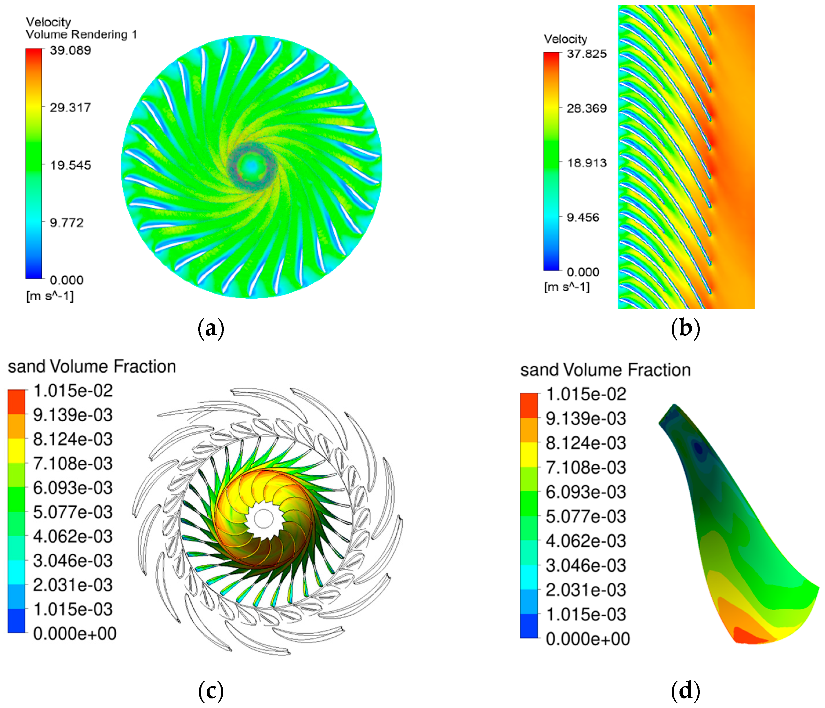
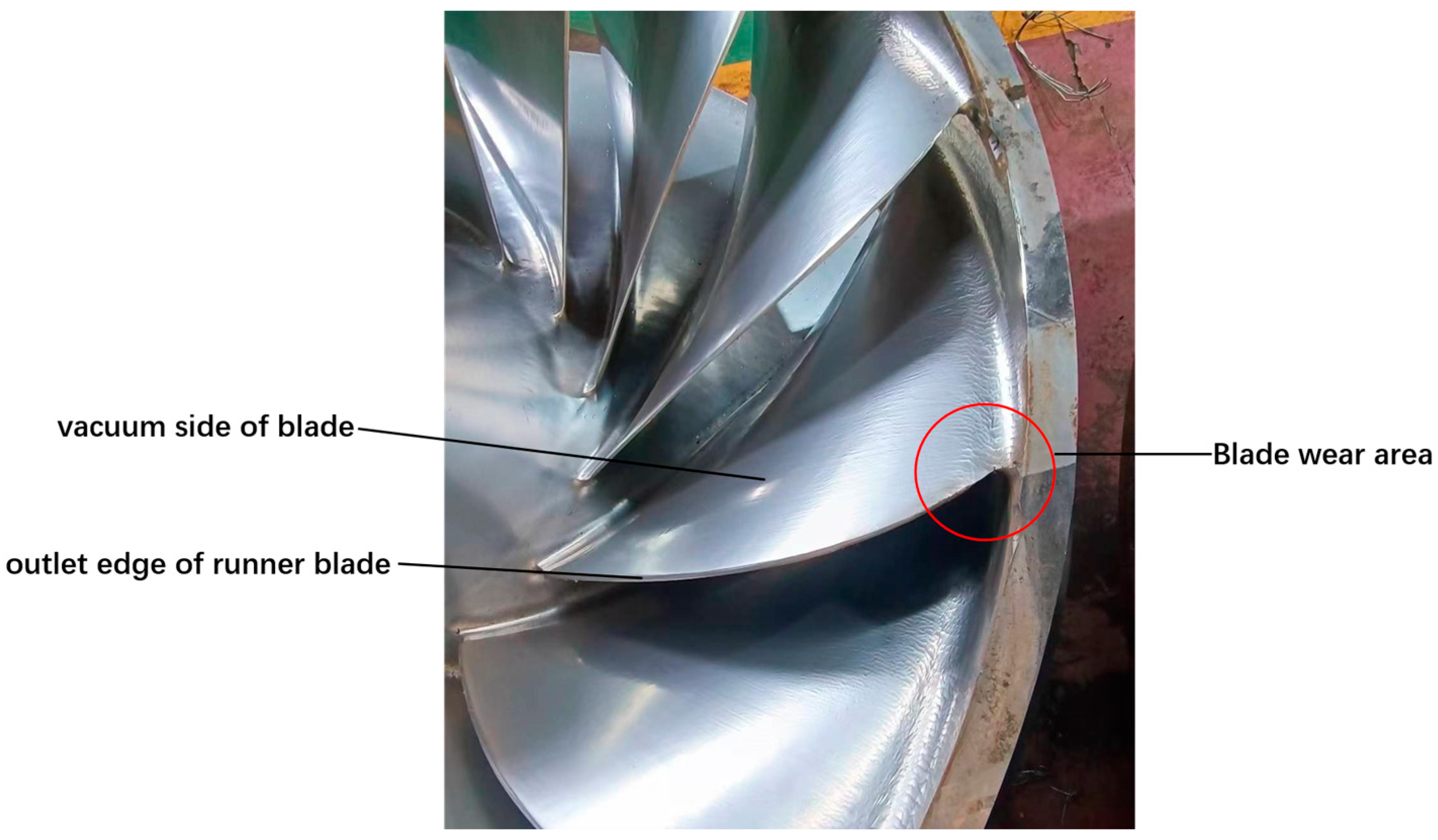
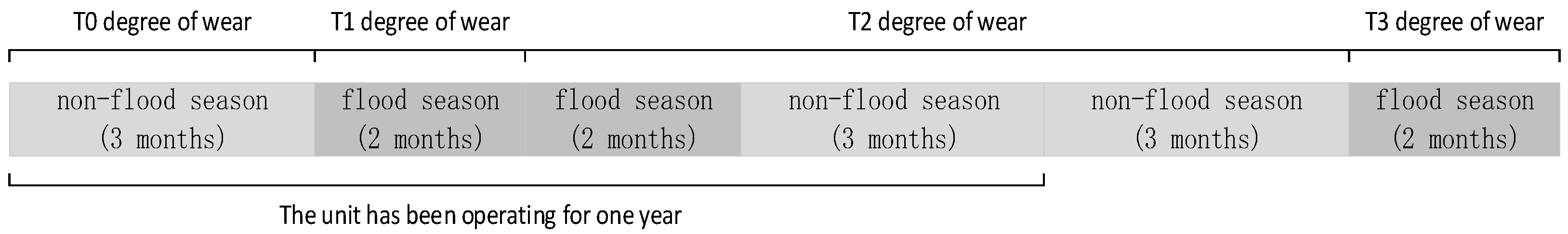
3.1. Identification of Wear Locations and Quantification of Wear on Turbine Runner Blades

According to the normal working conditions, the numerical simulation of the internal flow field of the turbine was carried out. By analyzing the flow characteristics of the fluid inside the turbine runner, the flow velocity distribution and sediment concentration distribution results of the internal flow field of the turbine runner were obtained. Based on these results, the wear area inside the turbine runner was determined. It can be seen in Figure 4 that the water flow passes through the inside of the runner, and the flow velocity first decreases and then increases from the entrance to the exit of the runner. The closer to the lower ring, the higher the flow velocity at the corresponding position. In addition, the fluid velocity around the long blade increases as it gets closer to the outlet of the runner, and the overall flow velocity on the back of the blade is greater than that on the working surface of the blade; especially when the back of the blade is near the water edge at the tail, the velocity reaches the maximum. Therefore, wear is more likely to occur at the back of the blade near the water edge than at other parts of the runner. Analyzing the sediment volume fraction distribution on the runner blade surface reveals that the sediment content is higher on the back of the blade near the lower ring compared to other areas. The degree of wear on the runner blade is influenced by the flow velocity of sand and the sediment concentration. Following the velocity distribution pattern of the flow field on the blade surface, it is evident that the area with the highest sediment flow velocity and concentration is on the back of the blade near the lower ring. Consequently, it can be deduced that the most severe wear occurs on the back of the blade near the lower ring, with the wear degree increasing as it approaches the water edge of the runner.

Figure 5 shows a runner that has been in service for some time. It can be seen intuitively that the worn area of the runner blade is at the water edge, with the most severe wear occurring at the junction between the blade’s water edge and the runner’s lower ring. This observation aligns with the wear positions and trends predicted by the numerical analysis of the runner’s internal flow field.

After identifying the worn areas on the runner blade, the next step is to measure the extent of wear at these locations. This is followed by establishing a general formula to calculate the wear rate for the turbine’s flow components [20]:

$$E=K\cdot k_s\cdot S^M\cdot W^N$$

(1)

Here, K represents the influence coefficient for material properties and a comprehensive influence coefficient for other factors. k_s denotes the influence coefficient of sediment characteristics. S stands for sediment concentration, M represents an index, W indicates the relative water flow velocity, and N is the index.

Ensure that the sediment content is consistent with the actual hydropower station. Therefore, the influence coefficient k_s = 1.0, the sediment concentration index M = 1.0, and the sediment concentration about S = 1.93 kg/m³ were determined to obtain the relationship between the material wear amount of the runner blade and time [21].

$$\Delta H=0.65\times {10}^{-9}S\cdot W^{3.7}\cdot T$$

(2)

Considering the actual operating conditions of hydropower turbines, the wear on runner blades predominantly occurs during the flood season, a period that typically spans approximately four months, from May to September annually. The extent of wear on the blades is assessed by examining the flow field velocity near the water edge of the upper runner blade’s working surface and applying the wear rate formula specific to the blade material. Wear initially occurs on the back of the blade near the water edge, and as working time increases, this wear surface progressively thins. Once the wear reaches a certain degree, the material at the tail of the blade near the water edge is worn away. This advanced wear leads to structural changes in the blade’s tail. By calculating the water flow velocity on the surface of the wear area after the blade has experienced different degrees of wear, it was found that the variation in water flow velocity is relatively small. Therefore, in this paper, the water flow velocity is taken as a constant value when calculating the wear amount of the blade, with the velocity magnitude set at 37.82 m/s.

In this paper, the flow velocity at the worn area of the runner blade’s tail and the material wear rate formula were combined to determine the blade’s wear amount under various working times. The results are presented in

Table 3. Blade wear data.

Degree of Wear	T0	T1	T2	T3	T4	T5
Time (month)	0	2	4	6	8	10
Wear amount (mm)	0	1.1225	2.245	3.367	4.490	5.612

.

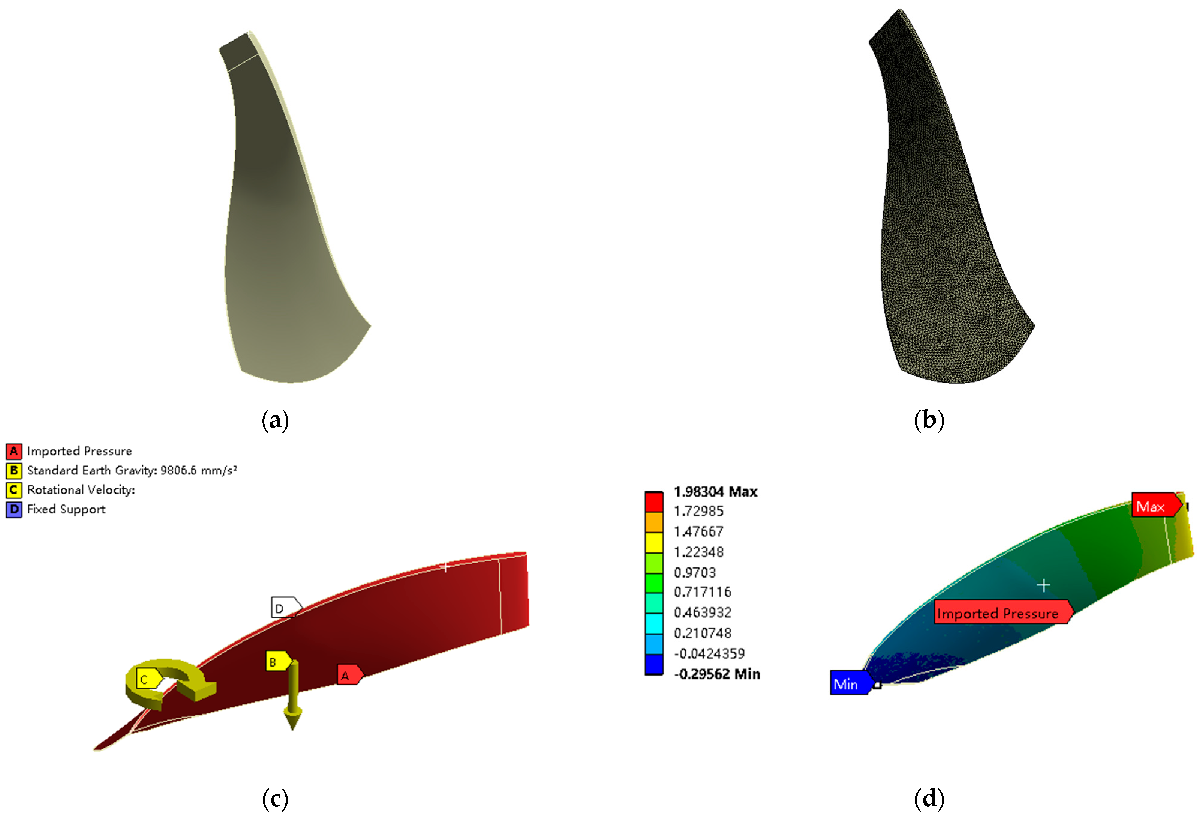
3.2. Establishment of a Fluid–Structure Interaction Model for Runner Blades and Setting of Boundary Conditions

Before conducting fluid–structure interaction analyses, 3D models of runner blades with varying degrees of wear are created using 3D modeling software. To ensure the accuracy of these analyses, it is essential that the blade models, regardless of their wear degree, are meshed to a high quality. The steps for modeling and meshing blades with different wear degrees are consistent. This section will provide a detailed introduction to the model of a blade at the wear degree T₀. Figure 6 displays the finite element model for a blade at wear degree T₀, which consists of 211,344 mesh elements and 386,134 nodes.

In this paper, the calculation of fluid–structure interaction for the runner blade employs a one-way coupling method, necessitating only the transfer of dynamic pressures from the fluid to the blade surface. The fluid domain and solid domain data transfer method used in this study is the Conservative interpolation method in ANSYS’s MFX multi-physics solver. When the fluid–structure interaction surface is perfectly matched, precise data transfer between the interfaces can be achieved. For this study, the interface between the fluid dynamics and finite element analysis modules facilitates the transmission of these dynamic pressure data. Prior to the transfer of dynamic stress data, the material for the runner blade must be specified, along with defining the material’s elastic modulus, Poisson’s ratio, density, and other relevant performance parameters. The runner blade is connected to the upper crown and lower ring of the runner via welding. To replicate the stress on the runner blade under actual operating conditions, constraints and fixed supports are applied to the interface between the runner blade and the upper crown and lower ring, as per the internal structural features of the runner. The runner operates at a rotational speed of 500 rad/min.

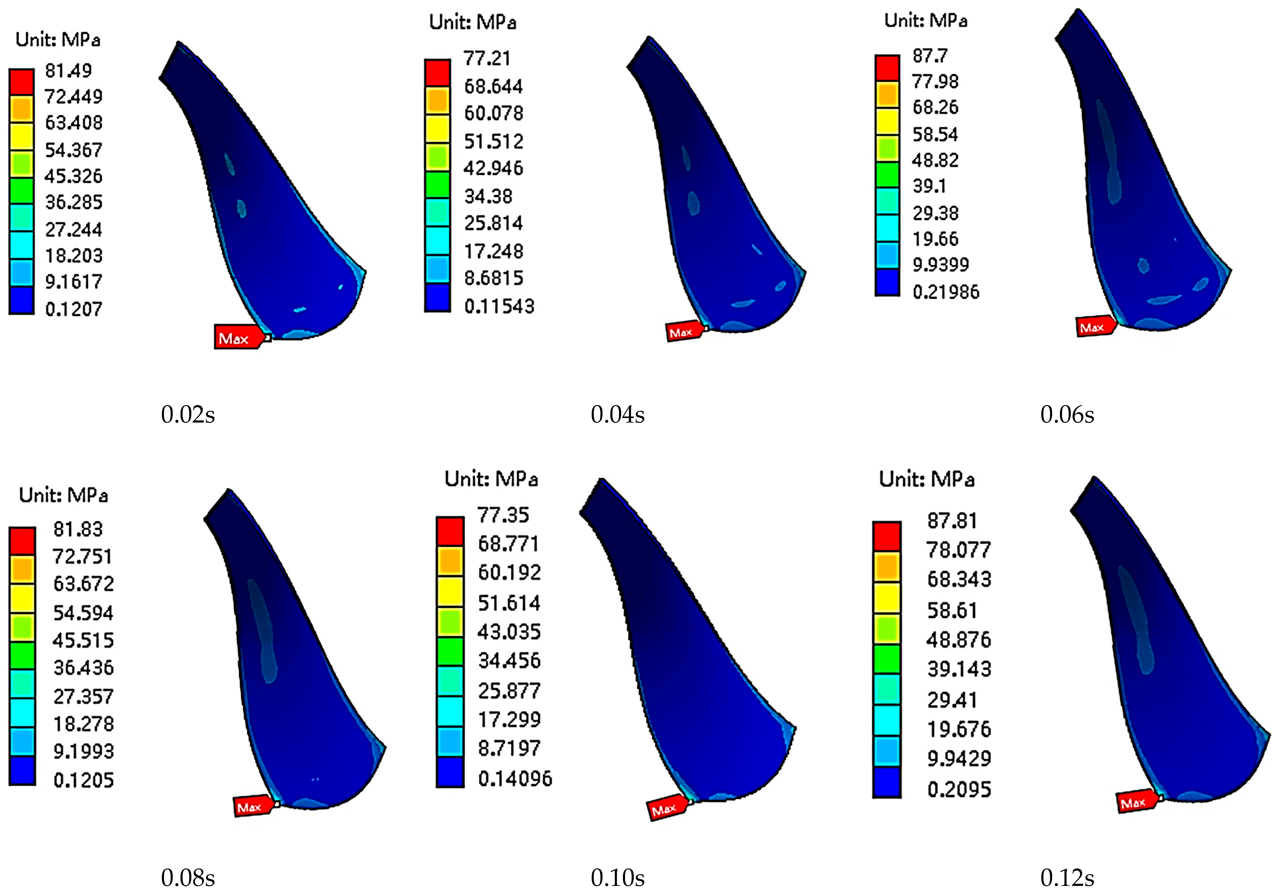
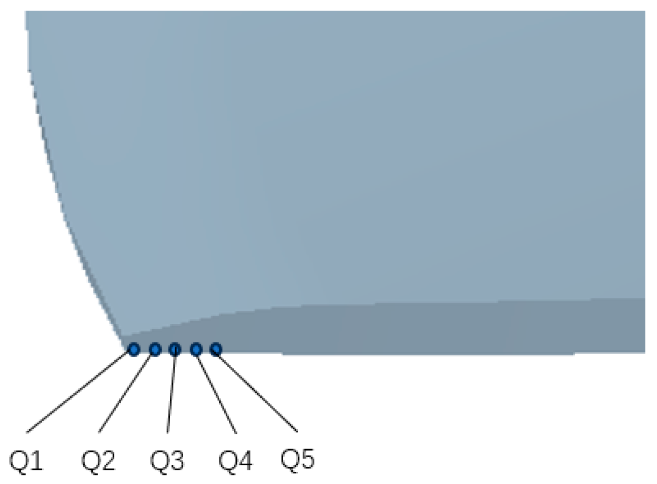
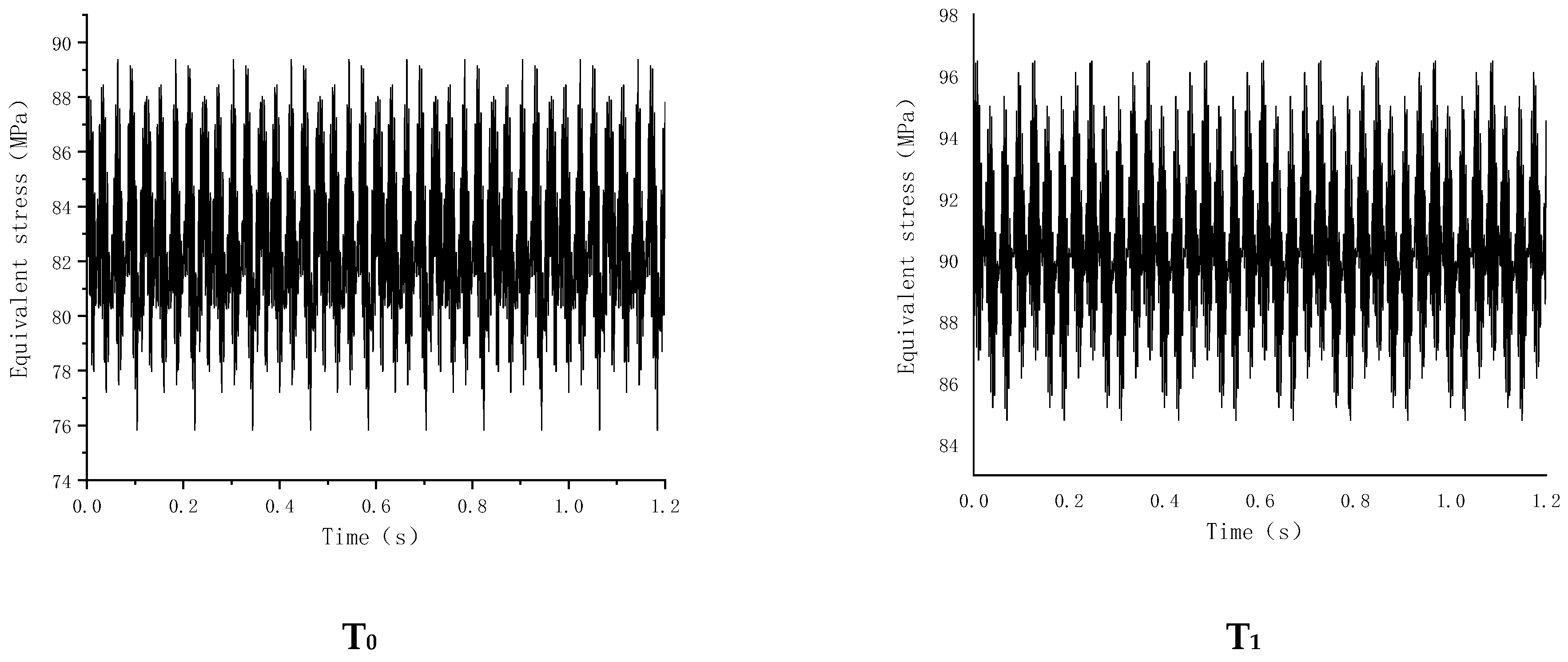
3.3. Dynamic Numerical Calculation of Runner Blades

Utilizing the fluctuating water pressure load data on the blade surface at various time points, derived from the transient flow field calculation of a Francis turbine’s entire passage, a transient dynamic stress mechanical analysis of the blade is performed. This analysis employs a unidirectional fluid–structure coupling method to couple the blade surface, yielding the equivalent stress–time history data on the blade surface at different times for various degrees of wear. Figure 7 presents the equivalent stress cloud diagrams of the blade at various instances throughout the rotation cycle, under the wear condition denoted as T₀.

It can be seen from the equivalent stress cloud diagram of the blade in the next rotation cycle under the wear degree of T₀ that the stress in the middle area of the blade is relatively small at different rotation times, and the stress is mostly concentrated in the area near the upper crown and the area near the lower ring at the water edge of the blade. With the rotation of the runner blade, the maximum stress area of the runner blade is always located in the area near the lower ring of the blade at the water exit edge, and the maximum stress in the area near the lower ring of the blade at different rotation times has obvious changes and fluctuations; this is caused by the alternating stress of the runner blade, and is also the primary reason for the crack and fatigue damage of the runner blade. Since the stress value and the amplitude of stress fluctuation in this region are the maximum values compared with other parts of the blade, the fatigue failure will be preferentially generated in this region, which is the dangerous part of the runner blade.

To thoroughly understand the variation in equivalent stress within the critical areas of the runner blade, stress monitoring points were established along the worn portion of the blade’s tail at locations of maximum stress for each degree of wear. These points are designated as Q₁, Q₂, Q₃, Q₄, and Q₅. The positioning of the stress probes is illustrated in Figure 8. Dynamic stress data for each monitoring point over a complete cycle and across various degrees of wear were extracted and are presented in

Table 4. Equivalent stress data of monitoring points on blades at different wear degrees in a single rotation cycle.

Time	Equivalent Stress at Monitoring Point Q1 (MPa)
	T0	T1	T2	T3	T4	T5
0.02	81.49	91.11	—	—	—	—
0.04	77.21	85.21	—	—	—	—
0.06	87.70	93.52	—	—	—	—
0.08	81.83	90.38	—	—	—	—
0.10	77.35	86.16	—	—	—	—
0.12	87.81	94.53	—	—	—	—
Time	Equivalent stress at monitoring point Q2 (MPa)
	T0	T1	T2	T3	T4	T5
0.02	71.42	80.75	94.48	—	—	—
0.04	68.50	77.96	89.00	—	—	—
0.06	81.55	87.24	99.87	—	—	—
0.08	72.67	82.73	94.80	—	—	—
0.10	70.81	79.26	89.07	—	—	—
0.12	81.86	86.85	100.1	—	—	—
Time	Equivalent stress at monitoring point Q3 (MPa)
	T0	T1	T2	T3	T4	T5
0.02	66.59	75.30	86.52	101.50	—	—
0.04	60.28	71.30	83.21	95.86	—	—
0.06	76.75	84.85	90.88	105.85	—	—
0.08	63.09	80.22	87.69	100.77	—	—
0.10	65.85	71.53	79.26	96.88	—	—
0.12	76.91	85.22	93.74	106.91	—	—
Time	Equivalent stress at monitoring point Q4 (MPa)
	T0	T1	T2	T3	T4	T5
0.02	59.50	62.52	79.50	90.24	113.27	—
0.04	53.81	66.77	77.38	87.20	105.08	—
0.06	72.50	80.97	87.67	104.08	119.48	—
0.08	60.83	62.03	83.08	95.96	113.05	—
0.10	61.44	65.75	78.91	89.9	102.16	—
0.12	71.71	81.21	87.03	103.17	118.44	—
Time	Equivalent stress at monitoring point Q5 (MPa)
	T0	T1	T2	T3	T4	T5
0.02	53.56	58.41	71.58	84.41	97.32	119.78
0.04	49.30	52.33	65.28	77.03	91.45	108.99
0.06	71.48	75.45	81.75	91.47	99.19	127.55
0.08	54.62	51.62	68.09	78.91	97.56	120.16
0.10	60.80	51.79	70.84	83.77	91.33	109.28
0.12	69.64	74.88	81.90	91.66	99.81	127.99

.

With the increase in wear time, the monitoring point will be worn out with the increase in wear amount. By extracting and analyzing the equivalent stress data of different wear times before the wear-out of each monitoring point, the specific data are shown in Table 4. It can be seen in the table that when the runner blade wear amount reaches T₂, the monitoring point Q₁ will be worn out. Therefore, only the stress–time history data under two blade wear degrees at T₀ and T₁ are available at the Q₁ position. When the blade wear amount reaches T₃, the monitoring point Q₂ will be worn out, so the monitoring point only has the stress–time history under the blade wear amount from T₀ to T₂. In a similar way, when the blade wear reaches T₅, the monitoring point Q₄ is worn out, and the monitoring point Q₅ still exists at this time. Therefore, the monitoring point Q₅ has all the stress–time history of the blade wear from T₀ to T_5.

Analysis of the equivalent stress data from blade monitoring points across various wear degrees in a single rotation cycle reveals a gradual decrease in stress from points Q₁ to Q₅ under identical wear conditions. This trend is attributed to the proximity of the monitoring point Q₁ to the blade’s water edge, where the blade experiences the highest alternating stress. The equivalent stress diminishes progressively with increasing distance from the water edge, from Q₁ to Q₅. Additionally, the stress levels at a given monitoring point exhibit a rising trend with greater wear amounts. Continuous wear on the blade will eventually lead to the degradation of the monitoring point closest to the water edge, causing an overall increase in stress levels at the remaining undamaged monitoring points.

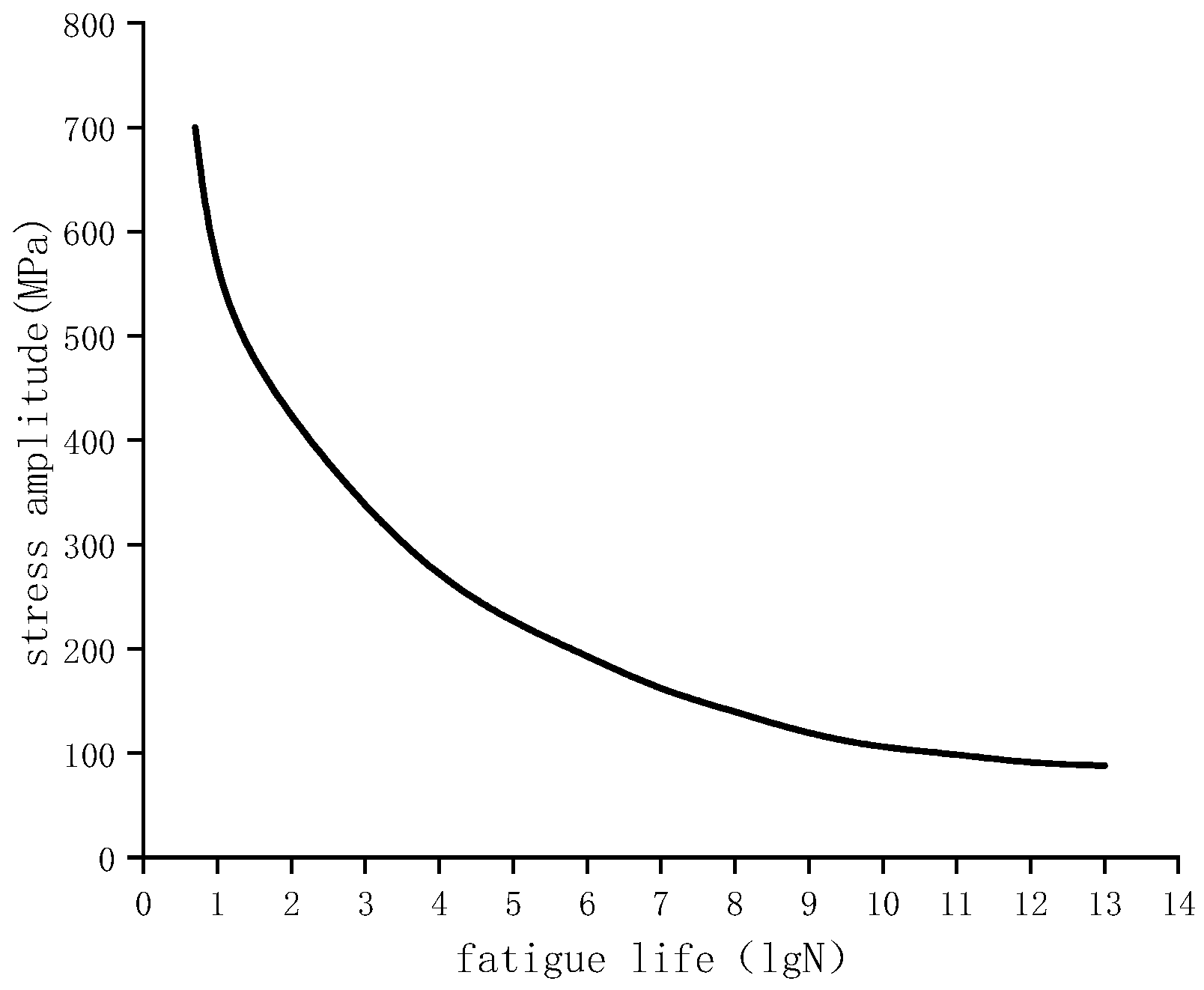
4. Fatigue Damage Assessment of Turbine Runner Blades

The von Mises equivalent stress–time history data for each monitoring point on the runner blade, under various degrees of wear, were extracted for a period of 1.2 s. Figure 9 illustrates the stress–time history at monitoring point Q₁ for the same duration under wear degrees T₀ and T₁.

As the stress–time history data from blade monitoring points at various wear times, derived from transient dynamics calculations, do not exhibit cyclic symmetry and are thus unsuitable for direct calculation of runner blade fatigue damage, this paper employs the rain-flow counting method to construct a load spectrum from the stress–time history data corresponding to different degrees of wear. This paper classifies the compiled stress amplitude data obtained under various degrees of wear and counts the number of cycles associated with each stress amplitude. Since the statistical stress amplitude is not directly applicable for calculating the fatigue damage of the runner blade across different wear degrees, it requires correction. The material chosen for the turbine runner in this study is ZG0Cr13Ni5MO. Its yield strength is 495 MPa, and the tensile strength is 735 MPa. The corrected stress amplitude is then compared with the fatigue life curve (S-N curve) of this material [22], as seen in Figure 10. With this comparison, the fatigue cycles for blade monitoring points under different stress amplitudes and two levels of wear can be directly ascertained. Since the wear on runner blades predominantly occurs during the flood season, this study adopts a time scale of 2 months between different wear levels of the blades. Given that the rotation cycle of the runner is 0.12 s, it is possible to determine the total number of cycles and the fatigue damage at each stress amplitude for the blade’s monitoring points under various wear conditions through a proportional relationship. Subsequently, the cumulative damage theory was applied to calculate the overall fatigue damage to the blade across different wear conditions, with the findings presented in

Table 5. The total fatigue damage of Q₁ point of blade running for 2 months under different wear degrees.

T0			T1
Stress Cycle Amplitude (MPa)	Amplitude of Correction (MPa)	Total Damage	Stress Cycle Amplitude (MPa)	Amplitude of Correction (MPa)	Total Damage
2.64	57.64	0.00670	0.28	61.15	0.01583
4.73	60.37		3.256	64.12
7.12	62.76		6.32	67.19
9.16	64.80		9.23	70.10
11.54	67.18		11.68	72.55

.

The total fatigue damage to the runner blade encompasses the damage accrued under both non-flood and flood season conditions. The unit operates for approximately 300 days annually, with the annual operational time history of the turbine depicted in Figure 11 for both the non-flood and flood seasons.

Combined with the running time under the working conditions in flood season and non-flood season, the total fatigue damage of the monitoring points from Q₁ to Q₅ before being worn off can be calculated, and the calculation results are as follows.

Therefore, the total fatigue damage of monitoring points Q₁ to Q₅ can be calculated before they are worn out. shown in

Table 6. The total fatigue damage of each monitoring point under different blade wear degrees.

Monitoring Point	Fatigue Damage under Different Blade Wear Degrees
	T0	T1	T2	T3	T4	T5
Q1	0.00670	0.01583	—	—	—	—
Q2	0.00463	0.00613	0.01724	—	—	—
Q3	0.00454	0.01052	0.01562	0.02921	—	—
Q4	0.00405	0.00459	0.01316	0.0169	0.0386	—
Q5	0.00246	0.00368	0.00498	0.01305	0.02774	0.04471

. According to the fatigue linear cumulative damage theory, when the cumulative total damage reaches the limit, the value of D equals 1, indicating that the material or part has sustained fatigue damage. Observing the fatigue damage values of each monitoring point reveals that as the wear amount increases, the fatigue damage at each point also increases gradually. A comparison of the total fatigue damage data between Q₃ and Q₄ shows a consistent pattern: both points are subject to wear due to the internal flow field before fatigue damage to the blade material occurs. In order to compare the changes in the fatigue damage of the runner blades with and without considering wear after working for the same time, the fatigue damage of the runner blades without considering wear at different working times is calculated, respectively. The total fatigue damage of blade danger points at different wear times considering runner blade wear is also compared, as shown in

Table 7. Total fatigue damage with and without blade wear at the same time.

Time (Year)	0	0.5	0.7	1.5	1.7	2.5
Irrespective of blade wear Fatigue damage	0	0.01675	0.02345	0.05025	0.05695	0.08375
Consider blade wear Fatigue damage	0	0.02588	0.03032	0.10902	0.11880	0.19601
Damage growth rate	0	0.54	0.29	1.17	1.09	1.34

.

From the table comparison, it is evident that considering blade wear results in a higher total fatigue damage than when wear is not considered. Additionally, the damage growth rate at the blade’s maximum stress point shows an increasing trend with wear. To better understand and compare these changes, a curve illustrating the pressure fatigue damage over time, with and without accounting for wear, was plotted, as seen in Figure 12.

The fatigue variation curves in Figure 11 reveal that fatigue damage to the blade, when wear is not considered, rises slowly with the runtime of the runner and is unaffected by the flood season conditions. Conversely, when wear is considered, the fatigue damage increases significantly with operation time. Notably, the fatigue damage accumulates gradually under non-flood conditions, but it increases markedly during the flood season. This significant increase is attributed to the structural changes caused by blade wear during the flood season, which in turn leads to a substantial rise in fatigue damage.

When considering wear, the runner blade is considered to have experienced fatigue failure when the maximum amount of fatigue damage is equal to 1. At this point, the life of the runner blade is determined to be approximately 8 years, which aligns with the actual service life of hydro turbines.

Therefore, the total fatigue damage at critical points, when accounting for blade wear, is significantly greater than when wear is not considered, which significantly affects the calculation of the blade’s fatigue life. Consequently, in basins with high sediment content, the effect of sediment on blade wear should be factored into the fatigue life calculations for hydraulic turbine runners.

5. Conclusions

This paper takes a mixed-flow hydraulic turbine from a high-head hydropower station as the research subject and investigates the changes in the fatigue life of the turbine runner caused by blade wear during actual operation. The main conclusions are as follows:

• As the turbine blades continuously wear, there is no significant change in the maximum pressure at the runner inlet, while the negative pressure at the outlet significantly increases. By analyzing the pressure fluctuations on the working and worn surfaces of the blade wear areas, it was found that as wear increases, the pressure fluctuations at the blade tail gradually strengthen, the negative pressure on the worn surface of the blades gradually decreases, and the pressure on the working surface slowly increases. Therefore, as the amount of blade wear increases, it can lead to unstable flow and cavitation near the outlet edge of the blades, which in turn affects the energy conversion efficiency of the runner and reduces the fatigue life of the blades.
• At different stages of blade wear, the maximum stress is always located at the connection area between the blade outlet edge and the lower ring, and the gradient of equivalent stress variation at this position is quite significant, with stress concentration effects also being quite pronounced. Therefore, fatigue damage tends to initiate preferentially in this area, which is entirely consistent with the actual sites of fatigue damage on turbine blades. Moreover, as the blades continue to wear, the overall stress level in the danger zone keeps increasing.
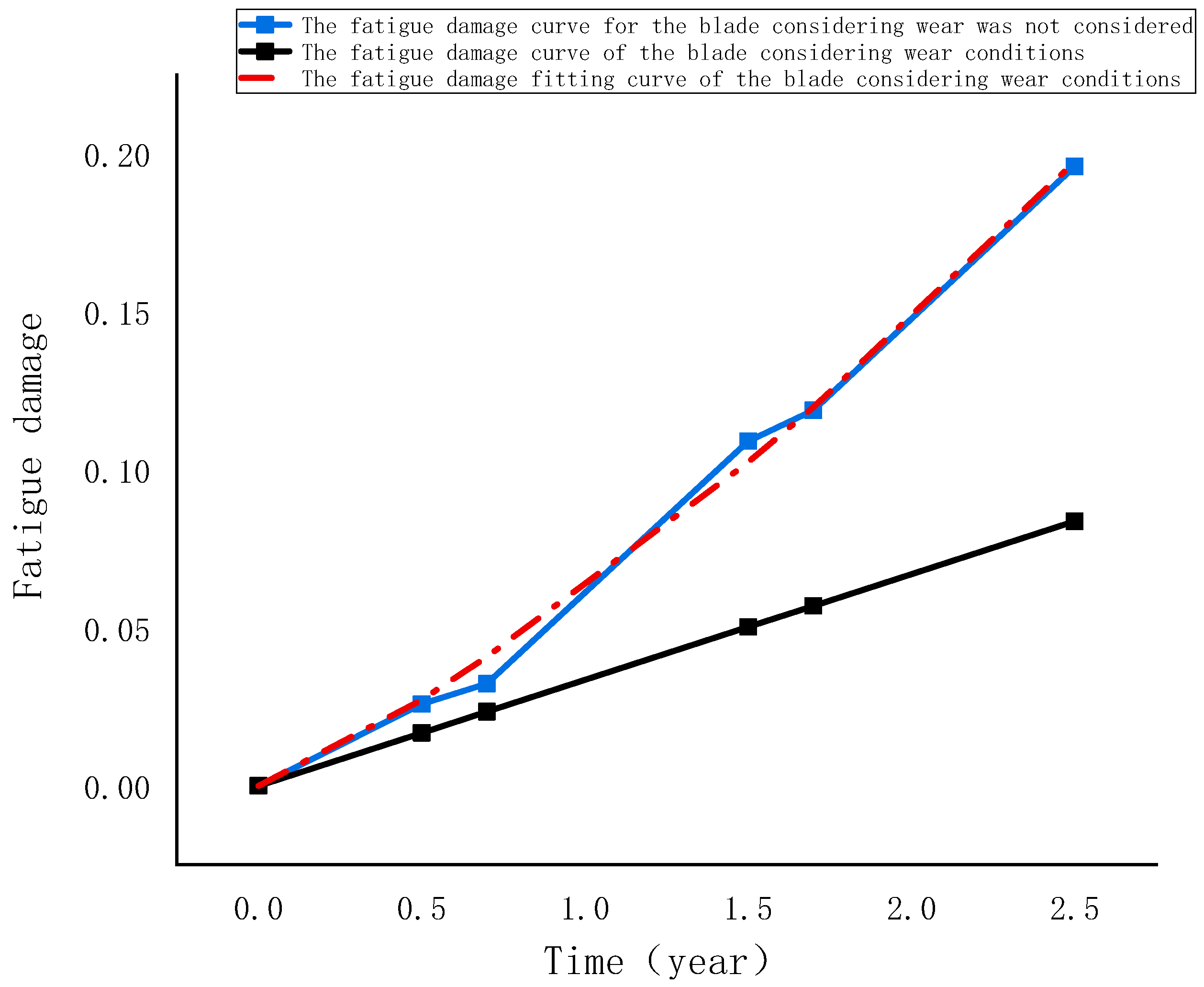
• As the blades continuously wear down, the fatigue damage in the critical areas of the blades increases progressively before they are worn away. The total fatigue damage at the danger points, when considering blade wear, shows a significant increase compared to the fatigue damage at the danger points without considering wear. This has a substantial impact on the calculation of the blade’s fatigue life. Therefore, in basins with high sediment content, the calculation of the fatigue life for hydraulic turbine runners should take into account the effects of sediment wear on the blades.

Through the research presented in this paper, the pattern of fatigue damage progression over operating time for a mixed-flow hydraulic turbine, considering wear, has been established. Calculations indicate that the fatigue life of the hydraulic turbine, when wear is taken into account, is approximately 8 years, which aligns with practical conditions. This provides valuable insights for the safe and reliable operation and maintenance of hydraulic turbine units in the future.

References

1. Unterluggauer, J.; Doujak, E.; Bauer, C. Numerical fatigue analysis of a prototype Francis turbine runner in low-load operation. Int. J. Turbomach. Propuls. Power 2019, 4, 21. [Google Scholar] [CrossRef]
2. Chen, X.; Cui, Y.; Zheng, Y. Fatigue crack propagation simulation of vertical centrifugal pump runner using the extended finite element method. Mech. Adv. Mater. Struct. 2023, 1–15. [Google Scholar] [CrossRef]
3. Zhu, W.R.; Xiao, R.F.; Yang, W.; Liu, J.; Wang, F.J. Study on stress characteristics of Francis hydraulic turbine runner based on two-way FSI. IOP Conf. Ser. Earth Environ. Sci. 2012, 15, 052016. [Google Scholar] [CrossRef]
4. Zhang, L.W.; Tan, J.Z.; Yuan, P. Stress fatigue characteristics analysis of tidal energy horizontal axis turbine blades. J. Ocean. Univ. China (Nat. Sci. Ed.) 2018, 48, 157–164. [Google Scholar]
5. Wang, X.; Li, H.; Zhu, F. The calculation of fluid-structure interaction and fatigue analysis for Francis turbine runner. IOP Conf. Ser. Earth Environ. Sci. 2012, 15, 52014. [Google Scholar] [CrossRef]
6. Zhang, Y.; Liu, Z.; Li, C.; Wang, X.; Zheng, Y.; Zhang, Z.; Fernandez-Rodriguez, E.; Mahfoud, R.J. Fluid–structure interaction modeling of structural loads and fatigue life analysis of tidal stream turbine. Mathematics 2022, 10, 3674. [Google Scholar] [CrossRef]
7. Farhat, M.; Natal, S.; Avellan, F.; Paquet, F.; Lowys, P.Y.; Couston, M. Onboard measurements of pressure and strain fluctuations in a model of low head Francis turbine. Part 1: Instrumentation. In Proceedings of the 21st IAHR Symposium on Hydraulic Machinery and Systems, Lausanne, Switzerland, 9–12 September 2002. [Google Scholar]
8. Lowys, P.Y.; Paquet, F.; Couston, M.; Farhat, M.; Natal, S.; Avellan, F. Onboard measurements of pressure and strain fluctuations in a model of low head francis turbine. Part 2: Measurements and preliminary analysis results. In Proceedings of the 21st IAHR Symposium on Hydraulic Machinery and Systems, Lausanne, Switzerland, 9–12 September 2002. [Google Scholar]
9. Dorji, U.; Ghomashchi, R. Hydro turbine failure mechanisms: An overview. Eng. Fail. Anal. 2014, 44, 136–147. [Google Scholar] [CrossRef]
10. Han, T.T. Research on Structural Damage Diagnosis and Fatigue Life Prediction of Large Fan Blades. Ph.D. Thesis, Qingdao University of Science and Technology, Qingdao, China, 2021; p. 5. [Google Scholar]
11. Zhu, L. Research and Application of Fatigue Life Prediction and Reliability Evaluation Method for Structural Components Based on Multi-Factor Correction. Ph.D. Thesis, Southeast University, Nanjing, China, 2018. [Google Scholar]
12. Zhao, X. Fatigue Analysis of Francis Runner Blade Based on Fluid-Structure Interaction. Ph.D. Thesis, Xihua University, Chengdu, China, 2016. [Google Scholar]
13. Zhao, X.; Dai, C.S. Fatigue life analysis of thrust head of Francis turbine generator set. Shaanxi Electr. Power 2015, 43, 22–24+29. [Google Scholar]
14. Zhao, X.; Lai, X.D.; Gou, Q.Q. Fatigue life analysis of upper frame of Francis turbine generator set. Hydropower Energy Sci. 2015, 33, 140–143. [Google Scholar]
15. Zhao, X.; Zhu, L.; Lai, X.D. Fatigue life analysis of turbine shaft based on Workbench. China Rural. Water Hydropower 2015, 9, 169–171+174. [Google Scholar]
16. Gao, G.Q.; Guo, L.; Zhang, X. Study on fatigue life prediction method of pumped storage unit runner. J. Zhejiang Inst. Water Resour. Hydropower 2016, 28, 17–21. [Google Scholar]
17. Huang, J. Study on Fatigue Life of Runner in Zhang He Wan Pumped Storage Unit. Ph.D. Thesis, North China Electric Power University, Beijing, China, 2015. [Google Scholar]
18. Zhao, H. Study on Life Prediction of Ultra High Head Impact Turbine Runner Based on Fluid-Structure Interaction. Ph.D. Thesis, Chongqing University of Science and Technology, Chongqing, China, 2022; p. 4. [Google Scholar]
19. Heng, X. Research on Comprehensive Reliability Assessment Methods for Turbine Runner Blades under Complex Operating Conditions. Ph.D. Thesis, Guangxi University, Nanning, China, 2019; p. 6. [Google Scholar]
20. Chen, J.R. Study on the Relationship between River Turbidity at Ying Xiu Bay Hydropower Station and Sediment Wear of Turbine Runner Blades. Ph.D. Thesis, Xihua University, Chengdu, China, 2021; pp. 8–10. [Google Scholar]
21. Pan, J.; Ma, J.; Han, J.; Zhou, Y.; Wu, L.; Zhang, W. Prediction of sediment wear of francis turbine with high head and high sediment content. Front. Energy Res. 2023, 10, 1117606. [Google Scholar] [CrossRef]
22. Ding, K. Simulation of Fatigue Life Prediction of Francis Runner Blade Based on Nominal Stress Method. Ph.D. Thesis, Xi’an University of Technology, Xi’an, China, 2011; p. 8. [Google Scholar]
Figure 1. The sectional view of high-head turbine.
Applsci 14 04660 g001
Figure 2. The grid models of each operating component of the hydraulic turbine. (a) Spiral casing mesh; (b) guide vane grid; (c) stay vane grid; (d) runner grid; (e) draft tube grid.
Applsci 14 04660 g002
Figure 3. Grid independent authentication.
Applsci 14 04660 g003
Figure 4. Velocity field and sediment volume fraction distribution cloud map of the turbine runner internal flow. (a) Turbine runner velocity field cloud map; (b) velocity distribution cloud map of the turbine runner blades; (c) sediment volume fraction on the turbine runner blades; (d) sediment volume fraction on the back side of the blade.
Applsci 14 04660 g004
Figure 5. Actual turbine runner wear areas.
Applsci 14 04660 g005
Figure 6. Turbine runner blade model and constraint loads. (a) Turbine runner blade model; (b) turbine runner blade mesh model; (c) imposition of constraints; (d) dynamic pressure data transfer.
Applsci 14 04660 g006
Figure 7. Equivalent stress cloud diagram of runner blade under T0 wear degree in a rotation cycle.
Applsci 14 04660 g007
Figure 8. Positions of monitoring points for blade wear locations.
Applsci 14 04660 g008
Figure 9. The von Mises equivalent stress at blade monitoring point Q1 under various degrees of wear within 1.2 s.
Applsci 14 04660 g009
Figure 10. Fatigue life curve of ZG0Cr13Ni5MO material.
Applsci 14 04660 g010
Figure 11. Operation history of hydraulic turbine in flood season and non-flood season.
Applsci 14 04660 g011
Figure 12. The total fatigue damage of the blade considering wear and without wear.
Applsci 14 04660 g012