Research on Seabed Erosion Monitoring Technology of Offshore Structures Based on the Principle of Heat Transfer

Abstract

The erosion of the seabed around offshore structures has emerged as a critical factor impeding the operational safety of offshore engineering facilities. Prompt and precise identification and monitoring of the water–soil interface hold significant importance in mitigating the seabed erosion challenges facing offshore structures. To tackle this issue, a monitoring framework for the water–soil interface is proposed, grounded in heat transport theory. This framework exploits the thermodynamic variances between seawater and the seabed soil to examine the temperature changes in linear heat sources in water and soil under a constant power. In this study, a typical metallic material—iron (Fe)—and non-metallic material—polyvinyl chloride (PVC)—are considered the linear heat sources, and their temperature variations are analyzed within this framework. The findings reveal that the temperature of the linear heat sources rapidly stabilizes, with the ultimate temperature exhibiting a logarithmic correlation with the convective heat transfer coefficient. To further test the practicability of the framework, an indoor test is conducted. The errors between the theoretical calculation results and the experimental results are less than 14% in water and 19% in soil. The results of the framework and the indoor test have a high degree of coincidence. This framework has proved that it can be used in practical engineering.

1. Introduction

The erosion of the seabed around offshore structures has become a primary factor limiting the operational safety of offshore engineering installations [1]. Timely and accurate identification and monitoring of the water–soil interface are crucial for addressing the seabed erosion issues affecting offshore structures. However, traditional monitoring equipment often suffers from low accuracy and high costs, making it challenging to meet practical needs [2,3]. Developing an efficient and low-cost device capable of identifying the water–soil interface is key to solving this problem.

Due to the differences in thermodynamic parameters between water and soil, such as density, specific heat capacity, and thermal conductivity, identifying these differences has become the focus of developing related equipment. In water media, heat transfer primarily occurs through thermal convection [4]. In the open sea environment surrounding offshore structures, seawater’s higher specific heat capacity and thermal conductivity lead to rapid heat transfer from the heat source, resulting in a relatively fast temperature increase or decrease [5,6]. In contrast, heat transfer in soil media occurs primarily through thermal conduction. Due to the low specific heat capacity and thermal conductivity of soil, the rate at which heat is transferred from the heat source to the soil is significantly slower than that in water media [7]. In its natural state, the temperature difference between the soil and the seawater on the seabed is very small, making it challenging to identify the water–soil interface [8]. However, by heating and cooling specific power sources in water and soil media, a significant temperature difference can be observed, as demonstrated in Figure 1.

Hence, monitoring the temperature changes and their rates of change in heat sources within water and soil media during heating and cooling processes allows for effective identification of the water–soil interface. This capability enables dynamic monitoring of the erosion process of offshore structures under the influence of water flow, as depicted in the schematic diagram of the monitoring equipment in Figure 2.

To address this challenge, a theoretical model based on thermodynamic principles is firstly developed, which can be used to assess the water–soil interface. Then, the heat distribution pattern of a linear heat source in water–soil media under a constant heating power is analyzed, and the practicality and accuracy of this theoretical model are further verified through indoor experimental verification.

2. Heat Transfer Theory of Linear Heat Sources in Water Media

Water, serving as an excellent heat conductor, has strong intermolecular interactions and its molecules are closely packed. When a temperature gradient exists within water, the molecules in the hotter regions have a higher average kinetic energy, whereas those in the cooler regions have a lower average kinetic energy [9]. Molecules with higher energy will transfer heat to those with lower energy through collisions in order to achieve a state of thermal equilibrium.

2.1. Derivation of Heat Transfer Formula for Linear Heat Sources

When the heating rod of an active heating and temperature measurement system is placed in water, its heat transfer model is idealized as a slender linear heat source situated in an infinitely large liquid environment. At any given moment, the temperature within the linear heat source is uniformly distributed. Moreover, during the prolonged heat generation process, the temperature of the liquid environment surrounding the linear heat source remains unaffected by external influences (external temperatures are considered constant) [9].

The non-steady-state heat conduction partial differential equation with internal heat sources is applicable to this problem, namely as follows:

$$\frac{\partial T}{\partial t}=a{\nabla }^{2}T+\frac{{\Phi }^{\prime }}{\rho c}$$

(1)

Since the internal thermal resistance of the object can be neglected and temperature is independent of spatial coordinates, the second-order derivative term of temperature is zero. Therefore, the above equation can be simplified to the following:

$$\frac{\partial T}{\partial t}=\frac{{\Phi }^{\prime }}{\rho c}$$

(2)

Here, ${\Phi }^{\prime }$ is considered a generalized heat source. The heat exchange boundary here is not a calculated boundary, so the heat exchanged on the interface should be converted into a volume heat source for the entire object:

$$\mathit{Ah}(T-T_{\infty })+{\Phi }^{\prime }V=Q$$

(3)

The Newton’s Law of Cooling equation describes the temperature change in an object under free convection conditions and is commonly used to describe the heat exchange process between a gas or liquid and its surrounding medium. According to the Newton’s Law of Cooling and the law of conservation of energy [10],

$$\rho cV\frac{\partial T}{\partial t}=Q-Ah(T-T_{\infty })$$

(4)

In the equation, ρ is the density of the linear heat source per unit length; c is the specific heat capacity of the linear heat source; A is the surface area of the linear heat source per unit length; h is the convective heat transfer coefficient of the linear heat source material; T is the surface temperature of the object; T_∞ is the ambient temperature.

To solve Equation (4), the following could be obtained:

$$\frac{\partial T}{Q-Ah(T-T_{\infty })}=\frac{\partial t}{\rho cV}$$

(5)

By introducing the excess temperature θ = T − T_∞, the following could be obtained:

$$\frac{\partial \theta }{Q-Ah\theta }=\frac{\partial t}{\rho cV}$$

(6)

Integrating with respect to t, the following could be obtained:

$${\displaystyle {\int }_{{\theta }_0}^{\theta }\frac{d\theta }{Q-Ah\theta }}=-{\displaystyle {\int }_0^t\frac{1}{\rho cV}}dt$$

(7)

If heating is stopped at time t₁, then Q = 0, and the following could be obtained:

$$\rho cV\frac{\partial T}{\partial t}=-Ah(T-T_{\infty })=-\mathit{Ah}\theta$$

(8)

In the equation, T₀ is the initial temperature of the linear heat source surface and V is the volume of the linear heat source in contact with seawater per unit length.

The initial condition expressed in terms of excess temperature is as follows:

$$\theta (0)=T-T_{\infty }={\theta }_0$$

(9)

To solve Equation (9), the following could be obtained:

$$\frac{d\theta }{\theta }=\frac{\mathit{Ah}}{\rho cV}\mathit{dt}$$

(10)

Integrating with respect to t from t₁ to t, the following could be obtained:

$$\begin{gathered} {\displaystyle {\int }_{{\theta }_0}^{\theta }\frac{d\theta }{\theta }}=-{\displaystyle {\int }_{t_1}^t\frac{h}{\rho c}}\frac{A}{V}dt \\ \frac{\theta }{{\theta }_0}=\frac{T-T_{\infty }}{T_0-T_{\infty }}=e^{-\frac{hA}{\rho cV}(t-t_1)} \\ T-T_{\infty }=(T_0-T_{\infty })e^{-\frac{hA}{\rho cV}(t-t_1)} \end{gathered}$$

(11)

Based on Equations (9) and (11), the analytical solution for the temperature variation in a linear heat source at a measurement point in a water medium with respect to time is derived as follows:

$$T(t)-T_{\infty }=\left\{\begin{array}{l}\frac{Q}{Ah}(1-\frac{|Q-Ah(T_0-T_{\infty })|}{Ah}{e}^{-\frac{Ah}{\rho cV}t}),0<t<t_1\\ (T_0-T_{\infty })e^{-\frac{hA}{\rho cV}(t-t_1)},t\ge t_1\end{array}\right.$$

(12)

2.2. Analysis of Heat Conduction Laws during the Heating Process

As commonly used core materials, metal materials represented by iron and plastic materials represented by polyvinyl chloride (PVC) have good thermal conductivity and heat resistance [11], making them alternative materials for the development of linear heat sources required for equipment research and development [12,13,14]. To verify the transient heat transfer analytical solution of linear heat sources in a water medium, this section calculates the heating processes of iron-based linear heat sources and PVC-based linear heat sources in seawater. In this case, the seawater temperature T_∞ = 25 °C, density ρ_water = 1020 kg/m³, and specific heat capacity c_water = 820 J/(kg·°C) are used. Since the heat transfer mode of the heat source in seawater is convective heat transfer [15], the convective heat transfer coefficient h between the heat source and seawater is related to the physical properties of seawater, the surface characteristics of the linear heat source, the size of the heat source, and the flow velocity of seawater near the heat source. It is difficult to derive the convective heat transfer coefficient for natural convection and forced convection of linear heat sources in seawater [16,17,18]. Therefore, the heating and cooling processes of linear heat sources in seawater are calculated for convective heat transfer coefficients h = 50 W/(m²·°C), 100 W/(m²·°C), 200 W/(m²·°C), 300 W/(m²·°C), 500 W/(m²·°C), 1000 W/(m²·°C), 1500 W/(m²·°C), 2000 W/(m²·°C) and 2500 W/(m²·°C) to investigate the laws of heat conduction [19]. The parameters of the linear heat sources are shown in

Table 1. Summary of linear heat source parameters.

MQ	T0 (°C)	r (m)	ρ (kg/m3)	c [J/(kg·°C)]
Iron	25	0.05	7850	460
PVC	25	0.05	1380	1200

.

According to Equation (12), we can calculate the temperature rise process for a linear iron heat source and a PVC linear heat source heating up in seawater at a constant power of 1000 W. The results are shown in Figure 3.

As can be seen from Figure 3, due to the high heating power, both the iron linear heat source and the PVC linear heat source reach a stable temperature in a short period of time [20]. The temperature at which they stabilize gradually increases as the convective heat transfer coefficient h decreases. The relationship between the steady-state temperature reached and the convective heat transfer coefficient is shown in Figure 4.

As shown in Figure 4, the cumulative heat transferred from the linear heat source to seawater gradually increases under the action of ocean currents. The final steady-state temperature of the heat source in seawater gradually decreases, and there is a logarithmic relationship between the magnitude of the final steady-state temperature and the convective heat transfer coefficient h [21,22].

3. Heat Transfer Theory of Linear Heat Sources in Soil Media

3.1. Derivation of the Heat Transfer Formula for Linear Heat Sources

Porous soils and the seabed surfaces are characterized by fluid motion between solid particles, typically induced by tides and waves. Additionally, sediment transport plays a significant role, which in turn impacts heat transfer [23,24]. In solid media, due to the close contact between molecules, heat is conducted through the vibration and transfer of molecules [25,26]. The main mode of heat transfer is thermal conduction, while the heat transferred through convection and radiation is negligible and can be disregarded. Thermal conduction refers to the mode of heat transfer where heat is passed through the collisions and transfers between molecules within a material [27,28]. The speed and intensity of this conduction depend on the material’s thermal conductivity and the temperature gradient [29]. Thermal conductivity is used to measure a material’s ability to conduct heat, which is the relationship between the amount of heat transferred per unit area per unit time and the temperature gradient; the temperature gradient refers to the change in temperature over a unit length [30].

Heat transfer is the process of heat moving from one object to another, which is divided into transient heat transfer and steady-state heat transfer based on the changes in the temperature field [31,32]. In transient heat transfer, both the internal temperature and the speed of heat transfer in an object change over time; in steady-state heat transfer, the internal temperature distribution and magnitude do not change over time, and the speed of heat transfer remains constant [33].

For active heating temperature measurement systems, they can be considered models of heating rods buried in soil. When analyzing them, transient heat transfer theory is used to simplify them into a slender, linear heat source in a uniform and isotropic infinite solid environment, and they absorb heat at a constant power, meaning that the amount of heat absorbed per unit length per unit time remains unchanged [34,35,36].

The common order of magnitude for the heat diffusion rate in soil media is between 10⁻⁶ and 10⁻⁷, indicating that the speed of heat propagation in soil media is very slow. It can be assumed that the length of the linear heat source is sufficiently long, much greater than the distance over which heat propagates in the soil per unit time. Therefore, within the plane along the rod direction, the model can be further simplified to a non-steady-state heat conduction problem for a semi-infinite body [37,38]. According to the formula for calculating the heat transfer [39,40],

$$Q=A{\int }_0^{t}qdt=A{\int }_0^t\frac{\lambda \left(T-T_{\infty }\right)}{\sqrt{\pi \alpha t}}dt=2A\sqrt{\frac{{\rho }_{solid}{c}_{solid}\lambda t}{\pi }}\left(T-T_{\infty }\right)$$

(13)

In the formula, Q represents the heating power; A is the contact area between the linear heat source per unit length and the soil; q is the heat flux density perpendicular to the direction of the linear heat source; λ is the thermal conductivity of the soil medium; T is the surface temperature of the linear heat source; T_∞ is the initial temperature of the soil medium; ρ_solid is the density of the soil medium; c_solid is the specific heat capacity of the soil medium.

The condition for this equation to hold is that T does not change with time. However, in actual situations, the surface temperature of the linear heat source varies over time. Here, the concept of differentiation is used, taking an extremely short time element Δt, within which the surface temperature of the linear heat source remains constant [41].

Equation (13) is transformed into the following:

$$\Delta Q=2A\sqrt{\frac{{\rho }_{solid}{c}_{solid}\lambda t}{\pi }}\left(T-T_{\infty }\right)$$

(14)

In Equation (14), ΔQ represents the amount of heat conducted over the time interval Δt. After Δt, the following formula is used to calculate the temperature change in the linear heat source and the soil medium:

$$\Delta T=\frac{\Delta Q}{mc}$$

(15)

In the formula, ΔT represents the change in temperature of the medium; m is the mass of the corresponding medium; c is the specific heat capacity of the corresponding medium.

After changing the temperatures of the linear heat source and the soil medium, the temperature of the linear heat source at the next moment is calculated using Equation (5) by substituting the heating power into ΔQ, thus obtaining the increased temperature of the linear heat source. Then, the temperature of the linear heat source at this moment is substituted into the next moment’s temperature T for calculation. At the same time, the heated soil medium will also heat the surrounding soil medium, and with each time element Δt, the heat field will advance by a distance Δx.

The analytical solution of the non-steady-state heat transfer formula for the linear heat source is as follows:

$$T(t)-T_0=\left\{\begin{array}{l}\frac{Q}{4\pi \lambda }(\ln \frac{4at}{r^2}-\gamma ),0\le t<t_1\\ \frac{Q}{4\pi \lambda }\ln \frac{t}{t-t_1},t\ge t_1\end{array}\right.$$

(16)

During the heating process, when T(t) = T₀, the heat is exactly transferred to a position at a distance r from the linear heat source. By rearranging this equation, the relationship between Δx and Δt can be obtained:

$$\Delta x=\sqrt{\frac{4\alpha \Delta t}{e^{\gamma }}}$$

(17)

Since the linear heat source is considered to be infinitely long, the physical quantities related to the length of the linear heat source in Equations (14) and (16) are taken as per unit length. The above two formulas are further transformed into the following:

$$\Delta Q=4r\sqrt{{\rho }_{solid}{c}_{solid}\lambda \pi \Delta t}(T-T_{\infty })$$

(18)

$$\Delta T_{fe}=\frac{\Delta Q}{{\rho }_{fe}{c}_{fe}\pi r_0{ }^2}$$

(19)

$$\Delta T_{solid}=\frac{\Delta Q}{{\rho }_{solid}{c}_{solid}\pi ({(r_1+\Delta x)}^2-r_1{ }^2)}$$

(20)

In the formula, r₀ is the radius of the linear heat source, and r₁ is the inner diameter of the cylindrical soil medium corresponding to each Δx.

3.2. Analysis of the Heat Conduction Laws during the Heating Process

To intuitively observe the derivation results, Equations (18)–(20) are used to calculate and plot the heating curve of the linear heat source in the soil medium. The parameters of the soil medium are shown in

Table 2. Thermodynamic parameter table for clay medium.

Number	MC (%)	ρ (kg/m3)	c [J/(kg·°C)]	λ [J/(m·°C·s)]
N1	5	2000	820	0.25
N2	15 (upper bound)	1950	1050	1.08
N3	15 (upper bound)	1900	1350	1.25
N4	25 (lower bound)	1850	1250	1.15
N5	25 (upper bound)	1850	1650	1.85
N6	35 (lower bound)	1800	1550	1.25
N7	35 (upper bound)	1750	1850	1.95
N8	45	1700	2350	2.05

and

Table 3. Thermodynamic parameter table for silty soil medium.

Number	MC (%)	ρ (kg/m3)	c [J/(kg·°C)]	λ [J/(m·°C·s)]
N1	0	1550	920	0.28
N2	5 (lower bound)	1650	1050	0.88
N3	5 (upper bound)	1850	1250	1.05
N4	15 (lower bound)	1750	1350	1.15
N5	15 (upper bound)	1900	1350	1.35
N6	25 (lower bound)	1850	1550	1.35
N7	25 (upper bound)	2000	1650	1.85
N8	35	2050	1950	2.15

(data source: “Engineering Geology Handbook” [42]), and the parameters of the linear heat source are shown in

Table 4. Corresponding calculation parameter table for linear heat source materials.

MQ	T1 (°C)	Q (J/s)	r (m)	ρ (kg/m3)	c [J/(kg·°C)]	λ [J/(m·°C·s)]
IRON	70	2000	0.05	7850	460	46.52
PVC	55	2000	0.05	1380	1200	0.17

. The results are shown in Figure 5, Figure 6, Figure 7 and Figure 8.

From Figure 5 and Figure 6, it can be observed that in cohesive soil, when heating is applied with the same power, the corresponding soil parameters have a significant impact on the rate of temperature increase. In the same soil medium and with the same heating power, the temperature rise rate of the PVC linear heat source is higher than that of the iron linear heat source. This is because, although the specific heat capacity of iron is only 38.3% of that of PVC material, its thermal conductivity is 273.6 times that of PVC. With the same amount of heat input, iron material will transfer heat to the surrounding soil more rapidly. A similar trend is also found in silty soil, as shown in Figure 7 and Figure 8.

To investigate the distance over which heat from a linear heat source is transferred into the soil medium, the temperature distribution of two types of linear heat sources after heating in cohesive and silty soils with different water contents is presented in Figure 9.

From Figure 9, it can be seen that the heat transfer distance of the linear heat source in the soil medium is very short, only about 0.2 m at 3600 s. This is due to the low thermal conductivity of the soil, which limits the propagation of heat within it.

4. Heat Transfer Laws of Linear Heat Sources in Water–Soil Coupled Media

From Section 2 and Section 3, it is known that linear heat sources exhibit different rates of temperature change in the two different media of soil and water. Therefore, Equations (12) and (18)–(20) are used to calculate the variation in the surface temperature of the linear heat source over time in both soil and water media.

Taking an iron linear heat source as an example, we assume its heat source radius is r = 0.05 m, the length of the heat source in the soil body is sufficiently long, and the length in seawater is also l = 1.00 m. The heat source density is ρ = 7850 kg/m³, the specific heat capacity of seawater is c = 460 J/(kg·°C), the convective heat transfer coefficients in seawater are h = 50 W/(m²·°C), h = 500 W/(m²·°C), h = 1500 W/(m²·°C) and h = 3000 W/(m²·°C), the ambient temperature of seawater and viscous clay is T_∞ = 25 °C, the thermal conductivity of the soil body is λ = 0.25 J/(m·°C·s), the density of the soil body is ρ_soil = 2000 kg/m³ and the specific heat capacity of the soil body is c_solid = 820 J/(kg·°C).

As shown in Figure 10 and Figure 11, there is a significant difference in temperature variation in the iron linear heat source between water and soil media. A distinct temperature gradient is generated at the water–soil interface, which becomes more pronounced with an increase in the convective heat transfer coefficient of the linear heat source in water. When the convective heat transfer coefficient h = 50 W/(m²·°C), the temperature difference in the water–soil media within 10 min is not significant. Subsequently, the temperature difference gradually increases with time, reaching a maximum within 60 min. When the convective heat transfer coefficient exceeds 500 W/(m²·°C), the temperature difference pattern of the linear heat source in water–soil media becomes more consistent, with all coefficients reaching a maximum value at 10 min (with a temperature difference of 30.5 °C at h = 500 W/(m²·°C), 31.9 °C at h = 1500 W/(m²·°C) and 31.9 °C at h = 3000 W/(m²·°C); afterwards, it gradually decreases within 60 min. This is because, during the cooling phase, when the linear heat source is in the soil medium, the low thermal diffusivity of the soil leads to a slower heat transfer rate, resulting in a lower rate of surface temperature decrease in the linear heat source. Conversely, when the linear heat source is in the water medium, the good thermal diffusivity of water allows heat to be quickly transferred from the linear heat source to the surrounding environment, leading to a higher rate of surface temperature decrease. Therefore, by monitoring the changes in the surface temperature of the heat source, one can analyze the temperature variation trend of the linear heat source in different media over time, and thus distinguish the different medium interfaces where the linear heat source is located.

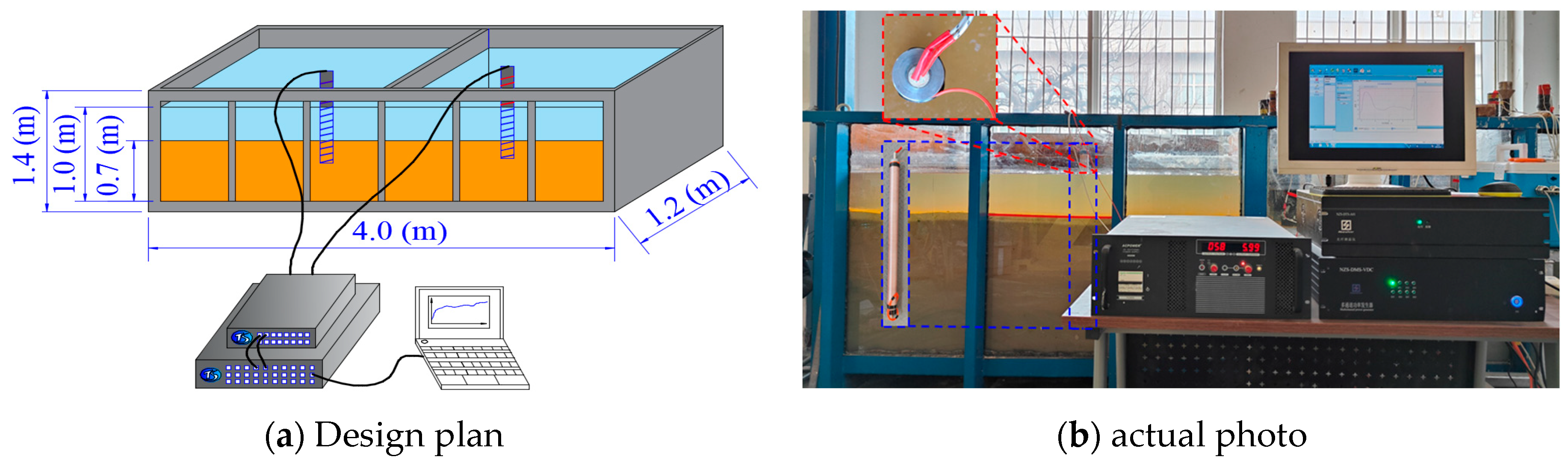
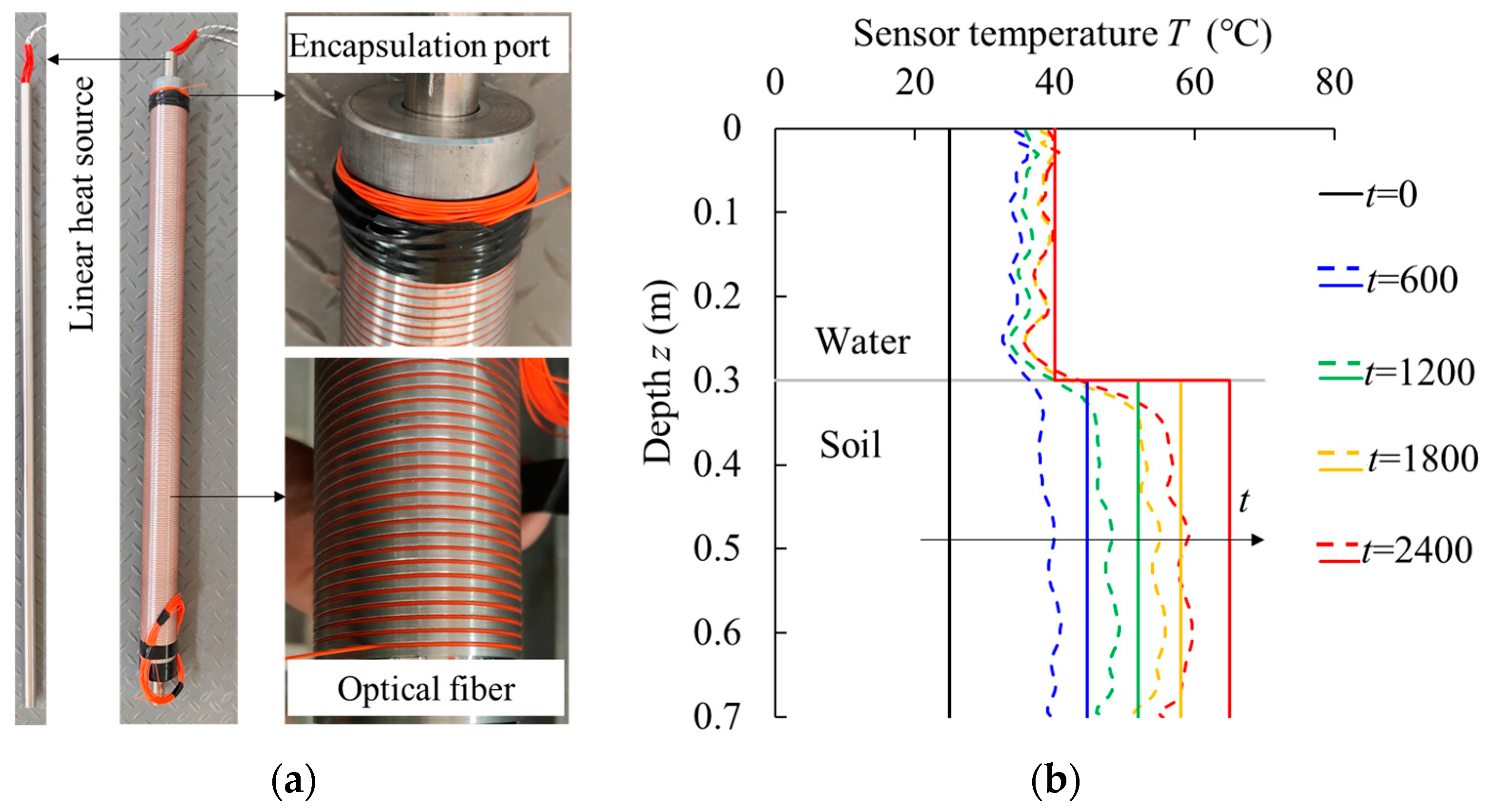
5. Indoor Experimental Verification

To verify the effectiveness of water–soil interface identification based on the non-steady-state heat transfer laws of linear heat sources in water–soil coupled media, this paper relies on the national engineering research center for port water engineering technology of the tianjin water transport science research institute under the ministry of transport, and the key laboratory of port and waterway engineering structure detection, diagnosis and reinforcement technology in the transportation industry. Indoor verification experiments were conducted in the experimental soil tank of the port engineering structure at the port engineering structure test site. The water–soil identification system used in this experiment is shown in Figure 12.

As shown in Figure 12, the water–soil identification system consists of a custom-made experimental tank (dual tank) with a single tank size of 2 m × 1.2 m × 1.369 m, a dynamic temperature data logger (NZS-DTS-A01, Nanzee Sensing, Suzhou, China), a computer, and a heating and temperature sensor. The experiment used kaolin clay, which was mixed with water and stirred into a slurry using a mixer, with a water–soil ratio of 1:1. Before the test, the surrounding environmental temperature was kept constant by using air conditioning. Then, the heating and temperature sensor was pushed into the kaolin clay under the condition that its own temperature was consistent with the ambient temperature. The temperature of the sensor was monitored continuously during the whole test. In the indoor experimental verification, the sensor dimensions were scaled at a 1:2 ratio compared to the prototype dimensions. The model sensor featured a diameter of 5 cm and a length of 70 cm, with a fiber optic pitch of 0.3 cm. The heating power of the linear heat source was configured at 500 W. The details of the sensor are shown in Figure 13. The error percentages between the theoretical and experimental temperatures are shown in

Table 5. The error percentages between the theoretical and experimental temperatures.

Time (s)	Water			Soil
	Theoretical Analysis	Experimental Results	Error (%)	Theoretical Analysis	Experimental Results	Error (%)
t = 600	40.0	34.5	13.8	44.6	36.3	18.7
t = 1200	40.0	36.0	9.9	52.4	44.0	16.0
t = 1800	40.0	38.3	4.3	58.1	49.8	14.3
t = 2400	40.0	38.6	3.6	65.2	53.9	17.3

.

As shown in Figure 13a, the heating and temperature sensor consists of a linear heat source, encapsulation port and optic fiber twining along the trench on the surface of the encapsulation port. Regarding the linear heat source, it is used to lift the temperature of the whole sensor, and the encapsulation port is acting as a connector to combine the linear hear source and the optic fiber. Regarding the optic fiber, it is used to monitor the temperatures of the different positions on the encapsulation port. The differences between the theoretical values (real lines) and experimental values (dashed lines) are displayed in Figure 13b, and the results show that the theoretical values can capture the temperature changing trend and the interface between soil and water. As shown in Table 5, it cannot be denied that there is a certain degree of error between the theoretical calculation results and the experimental results (less than 14% in water and 19% in soil). This is because some details were simplified during the theoretical research process, such as neglecting the radial temperature variation in linear heat sources in the heat transfer process and assuming that linear heat sources are located in a semi-infinite medium. And also, the soil is a porous and discrete medium. In this experiment, the pores within the soil are filled with water, leading to certain changes in the temperature characteristics of the soil during the test. Further research needs to be conducted to update the theoretical calculation in real conditions. There may be certain challenges associated with the application of this method in a marine environment. Nevertheless, since the primary objective is to identify temperature differences between water and soil media, it is noteworthy that the slower temperature increase in seawater and the faster temperature rise in soil will inherently create a more pronounced temperature contrast between the two media. This characteristic could potentially enhance the effectiveness of this method when applied in such settings.

6. Conclusions and Discussion

This study focuses on the dynamic evolution of the erosion of the seabed surrounding offshore structures, considering the differences in thermodynamic parameters of seawater and the seabed soil, and conducts theoretical research on the temperature rise in linear heat sources in water and soil media under a constant heating power. Based on this, theoretical research on the non-steady heat transfer principles in water–soil coupled media is carried out, exploring the theoretical basis and experimental verification methods for water–soil interface identification technology. The research results are of significant importance for improving the accuracy and reliability of sediment monitoring equipment, providing technical support for the operation and management of water transport engineering and offering theoretical support and guidance for the subsequent development of dock slope sediment equipment and the construction of monitoring systems. The main conclusions are as follows:

(1)

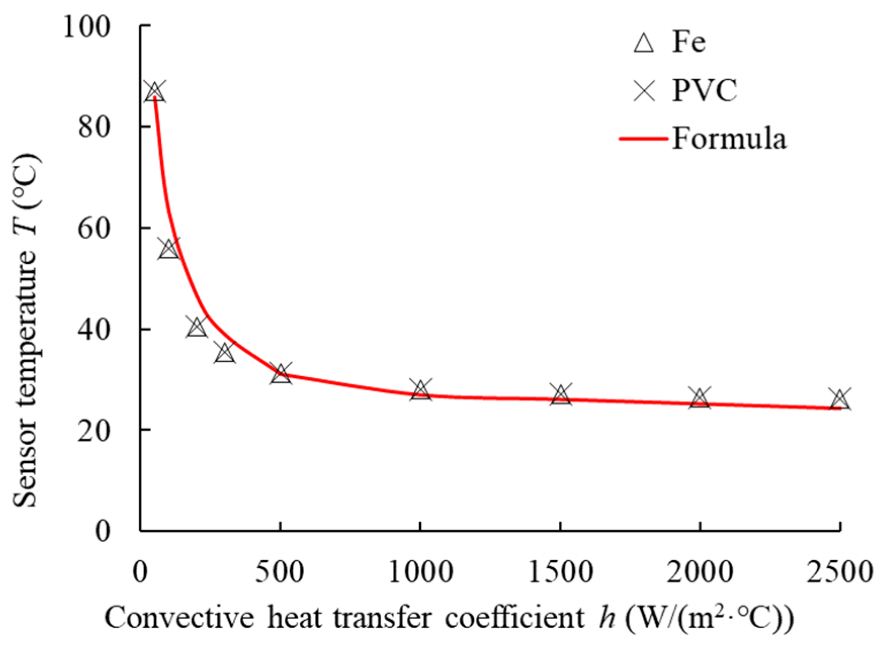
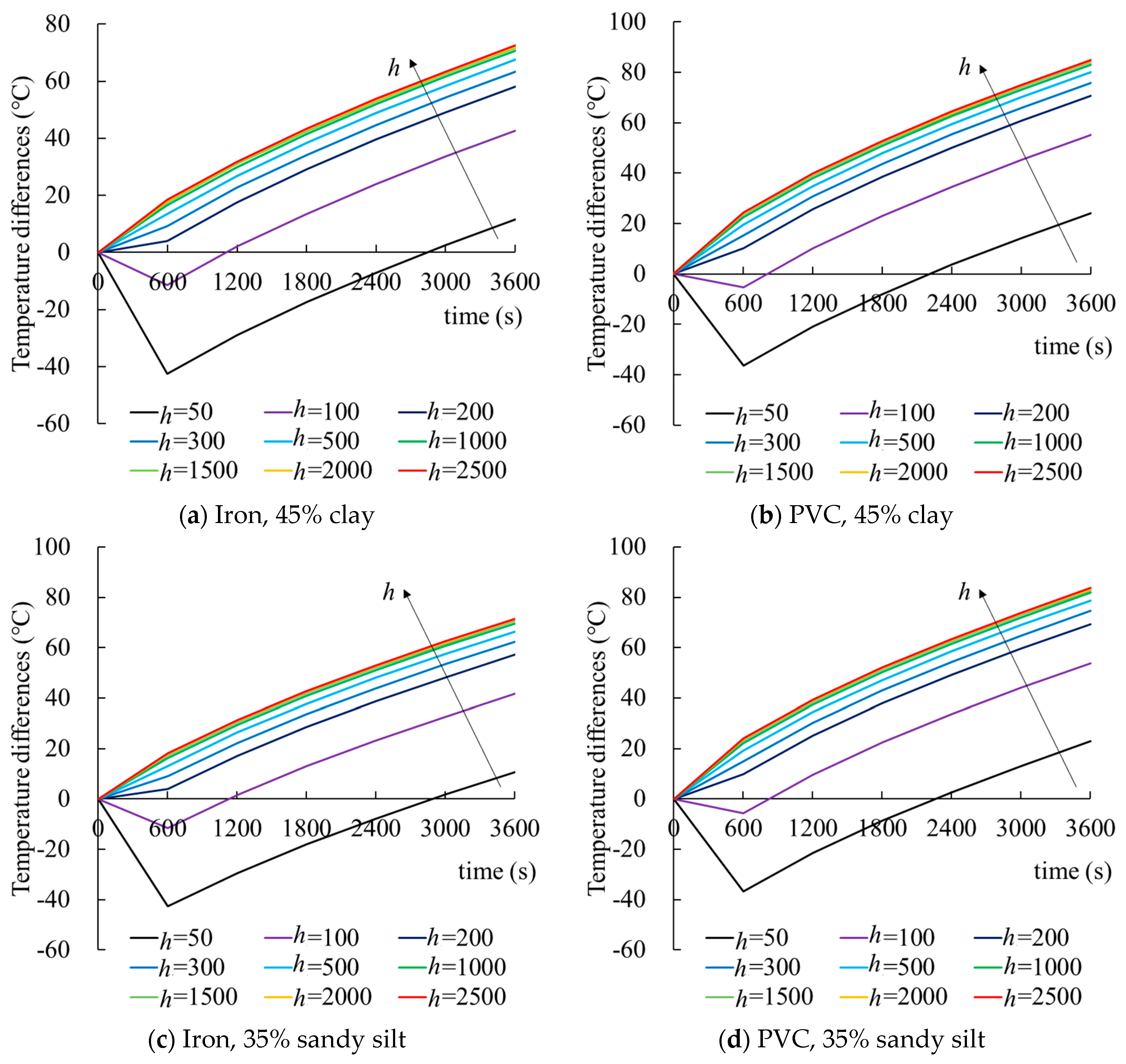
The theoretical formula for the temperature change in a linear heat source in water with constant-power heating is derived. An analysis of iron and PVC heat sources under different seawater convective heat transfer coefficients shows that both materials quickly reach a stable temperature, independent of the material. However, as the convective heat transfer coefficient increases, the heat transferred to seawater rises, causing the stable temperature of the heat source to decrease logarithmically with the convective heat transfer coefficient.

(2)

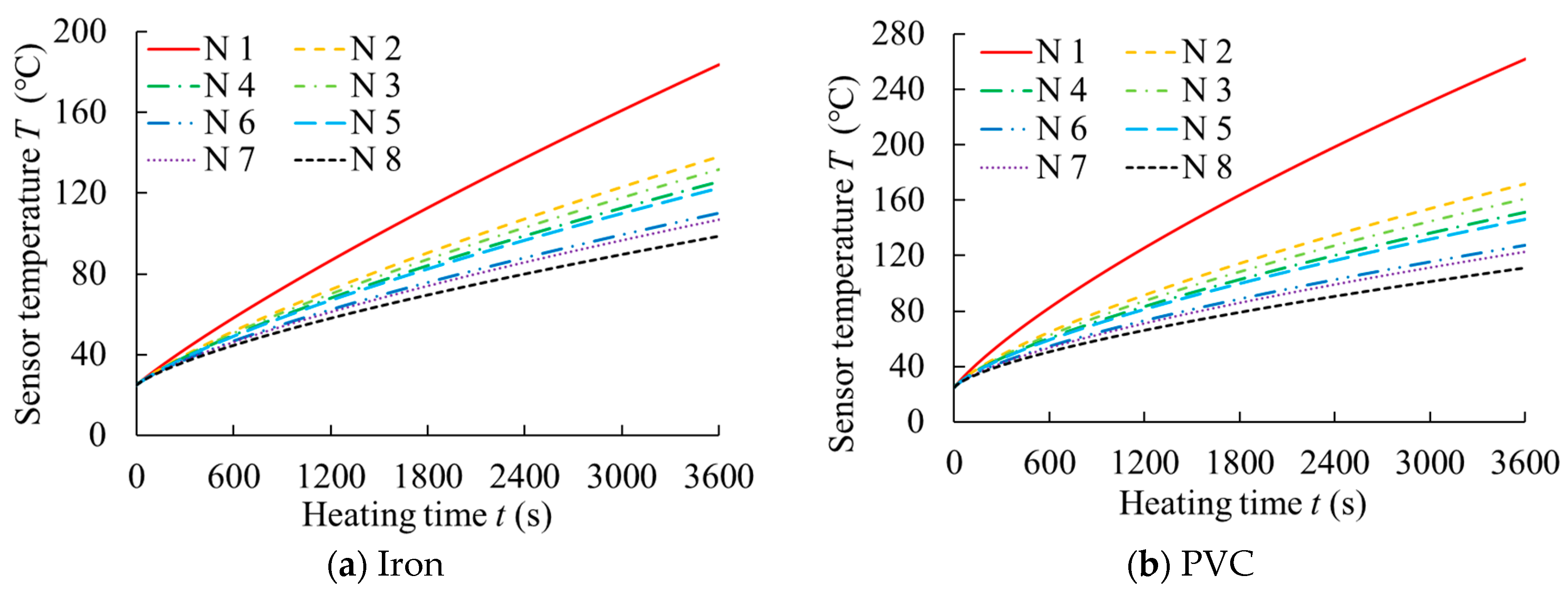
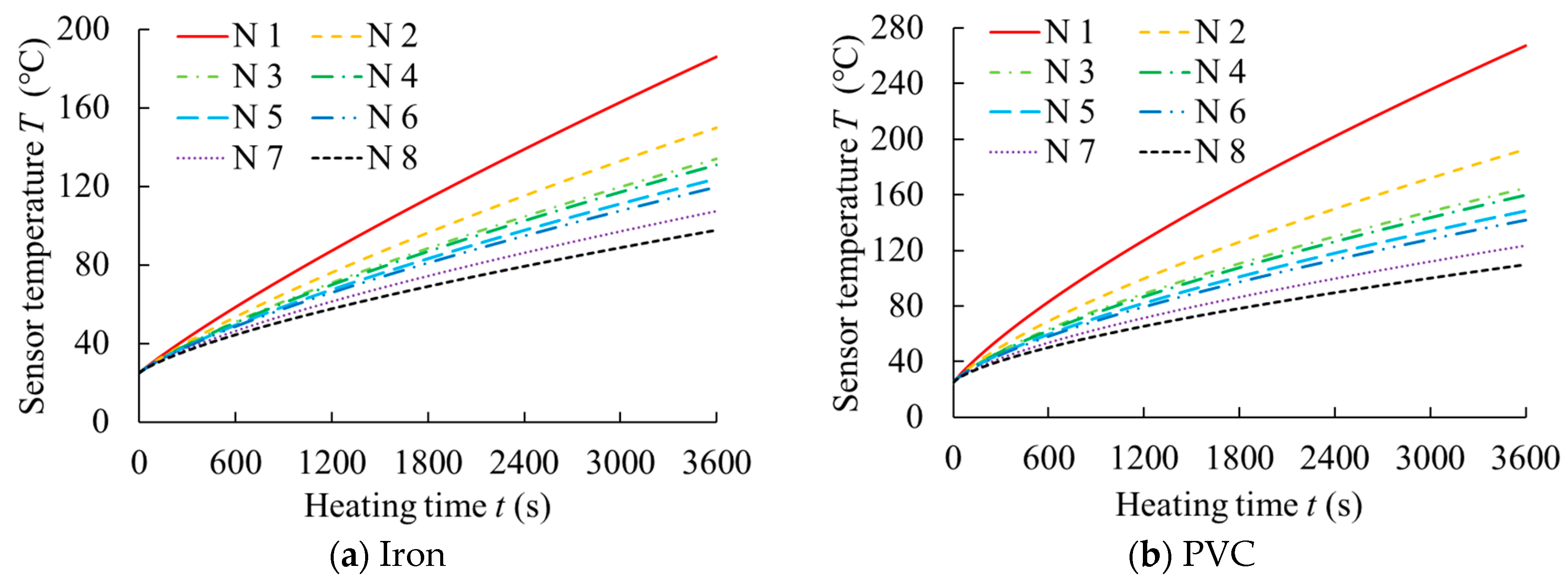
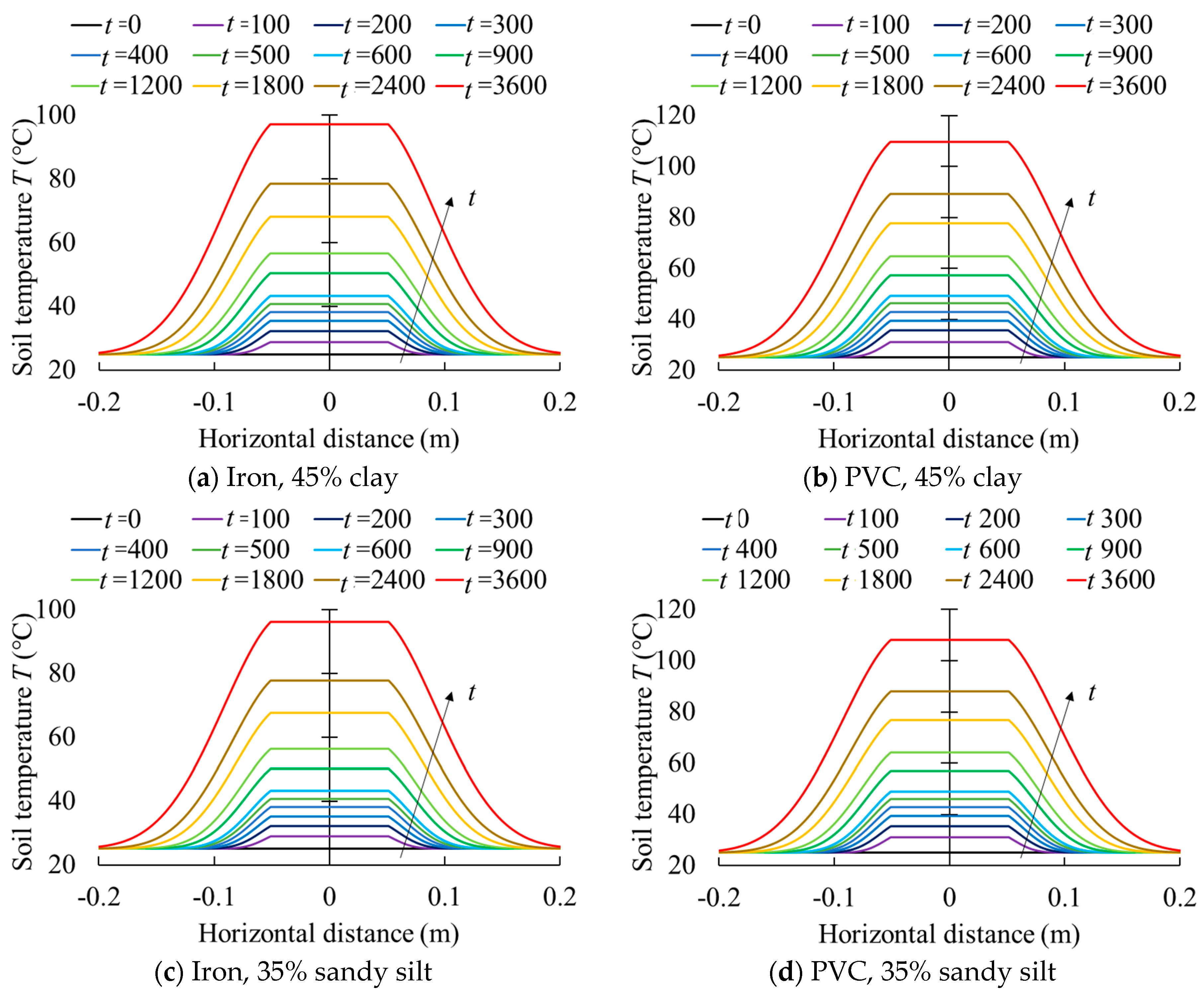
The theoretical formula for the temperature change in a linear heat source in soil under constant-power heating is derived. The temperature response of iron and PVC linear heat sources in eight types of clay and eight types of silt is calculated. The results show that PVC heat sources exhibit a higher temperature change rate than iron in the same soil. Heat transfer from the source to the soil is limited to about 0.2 m after 3600 s. As the heating power increases, temperatures of both PVC and iron sources rise, with a linear relationship between the final temperature and heating power after 3600 s, and the temperature difference between PVC and iron sources gradually widens.

(3)

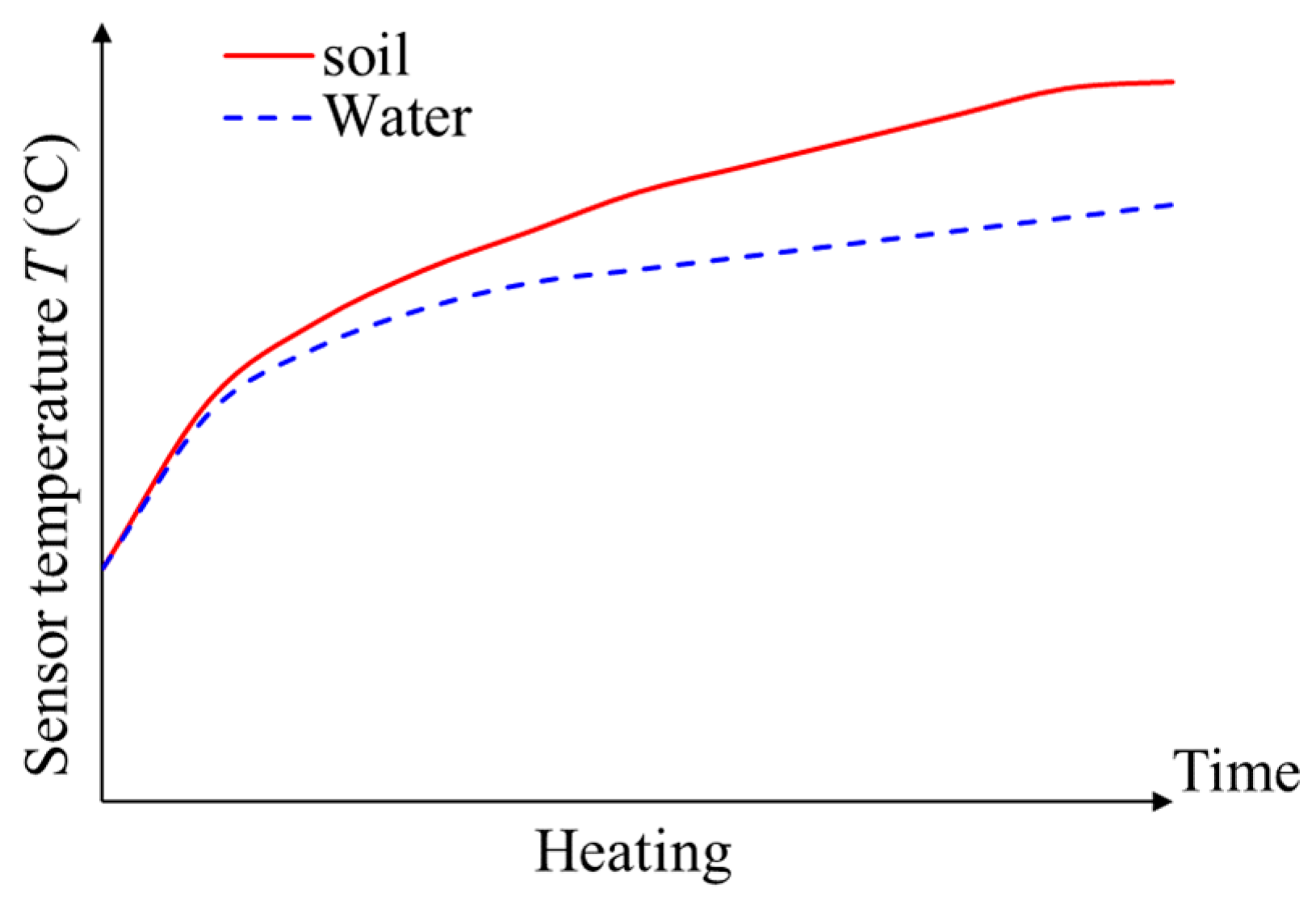
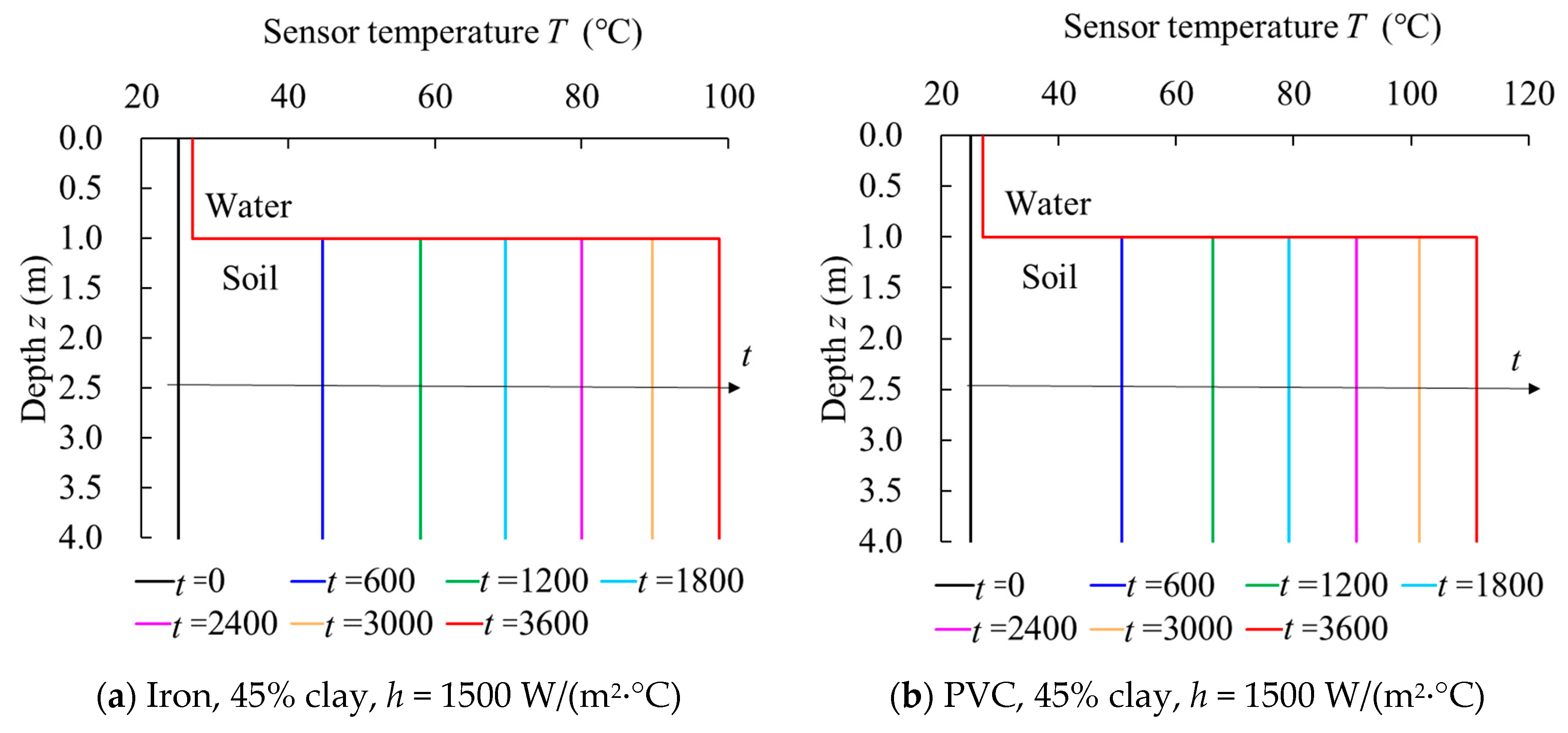
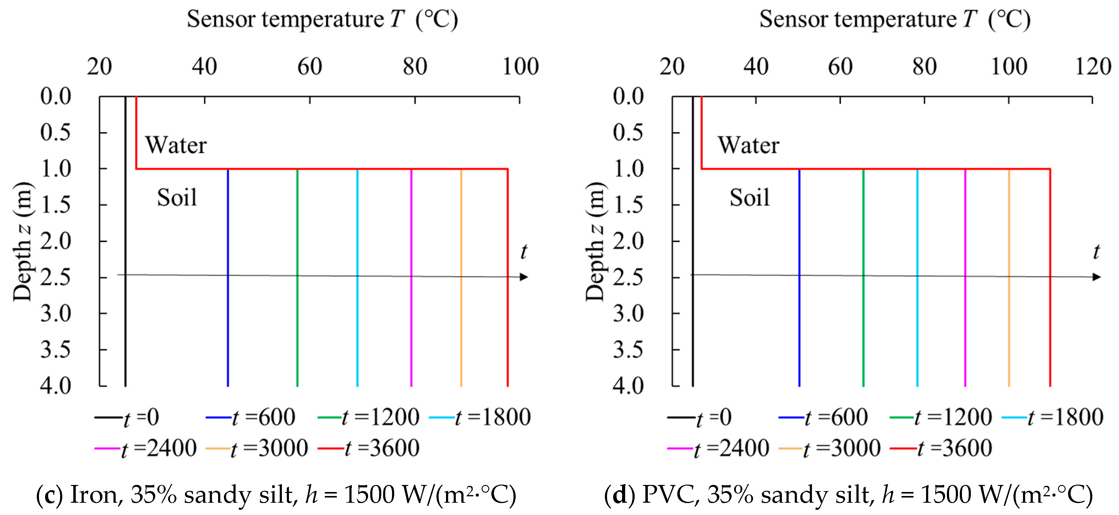
The non-steady heat transfer laws of iron linear heat sources in water–soil coupled media are summarized, highlighting significant temperature differences between water and soil. A clear temperature gradient forms at the water–soil interface, which intensifies with higher convective heat transfer coefficients in water. In soil, slow heat transfer due to low thermal diffusivity results in a gradual surface temperature decrease in the heat source. Conversely, water’s good thermal diffusivity allows for rapid heat transfer, leading to a faster surface temperature decrease. Monitoring surface temperature changes allows for analysis of temperature trends, aiding in distinguishing different medium interfaces and providing a solid theoretical basis for water–soil interface identification.

(4)

The indoor experiments validate the non-steady heat transfer laws for linear heat sources in water–soil media. Monitoring surface temperature changes and analyzing the temperature trends affirm the feasibility of water–soil interface technology based on these laws.

The current study focuses on proposing a framework for monitoring the water–soil interface based on heat transfer theory to identify the dynamic evolution of seabed erosion. Experimental validation has demonstrated that the theoretical framework can be used to identify the water–soil interface. However, due to the idealized assumptions of the theory and the complexity of practical engineering, some details were simplified during the theoretical research process, such as neglecting the radial temperature variation in linear heat sources in the heat transfer process and assuming that linear heat sources are located in a semi-infinite medium, leading to some errors between the experimental validation results and the theoretical results. Future research will delve into the complexity of reproducing actual engineering conditions and explore how to optimize the theoretical model to improve identification accuracy.

References

1. Ni, Y.L.; Gong, M.; Shen, L.D.; Gao, H.X.; Wang, J.B. Coastal evolution and erosion-deposition analysis of underwater slope in Beilun Port. China Harb. Eng. 2017, 37, 27–32. [Google Scholar]
2. Yang, Z.; Li, M.H.; Chen, E.D.; Li, H.; Cheng, S.C.; Zhao, F. Research on the application of BIM-based green construction management in the whole life cycle of hydraulic engineering. Water Supply 2023, 23, 3309–3322. [Google Scholar] [CrossRef]
3. Zhao, C.H.; Zhao, D.J. Application of construction waste in the reinforcement of soft soil foundation in coastal cities. Environ. Technol. Innov. 2021, 21, 101195. [Google Scholar] [CrossRef]
4. Raei, B.; Shahraki, F.; Jamialahmadi, M. Experimental study on the heat transfer and flow properties of γ-Al2O3/water nanofluid in a double-tube heat exchanger. J. Therm. Anal. Calorim. 2017, 127, 2561–2575. [Google Scholar] [CrossRef]
5. Wook, T.K.; Beom, G.P.; Myung, J.L. Thermal performance of glass wool for membrane-type NO96 insulation system in sea water and liquid nitrogen. J. Korean Soc. Mar. Eng. 2017, 41, 807–812. [Google Scholar]
6. Hosseini, M.S.; Mohebbi, A.; Ghader, S. Prediction of thermal conductivity and convective heat Transfer Coefficient of Nanofluids by Local Composition Theory. J. Heat Transf. -Trans. Asme 2011, 133, 052401. [Google Scholar] [CrossRef]
7. Goto, S.; Yamano, M.; Morita, S.; Kanamatsu, T.; Hachikubo, A.; Kataoka, S.; Tanahashi, M. Physical and thermal properties of mud-dominant sediment from the Joetsu Basin in the eastern margin of the Japan Sea. Mar. Geophys. Res. 2017, 38, 393–407. [Google Scholar] [CrossRef]
8. Ahn, K.H.; Jirák, Z.; Knízek, K.; Levinský, P.; Soroka, M.; Beneš, L.; Zich, J.; Navrátil, J.; Hejtmánek, J. Heat capacity and thermal conductivity of CdCr2Se4 ferromagnet: Magnetic field dependence, experiment and calculations. J. Phys. Chem. Solids 2023, 174, 111139. [Google Scholar] [CrossRef]
9. Kandlikar, S.G.; Grande, W.J. Evolution of microchannel flow passages-thermohydraulic performance and fabrication technology. Heat Transf. Eng. 2003, 24, 3–17. [Google Scholar] [CrossRef]
10. Sarafraz, M.M.; Peyghambarzadeh, S.M.; Marahel, A. Mathematical modeling of air duct heater using the finite difference method. Pol. J. Chem. Technol. 2011, 13, 47–52. [Google Scholar] [CrossRef]
11. Su, H.Z.; Tian, S.G.; Kang, Y.Y.; Xie, W.; Chen, J. Monitoring water seepage velocity in dikes using distributed optical fiber temperature sensors. Autom. Constr. 2017, 76, 71–84. [Google Scholar] [CrossRef]
12. Ouellet, V.; Secretan, Y.; St-Hilaire, A.; André et Morin, J. Water temperature modelling in a controlled environment: Comparative study of heat budget equations. Hydrol. Process. 2014, 28, 279–292. [Google Scholar] [CrossRef]
13. Tenchev, R.T.; Falzon, B.G. A pseudo-transient solution strategy for the analysis of delamination by means of interface elements. Finite Elem. Anal. Des. 2006, 42, 698–708. [Google Scholar] [CrossRef]
14. Lin, G.; Li, P.; Liu, J. Transient heat conduction analysis using the NURBS-enhanced scaled boundary finite element method and modified precise integration method. Acta Mech. Solida Sin. 2017, 30, 445–464. [Google Scholar] [CrossRef]
15. Doughty, C.; Pruess, K. A similarity solution for two-phase water, air, and heat flow near a linear heat source in a porous medium. J. Geophys. Res. Solid Earth 1991, 97, 1821–1838. [Google Scholar] [CrossRef]
16. Incropera, F.P.; De Witt, D.P. Fundamentals of Heat and Mass Transfer, 2nd ed.; Staff. Gen. Res. Pap.; John Wiley & Sons, Inc.: Hoboken, NJ, USA, 1981; Volume 27, pp. 139–162. [Google Scholar]
17. Zhang, W.C.; Zhang, Y.L. Active heat method with distribution fiber temperature sensing for suspension location of submarine power cable. J. Harbin Univ. Sci. Technol. 2020, 25, 47–52. [Google Scholar]
18. Guerrero, J.S.P.; Pontedeiro, E.M.; van Genuchten, M.T.; Skaggs, T.H. Analytical solutions of the one-dimensional advection–dispersion solute transport equation subject to time-dependent boundary conditions. Chem. Eng. J. 2013, 221, 487–491. [Google Scholar] [CrossRef]
19. Zhao, X.F.; Li, W.J.; Zhou, L.; Song, G.; Zhu, Z.; Du, J. Application of support vector machine for pattern classification of active thermometry-based pipeline scour monitoring. Chin. J. Nurs. 2015, 22, 903–918. [Google Scholar] [CrossRef]
20. Zhao, X.F.; Li, L.; Ba, Q.; Ou, J.-P. Scour monitoring system of subsea pipeline using distributed Brillouin optical sensors based on active thermometry. Opt. Laser Technol. 2012, 44, 2125–2129. [Google Scholar] [CrossRef]
21. Day, W.A. Time versus distance for the propagation of heat in bounded domains. Q. Appl. Math. 2000, 58, 325–330. [Google Scholar] [CrossRef]
22. Deo, B.B.; Behera, S.N. Calculation of thermal conductivity by the kubo formula. Phys. Rev. 1965, 141, 738–741. [Google Scholar] [CrossRef]
23. Michele, S.; Borthwick, A.G.L. The laminar seabed thermal boundary layer forced by propagating and standing free-surface waves. J. Fluid Mech. 2023, 956, A11. [Google Scholar] [CrossRef]
24. Michele, S.; Stuhlmeier, R.; Borthwick, A.G.L. Heat transfer in the seabed boundary layer. J. Fluid Mech. 2021, 928, R4. [Google Scholar] [CrossRef]
25. Postolnik, Y.S.; Manko, V.M. Calculation formula for experimental determination of temperature-dependent coefficient of thermal conductivity. Recon Tech. Rep. N 1983, 83, 109–112. [Google Scholar]
26. Berdnikov, V.S.; Grishkov, V.A.; Markov, V.A. The propagation of temperature pulsations along the free surface of a liquid layer from a linear heat source. J. Phys. Conf. Ser. 2019, 1382, 012077. [Google Scholar] [CrossRef]
27. Lo, Y.L.; Xu, S.H. New sensing mechanisms using an optical time domain reflectometry with fiber Bragg gratings. Sens. Actuators A-Phys. 2007, 136, 238–243. [Google Scholar] [CrossRef]
28. Cangialosi, C.; Girard, S.; Cannas, M.; Boukenter, A.; Marin, E.; Delepine-Lesoille, S.; Marcandella, C.; Paillet, P.; Ourdane, Y. Raman based distributed fiber optic temperature sensors for structural health monitoring in radiation environment. In Proceedings of the 2015 15th European Conference on Radiation and Its Effects on Components and Systems (RADECS), Moscow, Russia, 14–18 September 2015. [Google Scholar]
29. Jiang, M.S.; Sui, Q.M.; Lin, Z.Q. Application of distributed fiber optic temperature sensor system in oil field logging. Opt. Fiber Electr. Cable Their Appl. 2007, 2, 29–31. [Google Scholar]
30. Shahsafi, A.; Roney, P.; Zhou, Y. Temperature-independent thermal radiation. Proc. Natl. Acad. Sci. USA 2020, 116, 26402–26406. [Google Scholar] [CrossRef] [PubMed]
31. Chen, Q.; Huang, Y. Effect of low wick permeability on transient and steady-state performance of heat pipes. Heat Transf. Res. 2019, 50, 1319–1332. [Google Scholar] [CrossRef]
32. Sivaprasad, A.; Basu, P. Comparative assessment of transient- and steady-state soil thermal conductivity using a specially designed consolidometer. Geothermics 2022, 107, 102583. [Google Scholar] [CrossRef]
33. Kolenda, Z.S.; Szmyd, J.S.; Huber, J. Entropy generation minimization in steady-state and transient diffusional heat conduction processes Part I—Steady-state boundary value problem. Bull. Pol. Acad. Sci.-Tech. Sci. 2015, 62, 875–882. [Google Scholar] [CrossRef]
34. Trcala, M.; Cermák, J.; Nadezhdina, N. Water content measurement in tree wood using a continuous linear heating technique. Int. J. Therm. Sci. 2015, 88, 164–169. [Google Scholar] [CrossRef]
35. Trcala, M.; Cermák, J. A new heat balance equation for sap flow calculation during continuous linear heating in tree sapwood. Appl. Therm. Eng. 2016, 102, 532–538. [Google Scholar] [CrossRef]
36. Van Bockstal, K.; Slodicka, M. Recovery of a time-dependent heat source in one-dimensional thermoelasticity of type-III. Inverse Probl. Sci. Eng. 2017, 25, 749–770. [Google Scholar] [CrossRef]
37. Abdoh, D.A. Peridynamic modeling of transient heat conduction in solids using a highly efficient algorithm. Numer. Heat Transf. Part B-Fundam. 2024, 2024, 2310708. [Google Scholar] [CrossRef]
38. Bobaru, F.; Duangpanya, M. The peridynamic formulation for transient heat conduction. Int. J. Heat Mess Transf. 2010, 53, 4047–4059. [Google Scholar] [CrossRef]
39. Xi, Q.; Zhong, J.X.; He, J.X. A Ubiquitous thermal conductivity formula for liquids, polymer glass, and amorphous solids. Chin. Phys. Lett. 2020, 37, 104401. [Google Scholar] [CrossRef]
40. Jennings, S.; Hasterok, D.; Payne, J. A new compositionally based thermal conductivity model for plutonic rocks. Geophys. J. Int. 2019, 219, 1377–1394. [Google Scholar] [CrossRef]
41. Bessrour, J.; Bouhafs, M.; Khadrani, R. Heat transient model for surface treatment by a moving laser source. Int. J. Therm. Sci. 2022, 41, 1055–1066. [Google Scholar] [CrossRef]
42. Chang, S.P.; Zhang, S.M. Engineering Geology Handbook; China Architecture & Building Press: Beijing, China, 2007. [Google Scholar]
Figure 1. A schematic diagram of heating and cooling in water and soil media.
Applsci 14 04686 g001
Figure 2. Schematic diagram of monitoring equipment.
Applsci 14 04686 g002
Figure 3. Temperature rise curve of linear heat sources in seawater.
Applsci 14 04686 g003
Figure 4. The relationship between the final steady-state temperature of a linear heat source in seawater and the convective heat transfer coefficient h.
Applsci 14 04686 g004
Figure 5. Temperature change law during heating process of clayey soil.
Applsci 14 04686 g005
Figure 6. Final temperature of clayey soil at 3600 s of heating.
Applsci 14 04686 g006
Figure 7. Temperature change law during heating process of silty soil.
Applsci 14 04686 g007
Figure 8. Final temperature of silty soil at 3600 s of heating.
Applsci 14 04686 g008
Figure 9. The distribution of the soil temperature field during the heating process.
Applsci 14 04686 g009
Figure 10. The temperature distribution of the heat source in a water–soil coupled medium under different convective heat transfer coefficients.
Applsci 14 04686 g010aApplsci 14 04686 g010b
Figure 11. Temperature difference in water–soil coupled media with linear heat sources of different convective heat transfer coefficients.
Applsci 14 04686 g011
Figure 12. The water–soil identification system.
Applsci 14 04686 g012
Figure 13. The details of the heating and temperature sensor and the relevant temperature changes. (a) The details of the heating and temperature sensor. (b) The temperature changes in the testing and analytical solution.
Applsci 14 04686 g013