Abstract
The mechanical description of the failure of quasi-brittle materials is a challenging task. Rocks, concrete, ceramics, and natural or artificial composites could be considered for this material classification. Several characteristic phenomena appear as emergent global behaviors based on the interaction of many simple elements, such as the effect of size and the interactions between micro-cracks. These are essential features of a complex system. These topics were investigated using acoustic emission techniques and a numerical approach that used a continuum media hypothesis called peridynamics. In this context, a pre-notched concrete specimen was manufactured. A mechanical test was performed to acquire acoustic emission signals. The problem was also simulated using the peridynamic model. The evolution of the damage process, which is presented in terms that go beyond only the global reaction vs. displacement and the evolution of the acoustical emission global parameter, is presented. Finally, the synergy between the experiments and simulations is discussed.
1. Introduction
The interactions among a cluster of micro-cracks, the localization effect, and the effect of size characterize the damage process in a quasi-brittle material. Concrete, rocks, ceramics, and artificial composite materials are examples of this kind of material. An important characteristic of these materials is that the damage governs the way in which system failure occurs. Many researchers have studied the damage process, finding interesting results within the theory of continuum mechanics aided by the branch of plasticity. Studies that have used this approach can be found in the classic book by [1] and in the reviews presented by [2,3], which also utilized the same methodology as in [4], where a failure law for a metal alloy based on continuum damage mechanics is presented. In [5], a different point of view is presented, whereby the random nature of material properties and the use of discrete methods are considered as alternative strategies. Several discrete element-based approaches are available in the technical literature. Among others, two literature review papers can be cited: [6] in 2015 and [7] in 2019. In the present work, the discrete method used is a computational implementation of a peridynamic theory proposed by [8]. In [9], a damage law in the context of the peridynamics is presented. This method is now used in several applications, as has been presented in [10], among other references. In the present work, this technique is applied to simulate pre-notched concrete specimens and study their mechanical behavior until collapse. The novelty of the peridynamic model is in simulating the acquisition of acoustic emission data during the test. In the discussion of the results, several observations are made to illustrate the possibilities of using simulation with this approach to complement the understanding of the damage process in real structures.
In agreement with this approach to solving the problem, considering mechanical collapse governed by fracture as a phase transition problem could be interesting. Phase transition is typically used in the statistical physics branch of modern physics, as presented in many classical books, such as [11]. Several prestigious researchers in solid mechanics share this point of view, such as [12,13,14,15,16].
The normalization group method proposed by [17] explains this universal behavior. The practical implication of this characteristic behavior in the context of the failure of materials implies that when a system is close to local or global collapse during its damage process, the global parameters that govern the system follow potential laws with characteristic exponents. Then, when these global parameters adopt a potential shape with a characteristic value, global or local collapse is imminent.
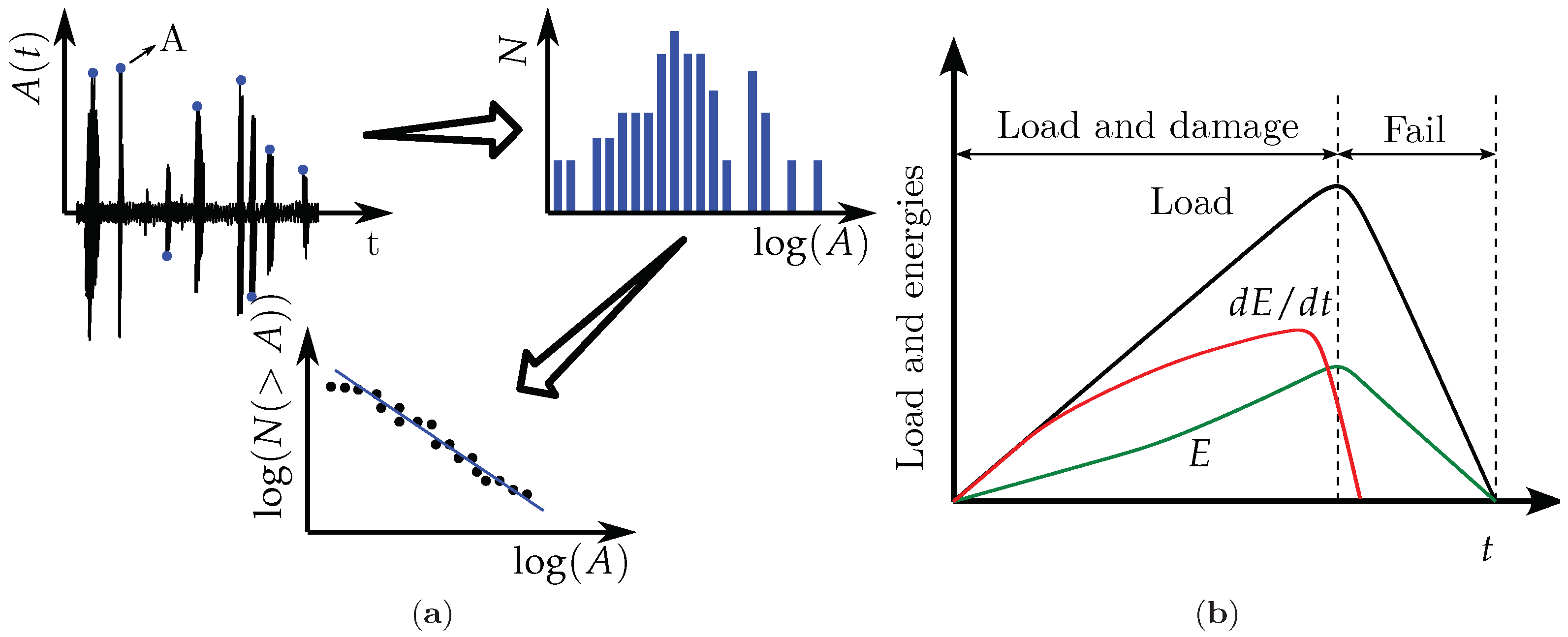
In [13], the statistical distribution of seismic magnitude from 1985 to 1998 in Japan was plotted as a log–log axis, and a potential law between the number of events and their magnitude naturally appeared. If all of the interval is included in the plot, a potential expression with an exponent of 0.88 appears clearly, as depicted in Figure 1. The exponent of 0.6 emerges when the time interval is reduced close to a significant seismic event. In the present case, the interval used to compute the interval close to the collapse was 0–100 days; then, in this time window, the statistical distribution of seismic magnitudes is defined by a potential law with this characteristic exponent (0.6). Figure 1 illustrates this phenomenon (originally presented in [13]), which has been adapted in the present work.
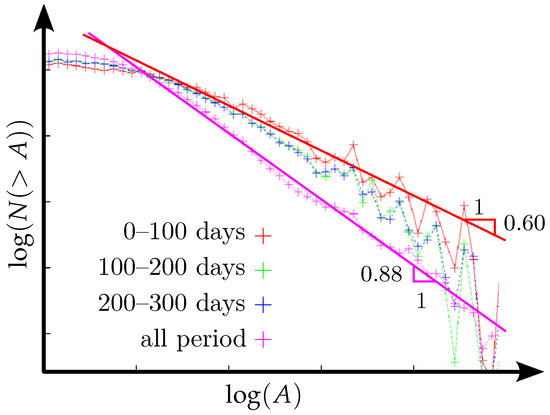
Figure 1.
The relation between the statistical distribution (N (>A)) of events during seismic evolution in Japan and the amplitude (A) for the period 1985–1998 is examined. This demonstrates how closely the main shock occurs on day 0, as well as the change in the exponent from 0.88 for the entire period to 0.6 for a period close to the main shock.
This situation has also been clarified by [15] when using the bundle method, where the geometric and boundary conditions of the problem studied are significantly simplified, using a set of elastic parallel bounds with random strength fixed in two rigid supports.
The bundle model provides insight into how to lead fractures in solids using the phase transition point of view, showing that, in this case, the order parameter could be linked to the statistical distribution of the avalanches (parts of the structure that present a local collapse inside the structure). Gutenberg and Ritcher proposed this kind of law in the 1950s [18] in the context of seismology.
In [19], the analysis of this kind of problem as a “crackling noise problem” was considered, viewing it as a typical set of problems that could be analyzed in the framework of renormalization group theory.
This law was also successfully used to relate the magnitude of signals to their frequency in an acoustic emission (AE) test. AE is a technique used today to measure the characteristics of the structure used. Essentially, the mechanical waves produced by an internal change in the structure (called AE events, produced by damage, corrosion, or another source) are captured as signals by surface devices. The analysis of the signal captured with the AE devices lets researchers know the spatiotemporal distribution of the events in the process studied.
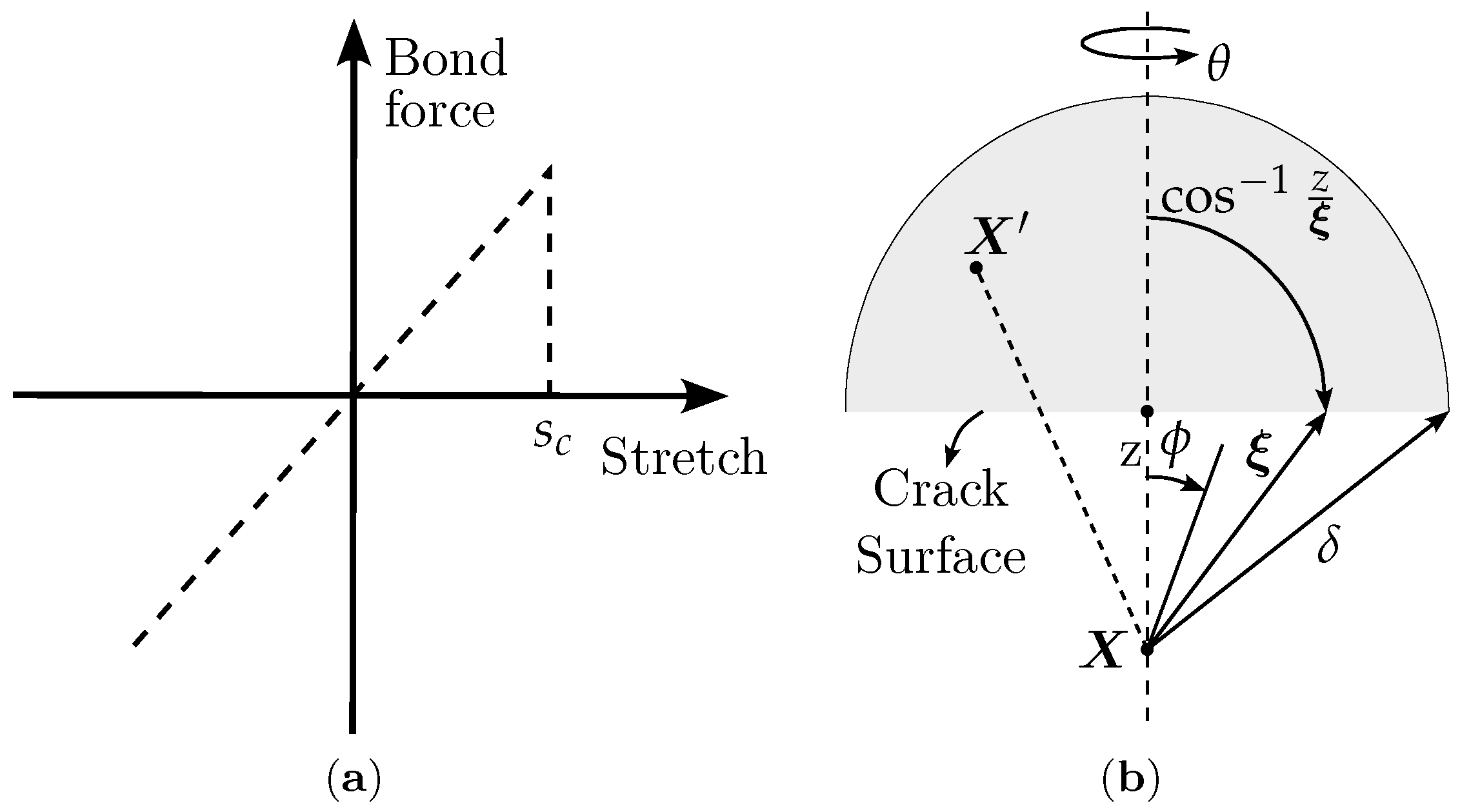
A basic reference for the AE technique used in structures built with quasi-brittle materials is [20]. The distribution of signals during damage evolution is classical information that can be used directly to characterize the damage process. A measure of the energy distribution produced by the events, which is computed as the area below each signal, is also considered rich information with which to describe the damage process. The so-called b-value is a classical parameter that emerges to generalize the Gutenberg–Ritcher law.
The link between the amplitude of the signals and their statistical accumulated distribution can be written as follows:
where A indicates the amplitude of the AE signals, N is the accumulated number of signals, and b represents the coefficients. The meaning of the b-value is explained in Figure 2a. Several scientific publications determined that the b-value, which is the exponent of a potential law, has a sensible fall in its value when the eminence of local or global collapse is near. See the classical book [12] as a reference.

Figure 2.
(a) An example of device record vs. time. AE signal statistical density and the accumulated number of signals plotted on an axis in a log–log scale, where the b-value coefficient presented in Equation (1) can be seen. (b) The DPH index is represented in schematic form by the red curve.
A proposal to link the b-value to the fissure fractal dimension, D, was presented by [21] and previously in [22]. A simple expression, , is proposed. Then, when b is around 1.5, the signal is emitted from the entire dominion, ; when the b-value falls, this indicates that D tends to concentrate the AE emission to the localized surface region, , which is linked to the abrupt release of a high quantity of energy, a phenomenon associated with local or global collapse. An application of the b-value and fractal dimensions can be seen in [23], whereby the failure of concrete under compression was investigated using two semi-empirical Gutenberg–Richter (GR) laws.
Other precursors have been computed from AE signals; among many of the important options is the natural time approach proposed by [24]. In these books, the authors presented several indices computed from data signals that could be applied in the AE context.
Dȩbsky, Pradhan, and Hansen [25] presented an interesting computed precursor regarding the evolution of the elastic energy temporal derivative during system evolution, which they called the DPH index. The authors proposed that a local or global maximum value in the DPH index is a precursor, and increasing its value is associated with the eminence of local or global damage in the system studied. This can be seen in schematic form in Figure 2b, where the link between this index and system collapse is presented. In the original work of [25], this index was computed with numerical results, making the study of elastic energy evolution available. In [26], this idea was generalized by considering the fact that the product of the support-prescribed displacement and the corresponding reaction is proportional to the elastic energy stored in the system during the test. The performance of the cited index applied to a real problem is shown. The DPH index provides complementary information when an AE test is applied.
The goal of the present study is to analyze the damage process in a body using (i) AE information, (ii) DPH index evolution, and (iii) peridynamic simulation as complementary information to interpret the AE data. We believe that the primary contribution of this work will be to demonstrate the effectiveness of the DPH index and numerical simulation of acoustic emission using a peridynamic model. This could be a crucial alternative to help interpret the AE information collected in these kind of tests.
After the present introduction, the fundamental characteristics of the peridynamic method are shown in Section 2. Then, in Section 3, the application of the model is described, and the details of the experimental test are depicted. Section 4 explains the details of the numerical simulation using the peridynamic model. In Section 5, the experimental and numerical results are presented, and we present a discussion that attempts to illustrate how using peridynamic simulation and the DPH index could complement the information obtained from AE data. Finally, the conclusions about the analysis performed are presented.
2. Bond-Based Peridynamic
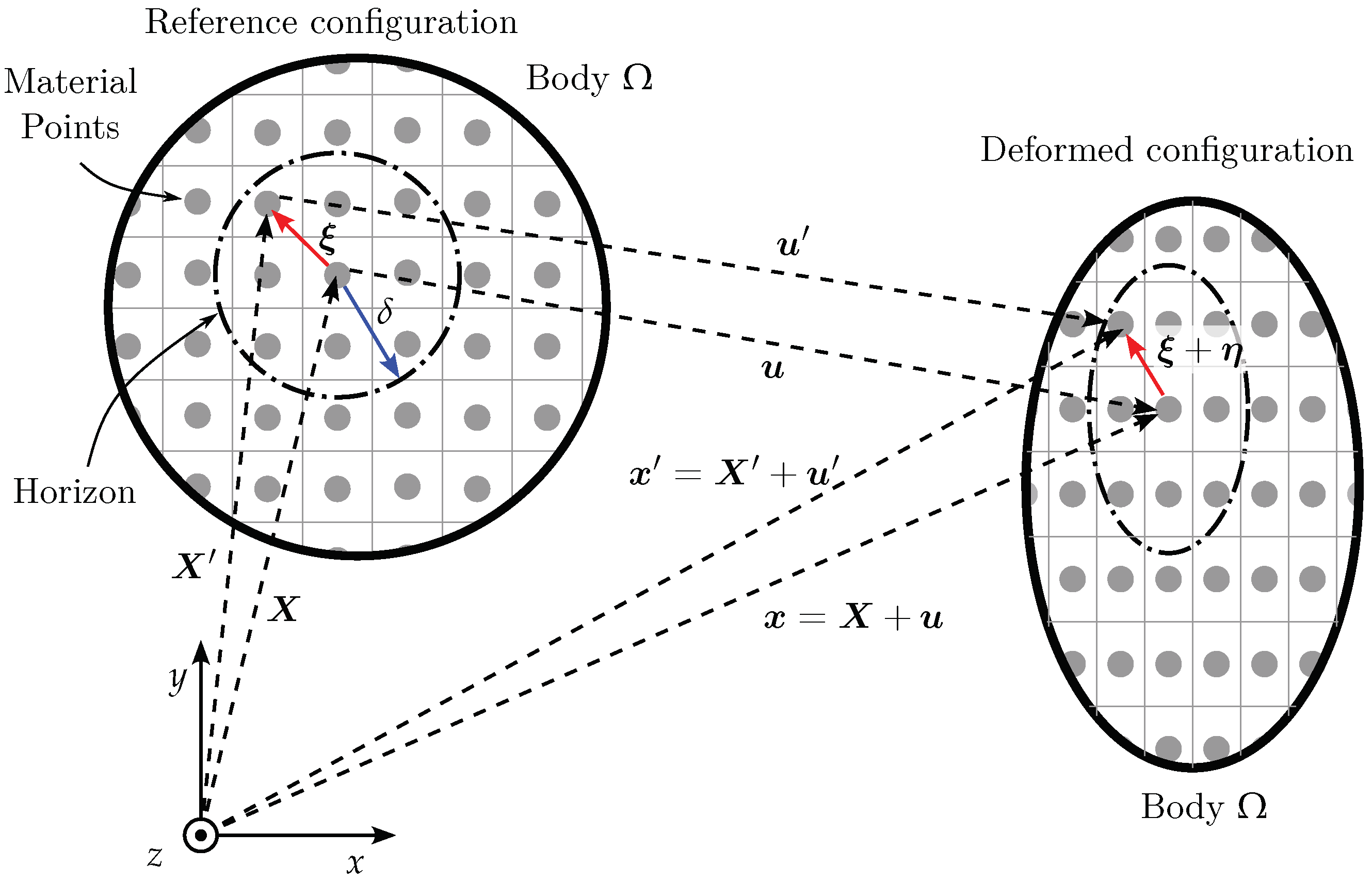
Peridynamic theory is a non-local formulation of the continuum media that uses spatial integration to describe the internal discretization of the material points. This characteristic became adequate for simulating the emergence of discontinuities produced by spontaneous initiation and fissure propagation. The bond-based formulation proposed by [8] is presented as the first kinematic field variable; the displacement or the strain field used in continuum mechanics released the necessary restriction to accomplish the continuum media hypothesis.
In the bond-based formulation, each material point, , can interact with other material points, , inside a determined distance, , called the horizon, as presented in Figure 3. Considering the interaction between the two points and in the non-deformed configuration, the relative position is given for . Where strain occurs in the region, the points and will suffer displacement, , and having its new position determined for and , where the relative displacement is and the relative position is .
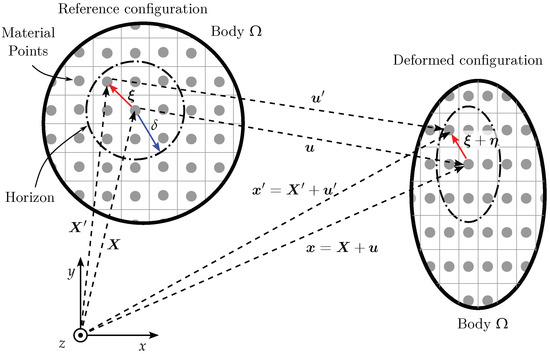
Figure 3.
The interaction between two material points in the bond-based model. The arrow with blue color represents the horizon () and arrows with red color represents the distance between material points and .
The motion equation within peridynamic theory up to Newton’s second law is written as follows:
where is a force function exerted for the link between a pair of points, and , and represents the body force in point . The force function exerted for the bound must contain the material’s constitutive information; then, we use the proposal presented in [8] for a micro-elastic material. must be derived for a scalar function, ; then,
where must represent the elastic strain energy for the volume stored in the material, and this can be defined as
In Equation (4), the function represents the bound micro-module; it is a parameter related to the material, which can be considered as constant. represents the bound displacement and can be expressed in the following manner:
where represents the distance between the material points linked by a bound in the non-deformed configuration, and represents the distance between the same material points in the deformed configuration. This substitutes Equation (5) in Equation (4), where we obtain the function that defines the force exerted for the link between the pair of material points and in the bond-based formulation for an isotropic linear elastic:
The micro-module of the link for a linear material with three dimensions was defined by [9] as
where E represents Young’s modulus and is Poisson’s ratio.
In the bond-based formulation, the damage is introduced by means of eliminating the interaction between the material points. When the link stretch between a pair of material points ( and ) reaches a critical value, , this link is deactivated. In Figure 4a, this law is depicted. This procedure is reflected in Equation (2) through removing the bound force function that links the points and , resulting in force redistribution among the already active links. In order to associate the critical strain with known material properties, ref. [9] propose that the total work of all the links that cross the crack surface must be equal material fracture toughness, , when these bounds stay with their strain equal to the critical strain, as shown in Figure 4b. This proposal can be expressed as
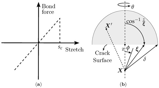
Figure 4.
(a) Damage law. (b) Integration domain of the links that cross the crack surface.
Rearranging Equation (8), it is possible to obtain critical stretch as a function of material toughness for a 3D problem:
In order to include damage in the material response, Equation (6) can be altered, including the scalar function , taking into account the damage level in the bound.
The function can be written as follows:
The damage state associated with a material point, , can be computed using the ratio between the number of links eliminated () and the total number of links that arrive at point :
In order to improve the behavior of real materials, toughness is represented as a random field with a Weibull distribution, given for
where and are parameters that govern the scale and shape of the Weibull distribution. Details about how to carry out the computational implementation of as a random field are explained in [27].
3. Experimental Tests
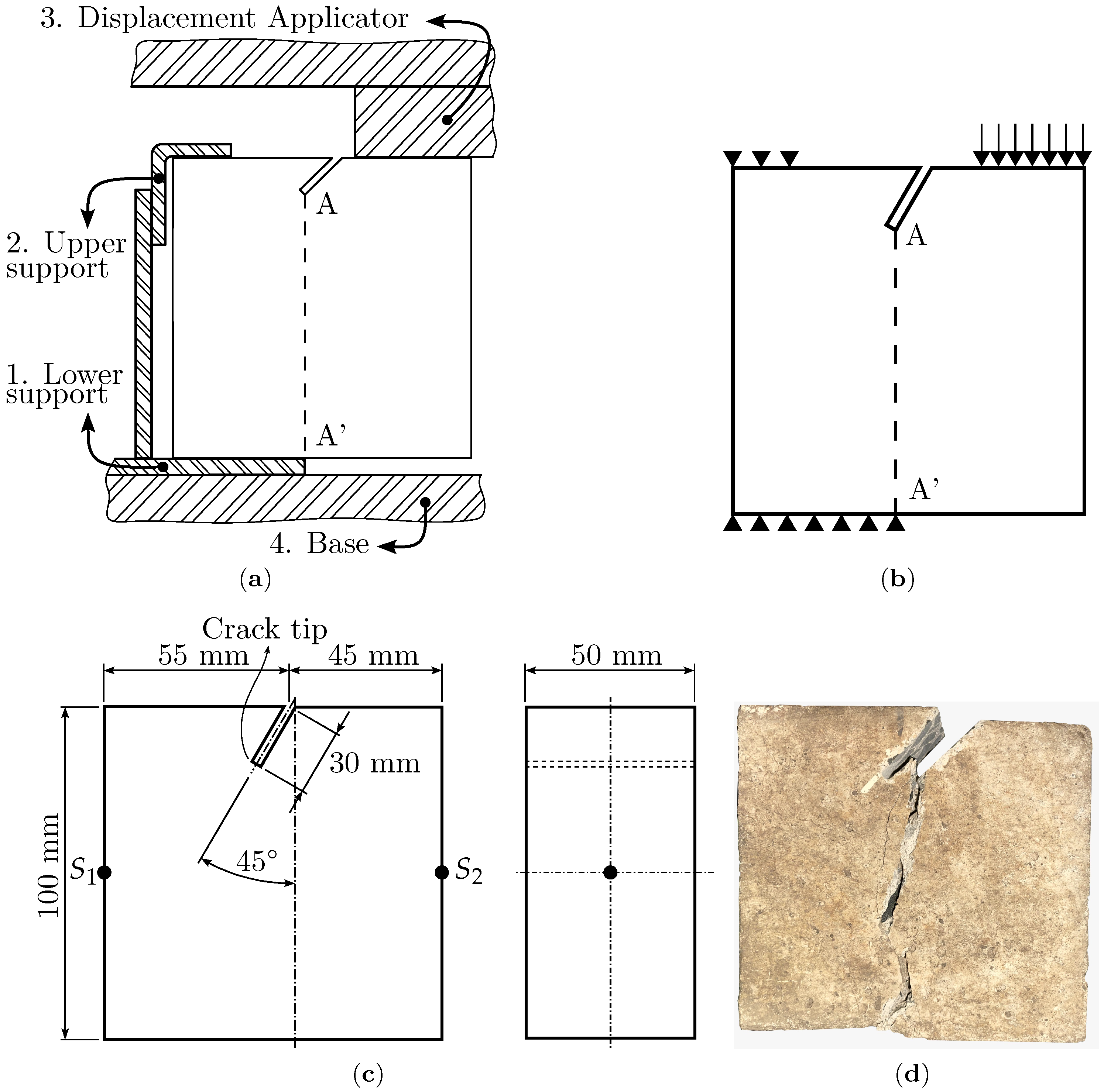
The present work analyses a pressured prismatic concrete body. The supporting details used to test the body are presented in Figure 5a. The boundary conditions used in the test are depicted in Figure 5b. In addition, in Figure 5c, the dimensions, the geometric details of the concrete specimen, and the positions of sensor 1 () and sensor 2 () are presented. One of the specimens after carrying out the test is shown in Figure 5d.
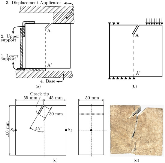
Figure 5.
Information about the test performed: (a) the fixer dispositive used in the test, (b) the boundary conditions used in the test, and (c) the dimensions that characterize the test specimen. (d) Failure specimen.
Notice that, as indicated in Figure 5, points A (the place where the fissure initiates) and A’ (the point where the fixing is in the lower support) are aligned in the vertical direction. The superior rigid block depicted as (3) in Figure 5a applies a prescribed displacement at a constant velocity of mm/ acting in line A to A’, as presented in Figure 5b. The universal test machine used was a Shimadzu AGX-PLUS, which has a proprietary data recording system that is used to record load and displacement at a sample rate of 100 / [28]. Piezoelectric crystals with resonance frequencies of were placed on the specimen at positions and , as indicated in Figure 5c. The sensors were connected to the Omega® OM-USB data-acquisition set, with a sampling ratio of 300 / and a 12-bit resolution. The data were collected continuously. The AE signals were identified throughout the data post-processing process.
Notice that a standard procedure was not used to perform this experimental test; however, as will be shown in Section 5, the flexibility of the left upper support induces great variability among the result tests. This characteristic was useful in illustrating how the interpretation of the AE results could be improved using numerical simulation and the DPH index.
4. Numerical Analyses Using Peridynamic Model
The input data for the peridynamic model consist of the mechanical properties, geometry, and boundary conditions, as depicted in Figure 5b. The mechanical properties that characterize the model are (i) Young modulus (E) and (ii) critical stretch (), as defined in Equation (9), (iii) fracture toughness (), and (iv) material density ().
The computational implementation of the peridynamic model used is based on the Fortran code described in the book of Madenci and Oterkus [29]. In this model, critical stretch, , is computed using Equation (9), and it is defined as a function of the parameters E, , and the horizon, , which is a material characteristic length. The horizon represents the number of nodes that will be connected through bounds, as depicted in Figure 4. The meaning of this material characteristic length is discussed in [30,31] and in the context of the discrete element methods in [32,33]. Material strength is linked to critical stretch using the simple relation .
Some additional observations are pointed out below:
- (i)
- In the peridynamic context, the characteristic length of the material indicates the interconnection length between neighboring nodes;
- (ii)
- A good relation between the horizon and the discretization level () for numerical reasons is considered by [9] to be . This relation is used in the present work;
- (iii)
- Toughness, , is considered a random field regarding the mean, variation coefficient, Weibull distribution, and the correlation length of a random space field. Details about the implementation of this random field are explained in [27];
- (iv)
- The research group developed proposals that allow for establishing a link between the independent material characteristic length and discretization. In [33], replacing the constitutive law for the bound with a bi-linear law is proposed, which allows for defining the material characteristic length independent of the discretization level. This possibility was not used in the simulation implemented in the present paper.
The adopted material parameters are presented in Table 1. In previous publications carried out by the research group, the peridynamic approach was utilized to duplicate experimental tests (see, for example, [33]). The focus of the present study is not to duplicate or calibrate any specific test performed. The flexibility of the support produced high variability in the experimental results, making it difficult to objectively calibrate the model. Therefore, for this work, values that could be considered typical of a quasi-brittle material were adopted: E = 17 , = 70 /, and = 10 . With these material parameters, it is possible to use Equation (9) to obtain a material characteristic length of = . By using the recommendations of [9], the discretization adopted was = . The coefficient of variation for the random field is ( = 50%). This variation coefficient that is defined over the bound, in fact, represents a lesser value of variation for the volumetric control, as discussed by [33].

Table 1.
Main parameters used in the definition of the model.
Figure 6 illustrates the geometry and boundary conditions considered. It was built using a prism of node lines corresponding to the x, y, and z directions, respectively. The inclined pre-notch is represented with the removal of the bound (disconnection between nodes) that crosses the crack, as is illustrated in Figure 6c.

Figure 6.
Peridynamic model details: (a) Config. 1; and (b) Config. 2. (c) Details of the level of discretization and the horizon, .
The boundary condition was applied to three lines of nodes above and below the edge of the specimen; that is, they were applied to six lines of nodes in the y direction. In order to research the influence of the lower constraint on the experimental test, two configurations called Config. 1 and Config. 2 were analyzed. The configurations are represented in Figure 6. In Config. 1 (Figure 6a), the lower support is aligned with the beginning of the crack, as represented in Figure 5a, and, in Config. 2, the lower support is aligned with the crack tip. Note that Config. 1 is the configuration used in the experimental test.
5. Results
5.1. Experimental Results
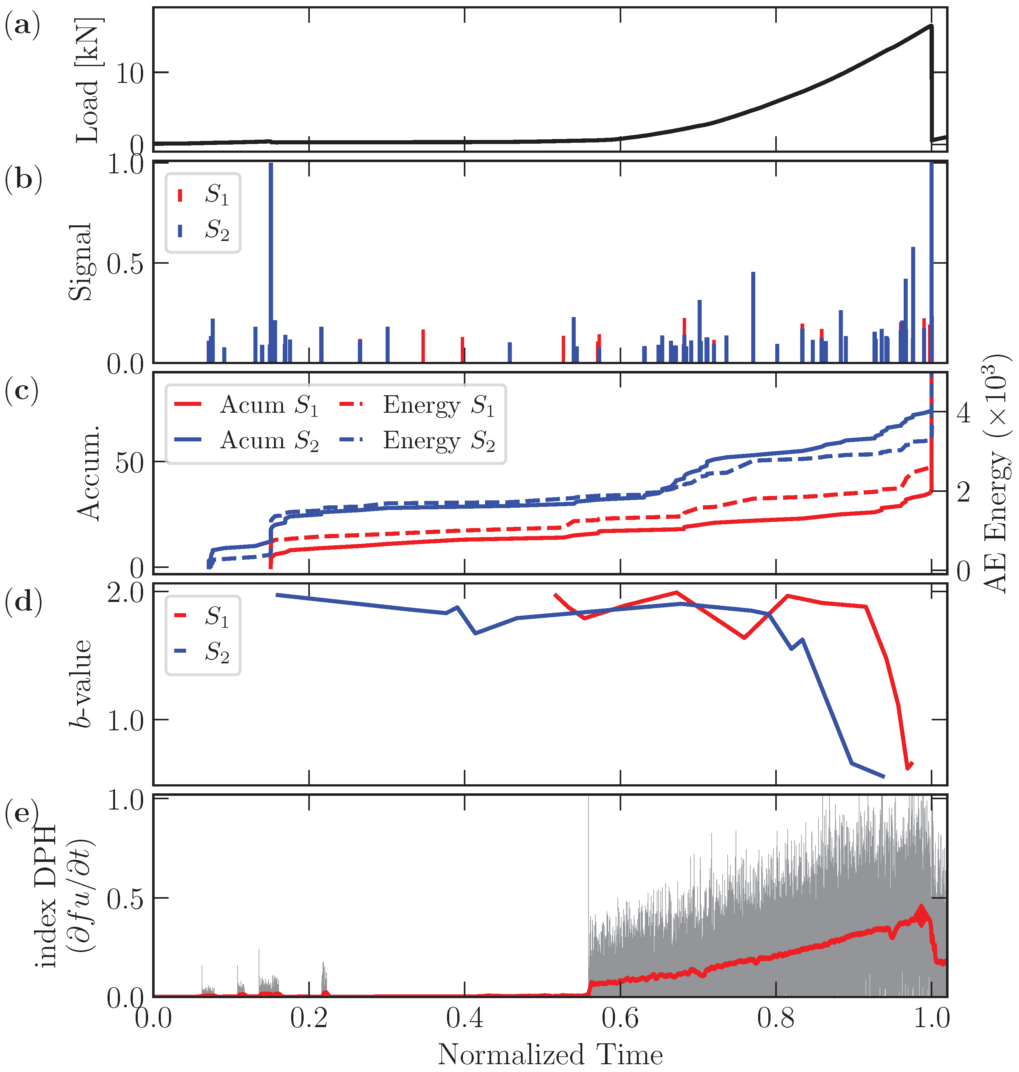
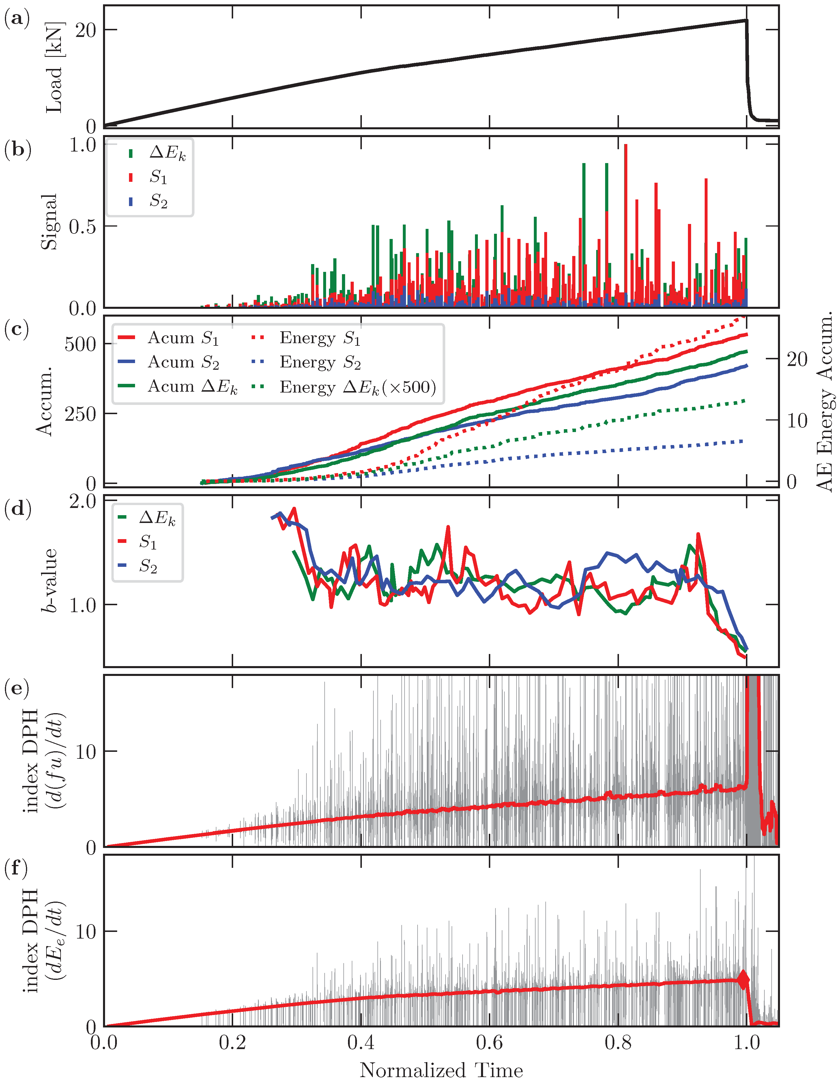
In the present work, four experimental tests were carried out; the specimens were named 1, 2, 3, and 4. The test using specimen 1 was discarded. In all tests, the load and displacement were captured. Additionally, in the test using specimen 4, the acoustic emission data were recorded and the results are plotted in Figure 7. All plots use normalized time, , where is the time when the load reaches 100% of its peak value.
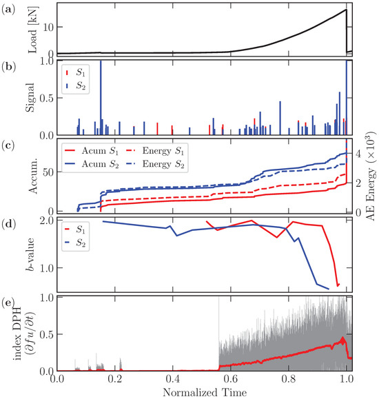
Figure 7.
Results for specimen 4 in terms of (a) load, (b) signal distribution, (c) the accumulated number of signals and signal energy, (d) the b-value, and (e) DPH index evolution. The horizontal axis is normalized time ().
In Figure 7, for specimen 4, the load vs. normalized time, signal amplitudes, accumulated signals, and AE energy are plotted. The b-value and DPH index evolution are presented for the information captured with sensor 1 and sensor 2, which were positioned as indicated in Figure 5c.
The following are observations about Figure 7:
- (i)
- (ii)
- The AE signals from sensors 1 and 2 are presented in Figure 7b. Note the high activity recorded at sensor 2 around the normalized time 0.15, which is due to the movement of the support, which is indicated by label 3 in Figure 5a. Furthermore, more AE emissions can be observed from sensor 2 (, right side) than from sensor 1 (, left side). This information is consistent with the final configuration presented in Figure 8c, where it is evident that the damage is concentrated on the right side of the specimen.
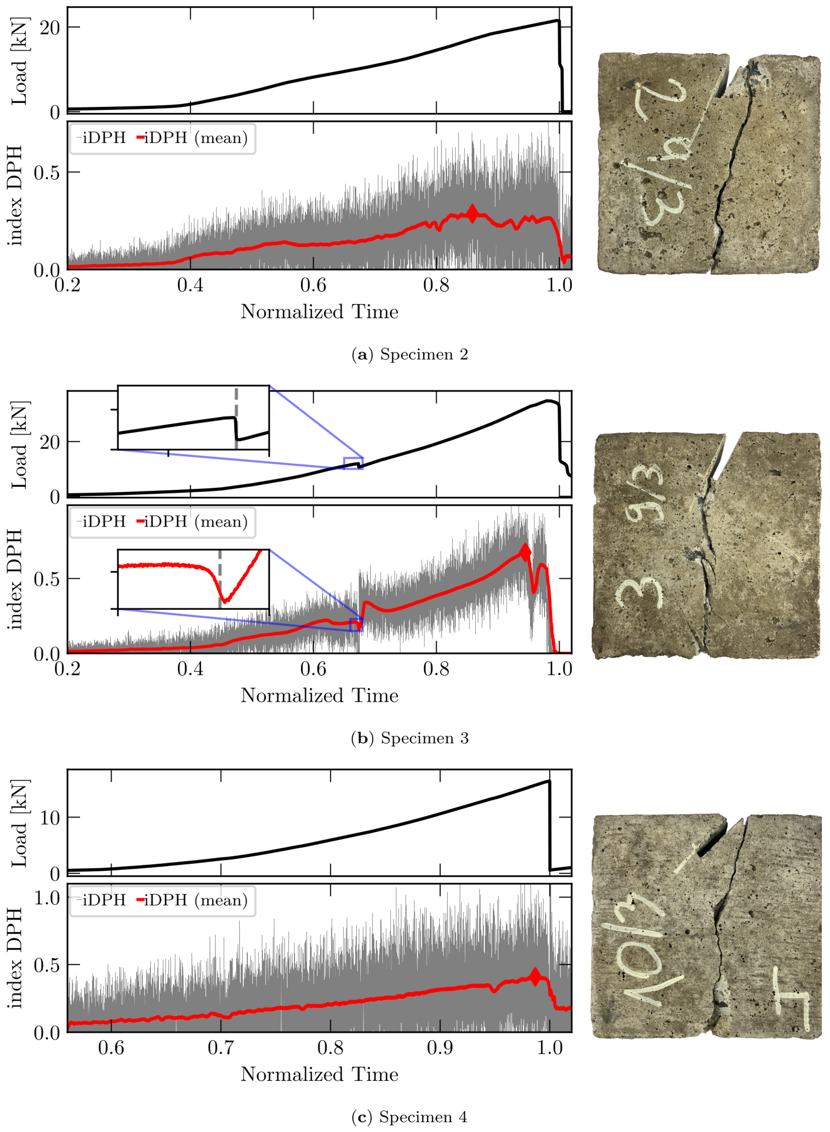
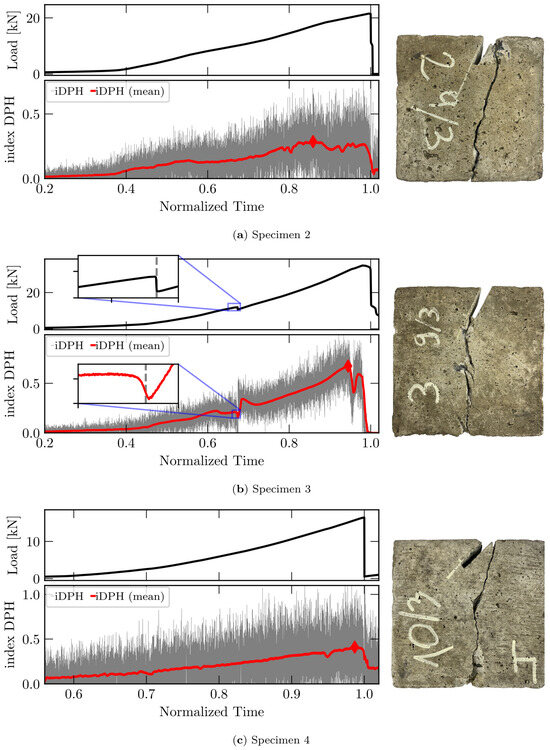 Figure 8. The results for (a) specimen 2, (b) specimen 3, and (c) specimen 4 in terms of the load and DPH index evolution vs. normalized time. The final configurations are also presented.
 - (iii)
- (iv)
- The evolution of the b-value is presented in Figure 7d. Note that both sensors indicate a drop in the b-value only at the end of the test when a collapse is expected. At , the b-value does not change due to the movement of the supports previously mentioned.
- (v)
- The evolution of the DPH index is presented in dark gray in Figure 7e. The moving average carried out in a window of 175 values is indicated in red in the same figure, and a red diamond indicates the maximum value of the DPH index. This value, as discussed in [26], can be considered a complementary precursor to collapse when an acoustic emission test is carried out. Note that, in the experimental case, the reaction load of the support (indicated by label 3 in Figure 5a) times the prescribed displacement is considered a measure of elastic energy, and from this value the derivative is calculated.
- (vi)
- Considering the methodology adopted by [26] and that which was previously described for determining a measure of elastic energy in an experimental test, it is possible to see an abrupt increase in the DPH index at . This is further evidence that the support cannot fix the specimen correctly before .
The load and DPH index vs. normalized time are presented in Figure 8, and the final configuration obtained from each test is also indicated. This information is presented for all tests performed for specimens 2, 3, and 4.
The following observations can be made about Figure 8:
- (i)
- The initial interval before the upper support actually solicited the specimen () was removed from the results presented for specimen 4 in Figure 8.
- (ii)
- The DPH index in all cases is presented in a dark gray color, and the moving average using 175 points is presented as a red line.
- (iii)
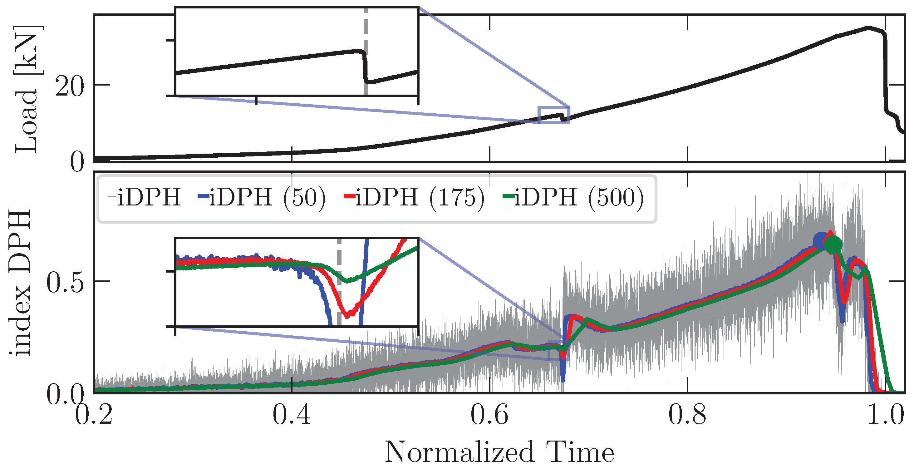
- Specimen 3 shows a final configuration different from specimens 2 and 4; this is also evidenced by the load and DPH index evolution. The local failure that appears in , when viewed in terms of DPH index evolution, shows that, before the local minimum appears, a smooth local maximum occurs, as evidenced by the detail presented in Figure 8b. This behavior is also investigated in Figure 9, where the sensibility of the number of data used to make the moving average is investigated.
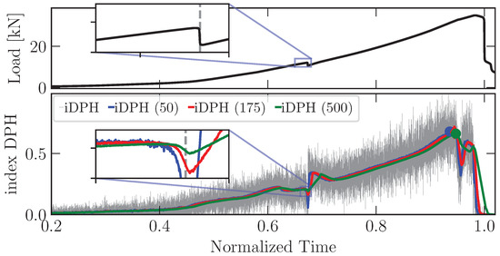 Figure 9. Study of the sensibility of the data window used in the moving average carried out for test 3. A window of 175 values is considered sufficient to obtain a clear evolution of the DPH index.
 - (iv)
- In all the tests, the maximum value of the DPH index appears close to the failure, and the local maximum also indicates some local failure during the test.
Figure 9 shows the sensibility of the window average on the evolution of the DPH index for the test with specimen 3. Windows of 50, 175, and 500 values were analyzed to obtain the moving average. The maximum values are indicated by markers. It is evident that a window of 175 values is enough to present a clear evolution of this index during the tests.
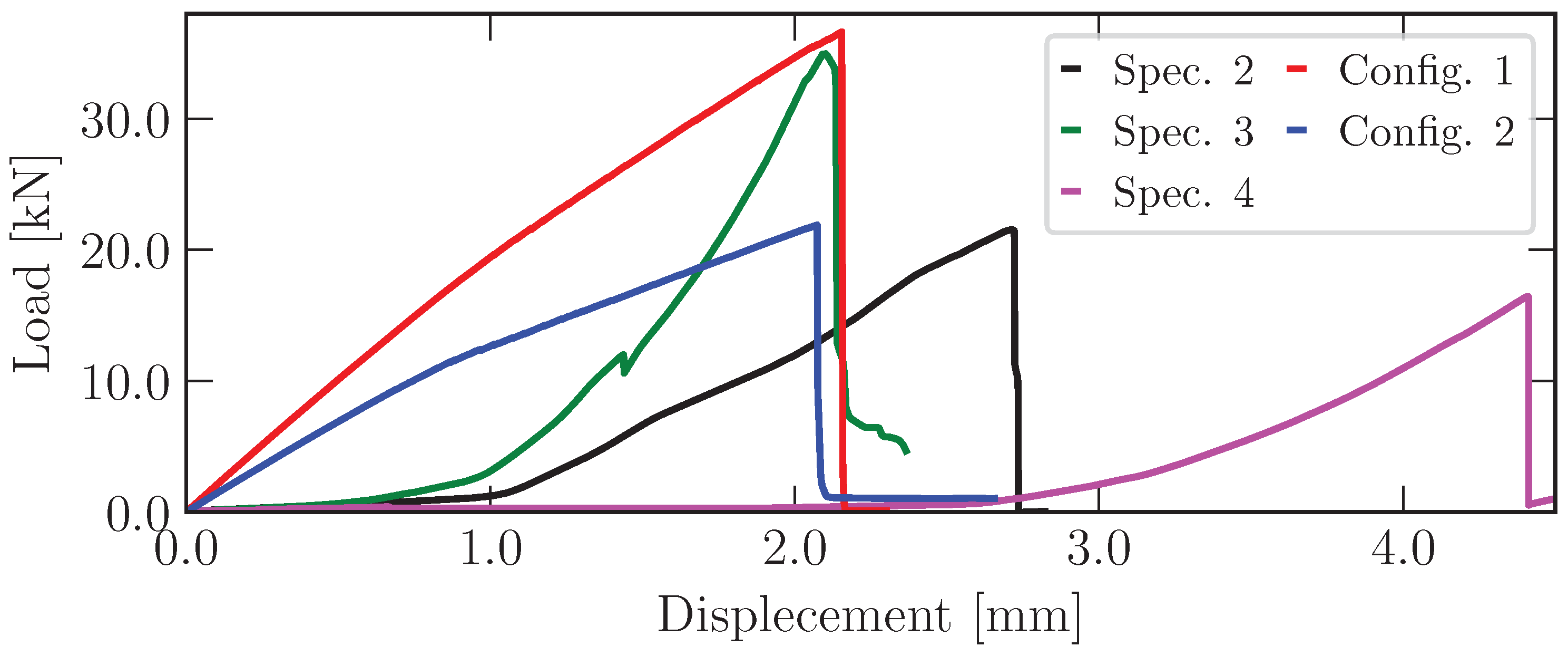
Finally, in Figure 10, the experimental results obtained in the tests for specimens 2, 3, and 4 are presented in terms of load vs. displacement. The excessive flexibility and lack of control in the supports with labels 2 and 3 in Figure 5a create different responses in the tests performed. In addition, the simulation for both configurations, analyzed in detail in the next section, is presented in the same domain.
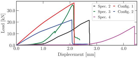
Figure 10.
The load vs. displacement for the experimental test and both simulations performed with the peridynamic model.
Notice that simulations were not performed only to adjust specific experimental tests but also to create similar configurations for the specimens tested.
5.2. Simulations Results
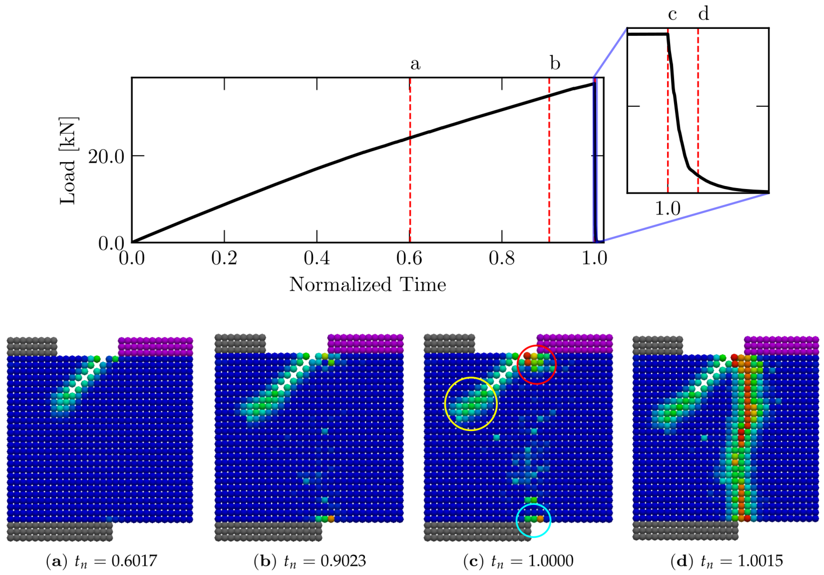
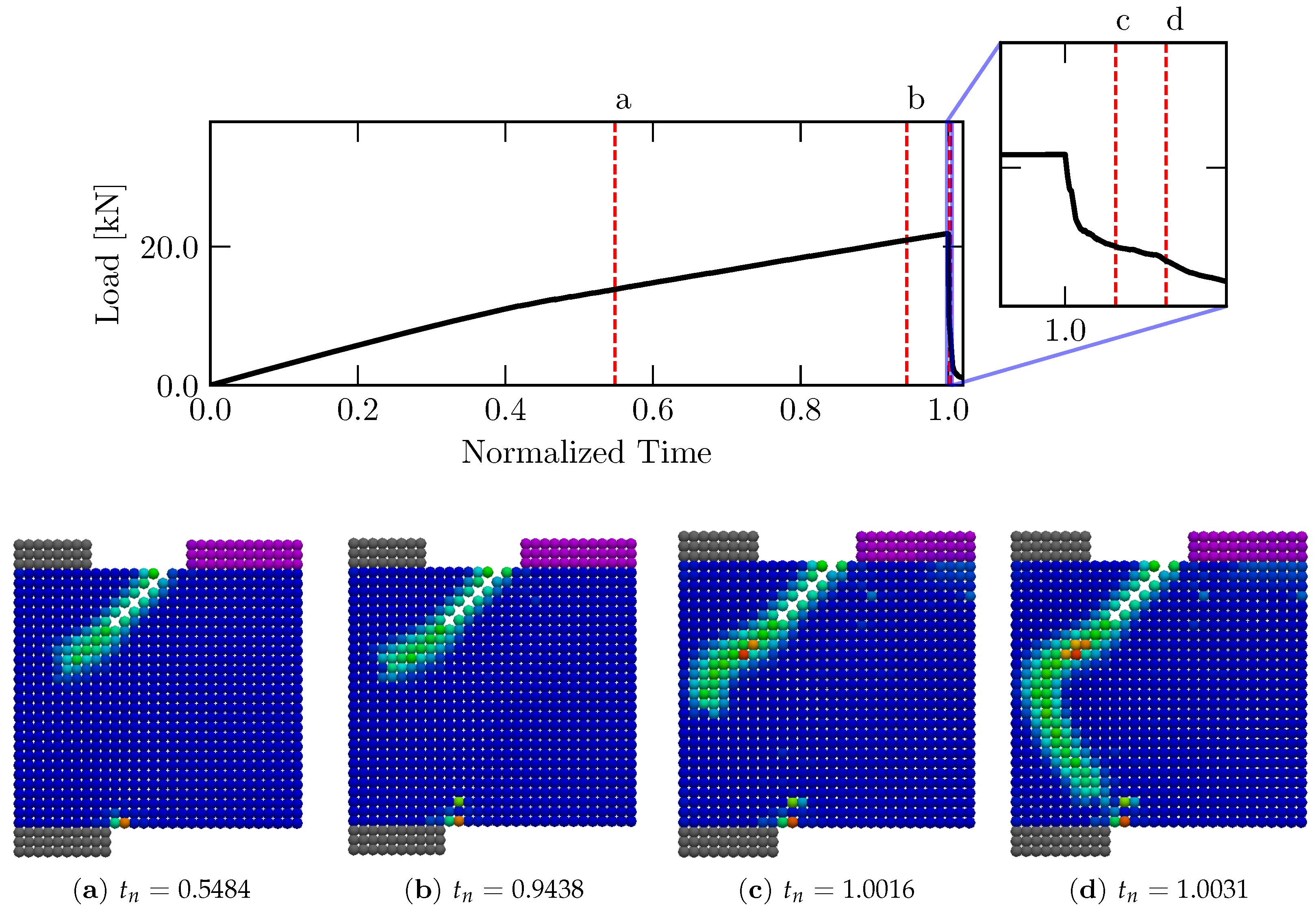
The results obtained from the two configurations described in Figure 6 are presented below. As in the experimental results, all plots use normalized time, , where is the time when the load reaches 100% of its peak value. In Figure 11, the partial configurations during the simulation are presented for Config. 1. At the top of Figure 11, the position of each configuration for load vs. normalized time is presented, and in Figure 11a–d the different configurations obtained during the simulation are shown.
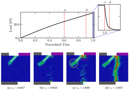
Figure 11.
Partial configuration for the Config. 1 simulation. The graph above is load vs. normalized time, along with the instant where the pictures were taken. The graphs below are the partial configurations at given instants and the final configuration of the damage.
Notice that, during the simulation, three sources of damage appear, indicated (in Figure 11c) by yellow (i), red (ii), and cyan (iii) circles. Notice that failure mechanisms (ii) and (iii) dominate the failure configuration only at the end of the process, as can be seen in Figure 11c,d.
Figure 12 presents the same organization as Figure 11 but is referred to as Config. 2; here, see that there are two clear sources of failure that are in competition, indicated by the yellow (i) and cyan (ii) circles in Figure 12a. Finally, the mechanism (i) leads to the final fracture configuration, but this definition happens only at the end of the process, as can be seen in Figure 12c,d.
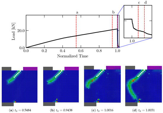
Figure 12.
Partial configuration for the Config. 2 simulation. The graph above is the load vs. normalized time, along with the instant where the pictures were taken. The graphs below are the partial configurations at given instants and the final configuration of the damage.
In addition, notice that diffuse damage occurs in the contact surface between the specimen and the upper support, indicated by a green box in Figure 12c.
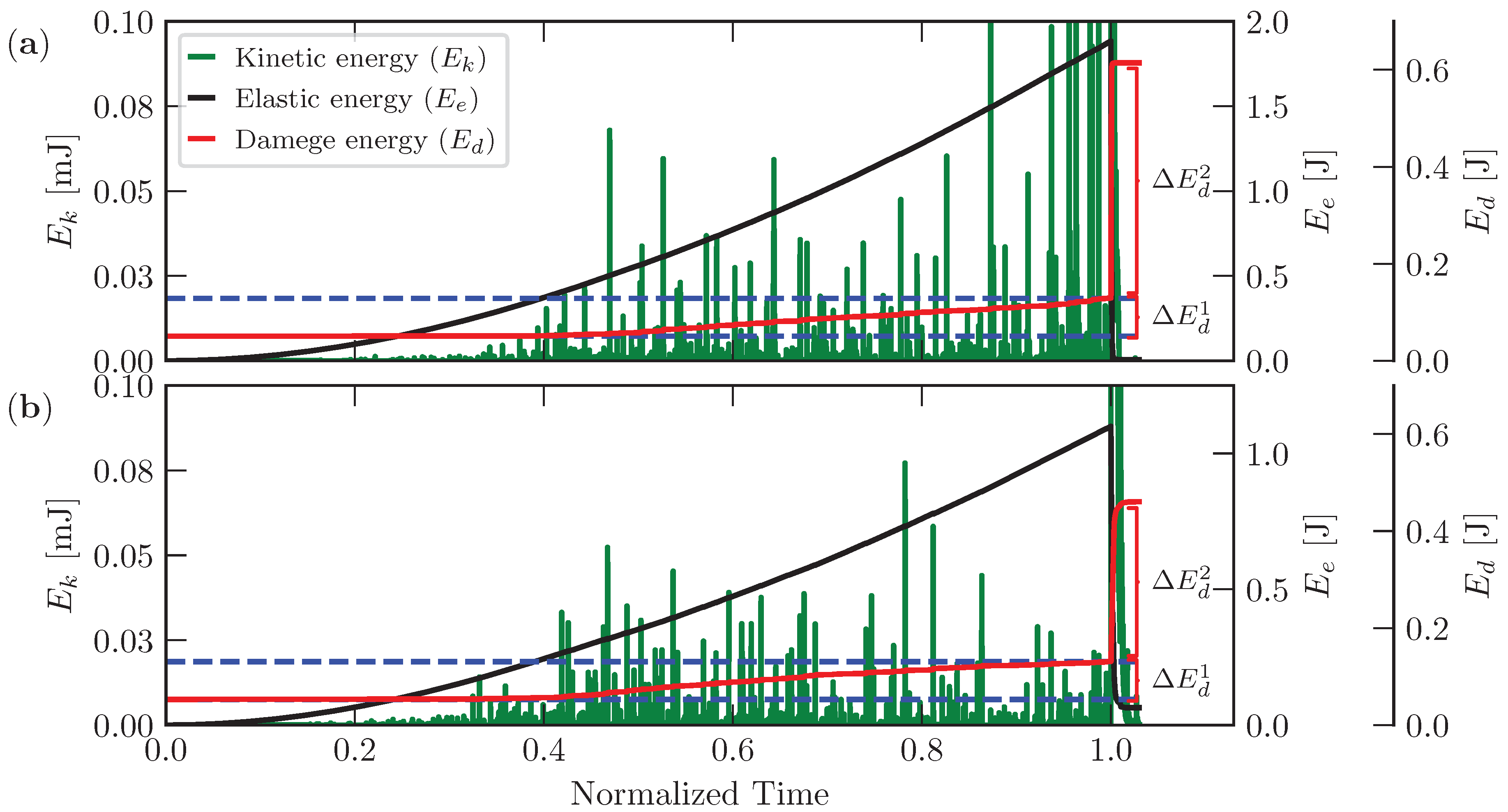
In Figure 13, the energy balance for Config. 1 and Config. 2 simulated using the peridynamic approach is presented. With the aim of facilitating a comparison, the three kinds of energy are plotted at different scales. The following can be seen in this figure:
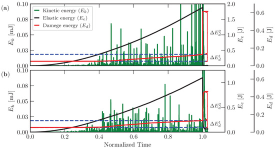
Figure 13.
Energy balance obtained using the peridynamic simulations: (a) Config. 1; and (b) Config. 2.
- (i)
- Damage energy does not begin at zero because when a pre-notch is created (as shown in Figure 6c) the peridynamic model computes the damage energy of each bond deactivated to create this pre-notch.
- (ii)
- The abrupt drop in damage energy that is wasted when the final failure happens is called , and the value of energy dissipated smoothly up to reach the eminence of the final fracture is called . The inspection of these two values confirms that Config. 1 presents more brittle behavior than Config. 2, dissipating practically the same quantity of energy up to arriving at the final configuration ( value) but presenting a sharper decrease in terms of for Config. 1 ( ) than that of Config. 2 ( ).
- (iii)
- Reinforcing the observation (ii) that the increase in elastic energy is more accentuated in Config. 1 than in Config. 2, there is an indication that more elastic energy () is available to produce a brittle failure in Config. 1 ( ) than in Config. 2 ( ).
- (iv)
- The kinetic energy evaluation during the simulation shows a sensible increase after the specimens begin to show a smooth increase in the dissipated energy close to for both configurations. In addition, fluctuations increase at the end of the simulations when the final failure happens, and notice that in Config. 1 these fluctuations are higher than in Config. 2, which is in agreement with the fact that Config. 1 presents increased brittle behavior.
Acoustic emission tests were also simulated in Config. 1 and Config. 2. Accelerations perpendicular to the surface placed in the same positions as sensor 1 and sensor 2 were captured, and these were considered AE signals.
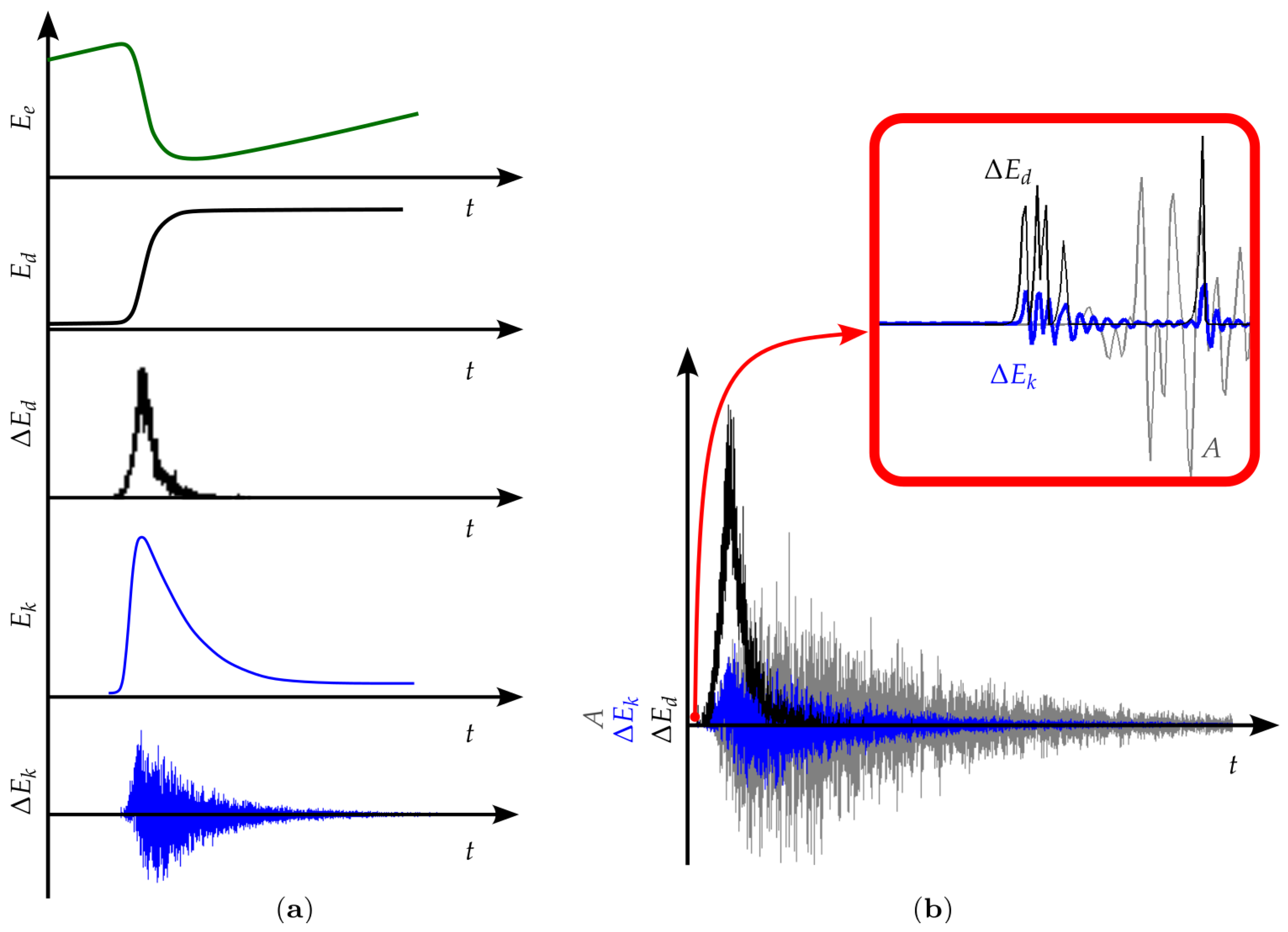
The temporal derivative of the kinetic energy computed with the model , here called , will have the same acoustic emission signal distribution pattern with time, as was pointed out in [34]. The difference between and the signal distribution obtained with each sensor is that is computed using the kinetic energy measure in the model. This avoids the loss or distortion of information due to the wave traveling in the solid from the event source to the AE device.
In Figure 14a, energy balance details of when an event happens are presented, where the elastic, dissipated, and kinetic energies change during the event. In the same Figure, the derivative of the dissipated energy, , and the kinetic energy, , are presented. It is easy to perceive that the pattern of is like the typical AE signal. In [35,36], the indirect link between the energy dissipated by the event and the AE signal is discussed. In this discussion, it remains clear that the AE signal relates to the energy that makes noise; that is, the kinetic energy creates an indirect relation between the fall in the elastic energy and the dissipated energy.
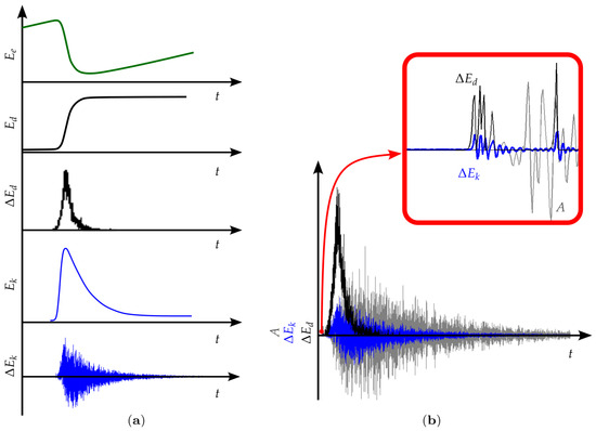
Figure 14.
The link between the information computed during the energy balance and its relationship with the acoustic emission signal. (a) The energy balance for a typical event during a process where the variation in is presented. In the same plot, the derivatives of the dissipated energy, , and kinetic energy, , are shown. (b) The superposition of and the EA signal are illustrated. The beginning of the curves is presented to demonstrate the delay between A, , and .
The signals captured with the device, , , and , are presented in Figure 14b. The similarity between the signature and is evident. In the details of the same Figure 14b, the delay between A(t) and , , is indicated. is computed directly from the model energy balance and is then manifested when the event happens; the acoustic emission signal () has a delay in comparison with because the signal is captured in the AE device after the elastic wave arrives in the sensor.
The possibility to compute as an alternative measure of is only possible in the simulation, but comparing the numerical and could obtain complementary information to interpret the AE experimental test.
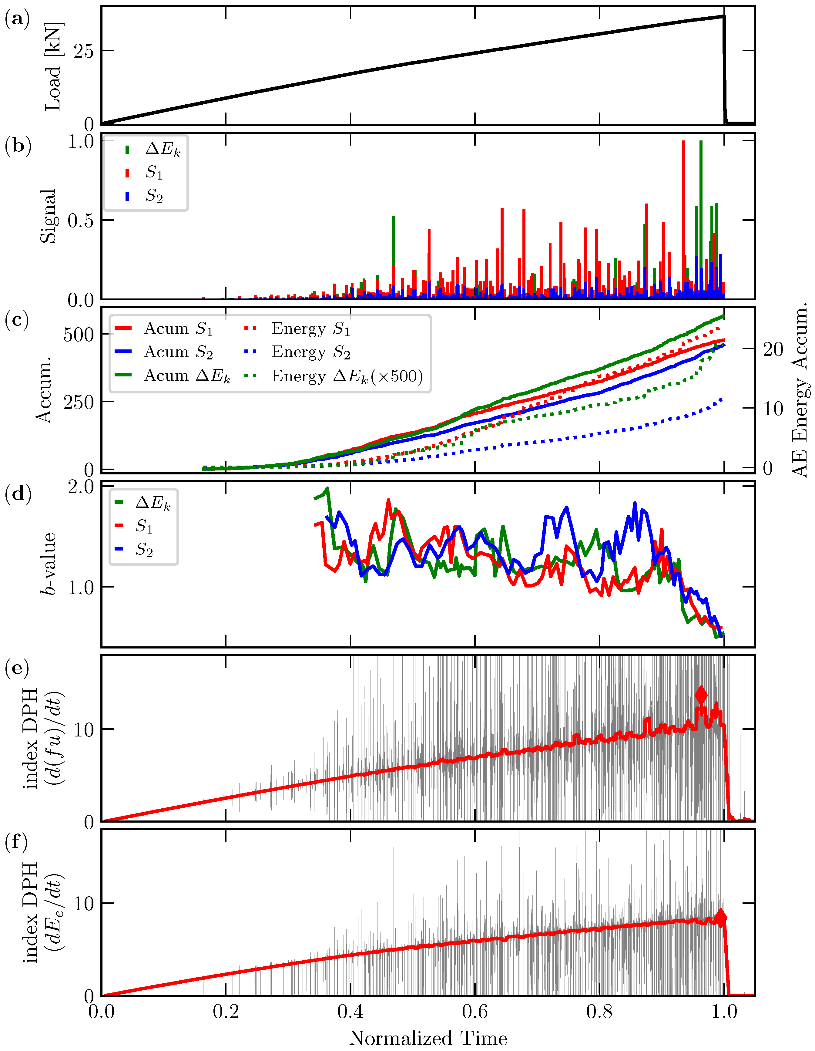
In Figure 15 and Figure 16, the results related to the simulation of the AE tests are presented for Config. 1 and Config. 2. All parameters are plotted vs. normalized time. In (a), the global load is presented. In (b), the AE signal obtained for sensor 1 and sensor 2 (placed as indicated in Figure 5c) is shown. In (c), the accumulated number of signals (Acum and Acum ) and the number of events measured from are plotted. In the same plot, information on accumulated AE energy is presented. In (d), b-value evolution is computed using the acoustic emission signal for sensors 1 and 2, and the b-value is computed using the information, which is also presented. In (e), DPH index evolution, which was computed using the product of the displacement prescribed times the correspondent reaction force (), is illustrated. Finally, in (f), DPH index evolution, which was computed using the elastic energy obtained from the overall energy balance of the simulation (), is depicted.
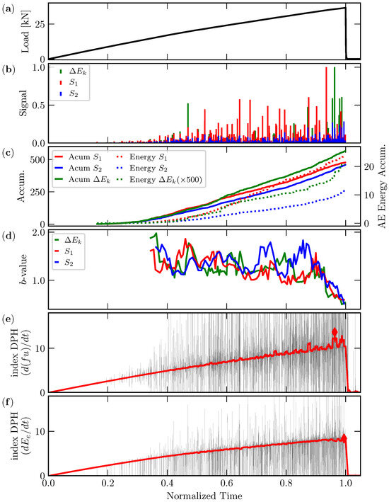
Figure 15.
Numerical results for Config. 1. (a) Load vs. normalized time; (b) temporal distribution of the amplitude signals for sensor 1 (left device) and sensor 2 (right device) and the signal computed from the kinetic energy measured during the simulation (). (c) The accumulated number of signals for both sensors, and the accumulated energy magnitudes, measured using the RILEM methodology; the same information was computed from , an alternative measure of AE information. (d) b-value evolution obtained using sensor 1, sensor 2, and . (e) DPH index evolution, obtained using the methodology of [26]. (f) DPH index evolution, computed using the elastic energy in the simulation.
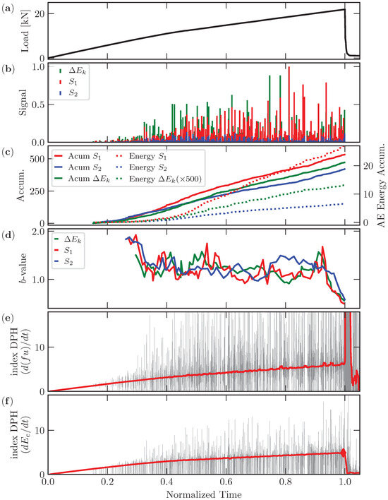
Figure 16.
Numerical results for Config. 2. (a) Load vs. normalized time; (b) temporal distribution of the amplitude signals for sensor 1 (left device) and sensor 2 (right device) and the signal computed from the kinetic energy measured during the simulation (). (c) The accumulated number of signals for both sensors and the accumulated energy magnitudes, measured using the RILEM methodology; the same information was computed from , an alternative measure of AE information. (d) b-value evolution obtained using sensor 1, sensor 2, and . (e) DPH index evolution, obtained using the methodology of [26]. (f) DPH index evolution, computed using elastic energy in the simulation.
In the analysis of these figures, we make the following observations:
- (i)
- For Config. 1, it is evidenced that, in Figure 15b, sensor 1 recorded more signal activity than sensor 2 until . After this time, the same activity in both sensors is observed. This fact is coherent with the evolution of the configurations presented in Figure 11a,b; until , high AE activity comes from the pressure head. This source is close to sensor 1. This tendency changes after , when the failure mechanism changes, as is depicted in Figure 11c,d. In the second mechanism, the source of AE activity is close to sensor 2.
- (ii)
- On the other hand, sensor 1 registers more AE activity during all of the simulations in Config. 2, as shown in Figure 16b, and, in this case, this fact is coherent with the configuration presented in Figure 12a–d, which show the crack tip as the main failure source of AE activity during all simulations.
- (iii)
- In Figure 15b and Figure 16b, it is interesting to compare the signal obtained from the two sensors and the equivalent information obtained from . In this comparison, it is possible to measure how the travel between the event source and the device modified the acoustic emission signal captured. The simulation of this situation might suggest placing the AE sensor in a better position in the experimental test. Particularly, in the present case, sensor 1 is better positioned than sensor 2. In general, it will be possible to determine if the combination of specimen geometry, boundary condition, and damage distribution can help identify the best position for the AE sensors.
- (iv)
- In Figure 15c and Figure 16c, the number of accumulated signals and the change in signal energy during the simulation are presented. In both configurations, the results in terms of the number of signals and energy indicate higher activity registered in sensor 1 until the final part of the simulation in Config. 1 and during all the simulations in Config. 2. The measure of the accumulated number of events and the accumulated energy computed from are coherent with the results obtained from the signal information obtained with the AE sensors.
- (v)
- (vi)
- The DPH index presented in Figure 15e,f shows a maximum value before arriving at the failure in both cases. Notice that obtaining the DPH index directly from the elastic energy or from a measure of the elastic energy (reaction support times the support displacement) indicates the same tendency.
6. Conclusions
In the present work, a concrete prism with pre-notching was analyzed. Three tests were performed, but the flexibility of the support produced uncontrolled boundary conditions. AE information was captured in one of the tests, and two similar simulations using a peridynamic model that considered different boundary conditions were carried out. In the numerical models, an AE test was simulated. In the experimental test and numerical model, the evolution of the DPH index was also computed, which is a parameter that can be used to gather complementary information regarding the AE test.
We draw the following conclusions:
- The three tests carried out showed high dependency on the flexibility of the support, with the three tests presenting quite different displacements and final configurations.
- A strong dependence on boundary conditions was also seen in the simulation results using the peridynamic model.
- The acoustic emission information obtained in the tests presented coherency, and the results allowed for explanations regarding the damage process analyzed.
- The evaluation of the DPH index for all the specimens tested and the simulations demonstrated the potential of this index to indicate a maximum value close to a local or global collapse. In all the cases analyzed, the value of the DPH index presented a maximum before the collapse occurs. This parameter could provide complementary information in AE analysis.
- The simulation of the two configurations indicated the potential of the peridynamic model to represent an AE test and the possibility to obtain information that aids AE experimental testing.
- Specifically in the simulations, the possibility of comparing the signal measured with the device and an alternative measure called is interesting; this information could be used to perceive distortions in the waves that travel between the signal event source and the signal captured by the device. This analysis could be used to define the best position for the AE device in the experimental test.
Finally, we consider that the main goal of the present study was accomplished; the performance of the DPH index and the numerical simulation of acoustic emission using a peridynamic model could be a good alternative to help with the interpretation of AE information obtained in such tests.
Author Contributions
Conceptualization, W.R.A., B.N.R.T., I.I. and G.L.; methodology, W.R.A., B.N.R.T., I.I. and G.L.; software, W.R.A. and B.N.R.T.; validation, W.R.A. and B.N.R.T.; formal analysis, W.R.A., B.N.R.T. and I.I.; investigation, W.R.A., B.N.R.T. and I.I.; resources, I.I. and G.L.; data curation, I.I. and G.L.; writing—original draft preparation, W.R.A., B.N.R.T., G.B. and I.I.; writing—review and editing, W.R.A., B.N.R.T., G.B., I.I. and G.L.; visualization, B.N.R.T.; supervision, G.L. and I.I.; project administration, I.I.; funding acquisition, I.I. and G.L. All authors have read and agreed to the published version of the manuscript.
Funding
This research was funded by the Brazilian National Council for Scientific and Technological Development (CNPq, Brazil), the Coordination for the Improvement of Higher Education Personnel (CAPES-Brazil) and the sponsorship guaranteed with basic research funds was provided by Politecnico di Torino.
Institutional Review Board Statement
Not applicable.
Informed Consent Statement
Not applicable.
Data Availability Statement
Data are contained within the article.
Conflicts of Interest
The authors declare no conflicts of interest.
Abbreviations
The following abbreviations are used in this manuscript:
| AE | Acoustic emission |
| DPH | Dȩbski–Pradhan–Hansen |
| GR | Gutenberg–Richter |
References
- Kachanov, L.M. Introduction to Continuum Damage Mechanics. In Mechanics of Elastic Stability; Springer: Dordrecht, The Netherlands, 1986; Volume 10. [Google Scholar] [CrossRef]
- Park, T.; Ahmed, B.; Voyiadjis, G.Z. A review of continuum damage and plasticity in concrete: Part I—Theoretical framework. Int. J. Damage Mech. 2022, 31, 901–954. [Google Scholar] [CrossRef]
- Voyiadjis, G.Z.; Ahmed, B.; Park, T. A review of continuum damage and plasticity in concrete: Part II—Numerical framework. Int. J. Damage Mech. 2022, 31, 762–794. [Google Scholar] [CrossRef]
- Zhang, K.; Badeddline, H.; Yue, Z.; Hfaiedh, N.; Saanouni, K.; Liu, J. Failure prediction of magnesium alloys based on improved CDM model. Int. J. Solids Struct. 2021, 217–218, 155–177. [Google Scholar] [CrossRef]
- Krajcinovic, D. Damage Mechanics; North-Holland series in applied mathematic and mechanics, 41; Elsevier: Amsterdam, The Netherlands; New York, NY, USA, 1996; ISBN 978-0-444-82349-6. [Google Scholar]
- Mastilovic, S.; Rinaldi, A. Two-Dimensional Discrete Damage Models: Discrete Element Methods, Particle Models, and Fractal Theories. In Handbook Of Damage Mechanics; Springer: New York, NY, USA, 2013; pp. 1–27. [Google Scholar] [CrossRef]
- Jenabidehkordi, A. Computational methods for fracture in rock: A review and recent advances. Front. Struct. Civ. Eng. 2018, 13, 273–287. [Google Scholar] [CrossRef]
- Silling, S. Reformulation of elasticity theory for discontinuities and long-range forces. J. Mech. Phys. Solids 2000, 48, 175–209. [Google Scholar] [CrossRef]
- Silling, S.; Askari, E. A meshfree method based on the peridynamic model of solid mechanics. Comput. Struct. 2005, 83, 1526–1535. [Google Scholar] [CrossRef]
- Bobaru, F.; Foster, J.; Geubelle, P.; Silling, S. Handbook of Peridynamic Modeling; Taylor & Francis: Boca Raton, FL, USA, 2015. [Google Scholar]
- Huang, K. Statistical Mechanics, 2nd ed.; Wiley: New York, NY, USA, 1987. [Google Scholar]
- Biswas, S.; Ray, P.; Chakrabarti, B.K. Statistical Physics of Fracture, Breakdown, and Earthquake: Effects of Disorder and Heterogeneity; John Wiley & Sons: Weinheim, Germany, 2015. [Google Scholar]
- Kawamura, H.; Hatano, T.; Kato, N.; Biswas, S.; Chakrabarti, B.K. Statistical Physics of Fracture, Friction and Earthquake. Rev. Mod. Phys. 2012, 84, 839–884. [Google Scholar] [CrossRef]
- Rundle, J.B.; Turcotte, D.L.; Shcherbakov, R.; Klein, W.; Sammis, C. Statistical physics approach to understanding the multiscale dynamics of earthquake fault systems: Statistical physics of Earthquakes. Rev. Geophys. 2003, 41. [Google Scholar] [CrossRef]
- Hansen, A.; Hemmer, P.C.; Pradhan, S. The Fiber Bundle Model: Modeling Failure in Materials; Statistical Physics of Fracture and Breakdown; Wiley-VCH Verlag GmbH & Co. KGaA: Weinheim, Germany, 2015. [Google Scholar]
- Varotsos, P. Spatio-temporal complexity aspects on the interrelation between seismic electric signals and seismicity. Pr. Athens Acad 2001, 76, 294. [Google Scholar]
- Wilson, K.G. Problems in Physics with many Scales of Length. Sci. Am. 1979, 241, 158–179. [Google Scholar] [CrossRef]
- Richter, C.F. Elementary Seismology; W. H. Freeman and Company: New York, NY, USA; Bailey Bros. & Swinfen Ltd.: London, UK, 1958; Volume 2. [Google Scholar]
- Sethna, J.; Dahmen, K.; Myers, C. Crackling noise. Nature 2001, 410, 242–250. [Google Scholar] [CrossRef] [PubMed]
- Grosse, C.; Ohtsu, M. (Eds.) Acoustic Emission Testing; Springer: Berlin/Heidelberg, Germany, 2008. [Google Scholar] [CrossRef]
- Carpinteri, A.; Lacidogna, G.; Puzzi, S. From criticality to final collapse: Evolution of the “b-value” from 1.5 to 1.0. Chaos Solitons Fractals 2009, 41, 843–853. [Google Scholar] [CrossRef]
- Aki, K. Scaling Law of Seismic Spectrum. J. Geophys. Res. 1967, 72, 1217–1231. [Google Scholar] [CrossRef]
- Carpinteri, A.; Lacidogna, G.; Pugno, N. Richter’s laws at the laboratory scale interpreted by acoustic emission. Mag. Concr. Res. 2006, 58, 619–625. [Google Scholar] [CrossRef]
- Varotsos, P.A.; Sarlis, N.V.; Skordas, E.S. Natural Time Analysis: The New View of Time; Springer: Berlin/Heidelberg, Germany, 2011. [Google Scholar] [CrossRef]
- Dȩbski, W.; Pradhan, S.; Hansen, A. Criterion for Imminent Failure During Loading—Discrete Element Method Analysis. Front. Phys. 2021, 9, 675309. [Google Scholar] [CrossRef]
- Rojo Tanzi, B.N.; Sobczyk, M.; Iturrioz, I.; Lacidogna, G. Damage Evolution in Quasi-Brittle Materials: Experimental Analysis by AE and Numerical Simulation. Appl. Sci. 2023, 13, 10947. [Google Scholar] [CrossRef]
- Puglia, V.B.; Kosteski, L.E.; Riera, J.D.; Iturrioz, I. Random field generation of the material properties in the lattice discrete element method. J. Strain Anal. Eng. Des. 2019, 54, 236–246. [Google Scholar] [CrossRef]
- Shimadzu Corporation. AGS-X Plus: Instruction Manual; Shimadzu: Kyoto, Japan, 2012. [Google Scholar]
- Madenci, E.; Oterkus, E. Peridynamic Theory and Its Applications; Springer: Berlin/Heidelberg, Germany, 2014. [Google Scholar]
- Taylor, D. The theory of critical distances. Eng. Fract. Mech. 2008, 75, 1696–1705. [Google Scholar] [CrossRef]
- Bažant, Z.; Planas, J. Fracture and Size Effect in Concrete and Other Quasibrittle Materials; Routledge: London, UK, 2019; Volum 3. [Google Scholar] [CrossRef]
- Birck, G.; Iturrioz, I.; Lacidogna, G.; Carpinteri, A. Damage process in heterogeneous materials analyzed by a lattice model simulation. Eng. Fail. Anal. 2016, 70, 157–176. [Google Scholar] [CrossRef]
- Rossi Cabral, N.; Invaldi, M.; Barrios D’Ambra, R.; Iturrioz, I. An alternative bilinear peridynamic model to simulate the damage process in quasi-brittle materials. Eng. Fract. Mech. 2019, 216, 106494. [Google Scholar] [CrossRef]
- Iturrioz, I.; Lacidogna, G.; Carpinteri, A. Acoustic emission detection in concrete specimens: Experimental analysis and lattice model simulations. Int. J. Damage Mech. 2014, 23, 327–358. [Google Scholar] [CrossRef]
- Carpinteri, A.; Lacidogna, G.; Corrado, M.; Di Battista, E. Cracking and crackling in concrete-like materials: A dynamic energy balance. Eng. Fract. Mech. 2016, 155, 130–144. [Google Scholar] [CrossRef]
- Rojo Tanzi, B.N.; Birck, G.; Sobczyk, M.; Iturrioz, I.; Lacidogna, G. Truss-like Discrete Element Method Applied to Damage Process Simulation in Quasi-Brittle Materials. Appl. Sci. 2023, 13, 5119. [Google Scholar] [CrossRef]

Disclaimer/Publisher’s Note: The statements, opinions and data contained in all publications are solely those of the individual author(s) and contributor(s) and not of MDPI and/or the editor(s). MDPI and/or the editor(s) disclaim responsibility for any injury to people or property resulting from any ideas, methods, instructions or products referred to in the content. |
© 2024 by the authors. Licensee MDPI, Basel, Switzerland. This article is an open access article distributed under the terms and conditions of the Creative Commons Attribution (CC BY) license (https://creativecommons.org/licenses/by/4.0/).