An Analysis of the 2008 M_s 8.0 Wenchuan Earthquake’s Aftershock Activity

Abstract

We investigated the magnitude–frequency relationship and decay pattern of an aftershock sequence using data from the 2008 Wenchuan earthquake. We analyzed the spatial variations in aftershock activity parameters b and p. The calculated b-value of the aftershock sequence is 0.89 ± 0.02, which is relatively small, probably owing to the absence of small earthquakes in the aftershock catalog. The p-value, indicating the decay rate of aftershock activity, is 1.05 ± 0.02, which is normal. The decay pattern of the Wenchuan aftershock sequence agrees well with the modified Omori law. The b-value of the aftershock sequence mainly spatially varies between 0.6 and 1.2, and the p-value varies between 0.6 and 1.8. Although the physical significance of the spatial variations in b- and p-values has not been clearly defined, in this study, the physical significance of the b-value is mainly related to changes in stress, P-wave velocity, and the density of media in the earthquake area, and that in the p-value is associated with the fault slip amount during the mainshock; the b- and p-values show a strong linear correlation. After the mainshock, stress decreased and increased in areas with large and small b-values, respectively; the regions with large and small b-values were associated with low and high P-wave velocities, respectively. The subsurface media experienced relatively high and low apparent velocities in areas with small and large b-values, respectively. The amount of fault slip was small and large in regions with small and large p-values, respectively, exhibiting a linear correlation between the fault slip amount and p-value. The results indicate that the spatial variations in the b- and p-values were related to the physical properties of the media in the earthquake area and focal earthquake mechanism.

1. Introduction

The M8.0 earthquake in Wenchuan on 12 May 2008 caused extensive losses of both life and property. However, the occurrence of this earthquake provided abundant information for seismologists to study seismogenic mechanisms, the Earth’s crustal structure, and petrophysical properties. In particular, the large number of aftershocks occurring within a short period in a small area after the mainshock provided valuable basic information for studies of the source properties of the large earthquake and the characteristics of the aftershock activity. In recent years, scholars in China and abroad have increasingly paid attention to the characteristics of aftershock activities, establishing various statistical models focusing on the spatiotemporal patterns and intensity of the aftershocks [1,2,3,4,5]. The most famous models include the Gutenberg–Richter (G-R) law [1], which describes earthquake intensity, and the modified Omori law [2,3]. The method we use in this study calculates the goodness of fit between a power law fit to the data and the observed frequency–magnitude distribution as a function of a lower cutoff of the magnitude data [4], describing the decay pattern of aftershocks. For more than 20 years, ETAS models have been used to analyze seismic activity. Dynamic behavior has been widely used and developed, and the ETAS model is also considered as the benchmark model for seismic activity modeling [6,7,8]. By studying the magnitude–frequency relationship of aftershocks and their decay patterns, we can more thoroughly understand the characteristics of aftershock activities, which is valuable for predicting strong aftershocks and mitigating aftershock losses. In this study, we mainly investigated the features of the spatiotemporal variation in aftershock activities using the aftershock sequence of the Wenchuan earthquake based on the above two statistical models and discussed the relationship between the aftershock activity parameters, the focal mechanism of the earthquake, and the physical properties of the media in the earthquake area.

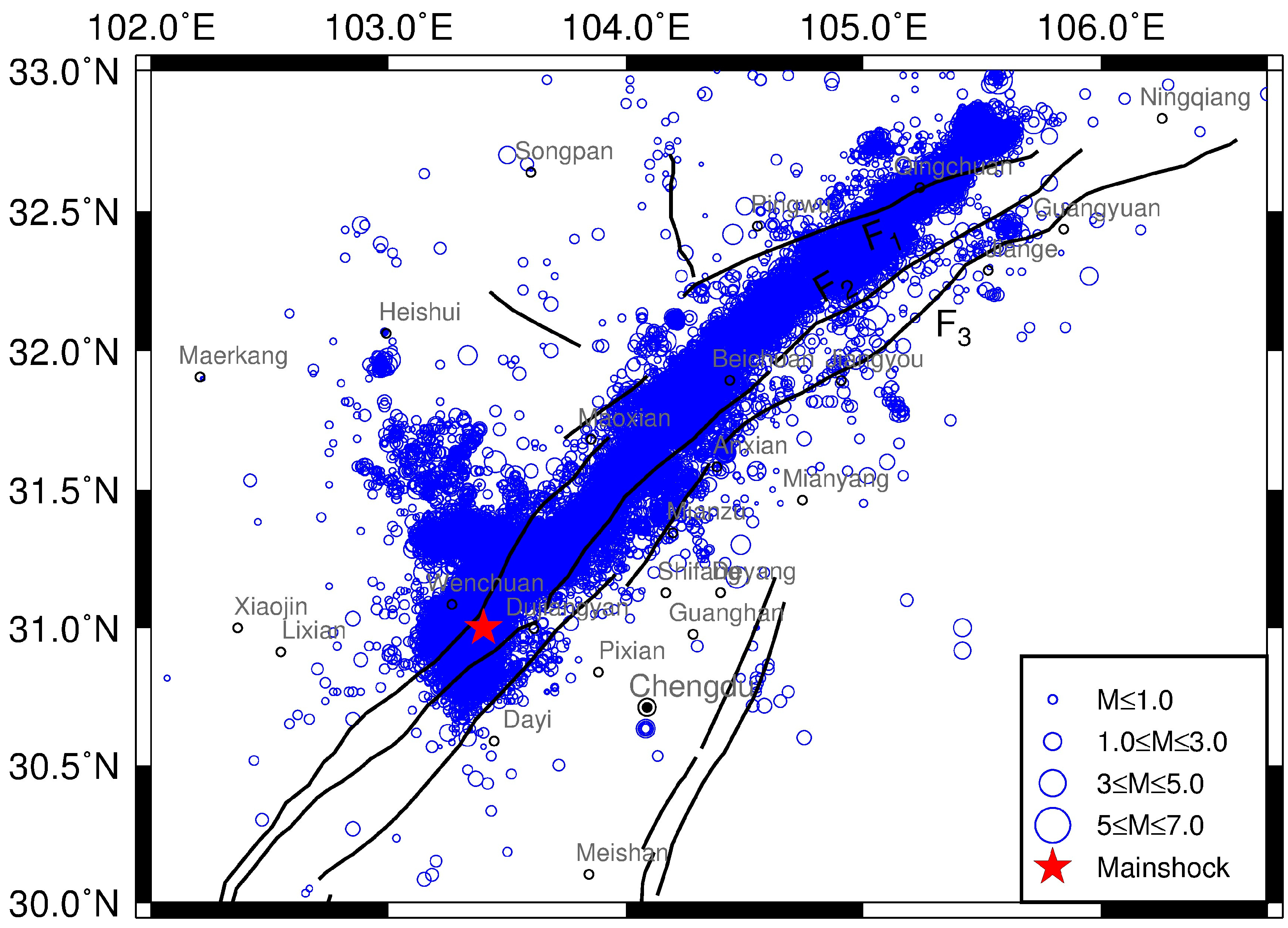
2. Data and Data Completeness

2.1. Data Sources

The aftershock catalog of the Wenchuan earthquake used in this study was retrieved from the Sichuan Provincial Seismological Bureau, and the location and magnitude of the aftershock events were determined using the Sichuan provincial seismic network (Figure 1). The applied aftershock catalog covers the period from 12 May 2008 to 29 December 2008.

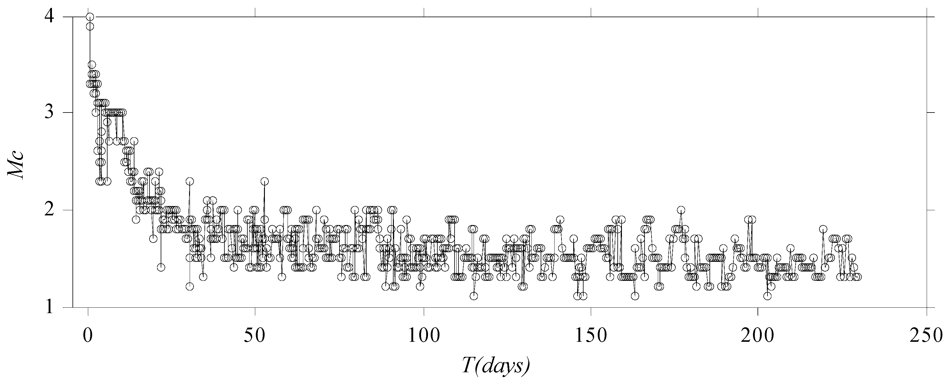
2.2. Completeness Analysis

Determining the initial completeness magnitude of the aftershock catalog M_c is crucial for studying aftershock activity as it affects the reliability of the study’s results. Wiemer and Wyss [4] proposed the following method to estimate the minimum completeness magnitude. Assume that the distribution of earthquake magnitudes conforms to the G-R law. Then, the smallest magnitude M_i is selected; the observed data with M ≥ M_i are fitted according to the G-R relationship so that the theoretical values for each magnitude interval can be determined using the fitted parameters. Finally, the absolute difference between the theoretical and observed values is obtained as follows:

$$R=(a,b,M_i)=100-\left[\frac{{\displaystyle \sum _{M_i}^{M_{\max }}|B_i-S_i|}}{{\displaystyle \sum _i{B}_i}}100\right]$$

(1)

where B_i and S_i are the observed and theoretical numbers of earthquakes in each magnitude interval, respectively. The value of M_i gradually increases, and M_i is considered the minimum complete magnitude M_c until R ≥ 95.

Using the above method, we explored the pattern of spatiotemporal variation in the minimum completeness magnitude. After an earthquake, seismic monitoring in the epicenter area inevitably strengthens, so the minimum completeness magnitude that can be monitored decreases over time. We investigated the temporal variation in the minimum complete magnitude M_c using a moving time window approach [9]. First, we estimated M_c using 200 aftershocks following the mainshock; then, we moved the window forward in time by 100 earthquakes to successively calculate M_c to obtain the pattern of the temporal variation in M_c (Figure 2). In Figure 2, M_c roughly exhibits an exponential decaying trend over time. In the first few hours after the mainshock, M_c fluctuated around a magnitude of 3.5 and then sharply dropped to approximately 2.5. In the following week, the M_c rebounded to a magnitude of approximately 2.8 due to the strong aftershocks during this period. After approximately ten days, M_c stabilized below a magnitude of 2.5. In addition, the value spatially differed due to the uneven distribution of seismic stations in the study area, so we analyzed the spatial distribution of M_c (Figure 3) by dividing the study area into 0.01° × 0.01° grids and counting the number of earthquakes within 5 km around each grid point to calculate the M_c value. Figure 3 demonstrates that the M_c value spatially varied between magnitudes of 1.1 and 2.6, indicating that the aftershock records of magnitudes above 2.6 in the study area are basically complete. Therefore, by combining the temporal and spatial distribution patterns of M_c, we think that the aftershock records of magnitude above 2.7 are basically complete and can serve as a basis for a subsequent study and analysis.

3. Study Methods

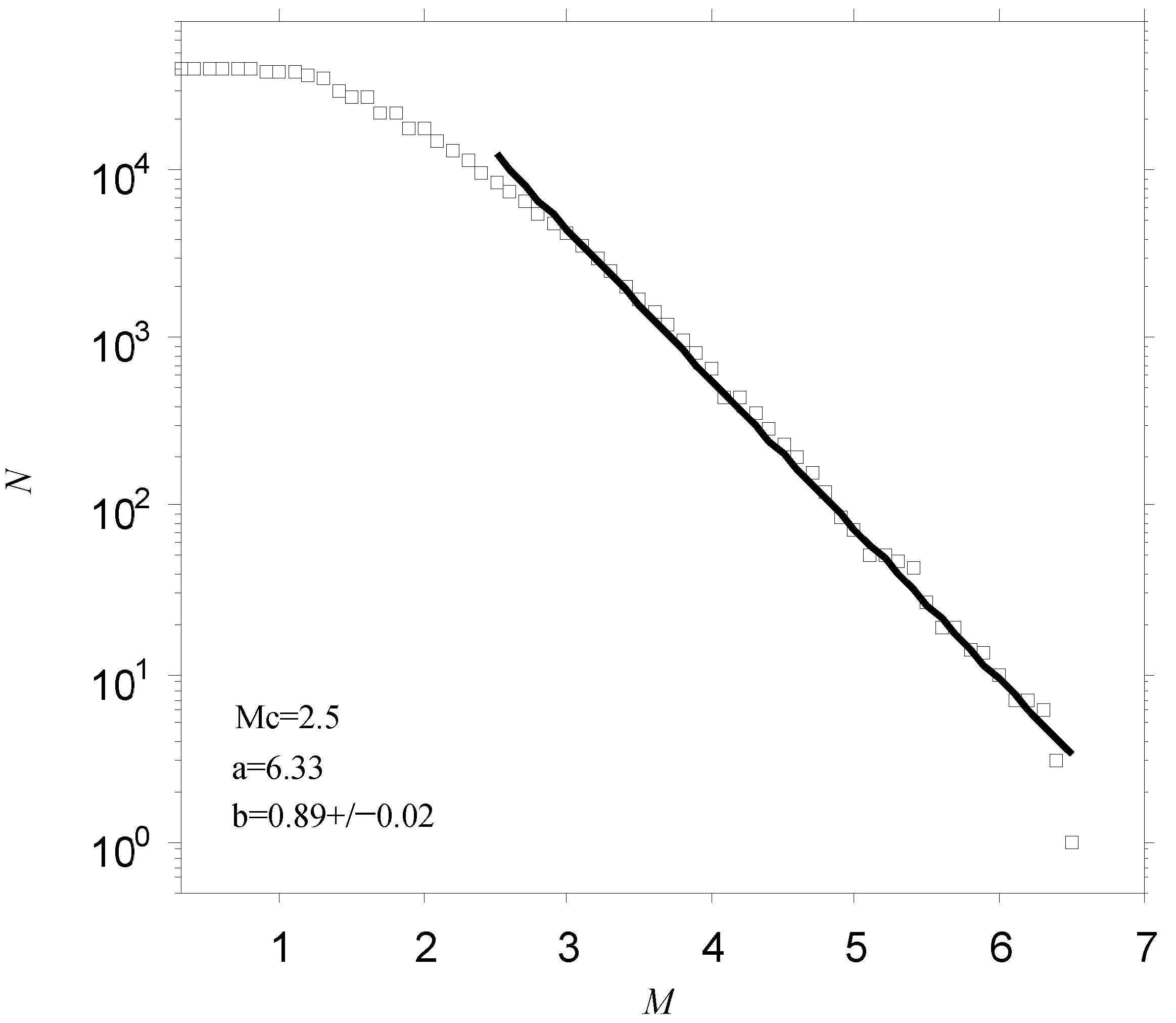
3.1. Magnitude–Frequency Relationship

The most widely used earthquake magnitude–frequency relationship is the G-R relationship [1]:

$$\log N=a+bM$$

(2)

where N is the number of earthquakes with a magnitude greater than or equal to M, the b-value characterizes the proportional relationship of the frequency of earthquakes in different magnitude intervals, and a is a parameter indicating the seismic activity rate. The most widely used method for calculating the b-value is the maximum likelihood method [10,11,12]. The procedure used for calculating the maximum likelihood method is simple but produces a large estimation error. For large samples, calculating the b-value using the least squares method is more accurate. Therefore, in this study, we used the least squares method to calculate the b-value.

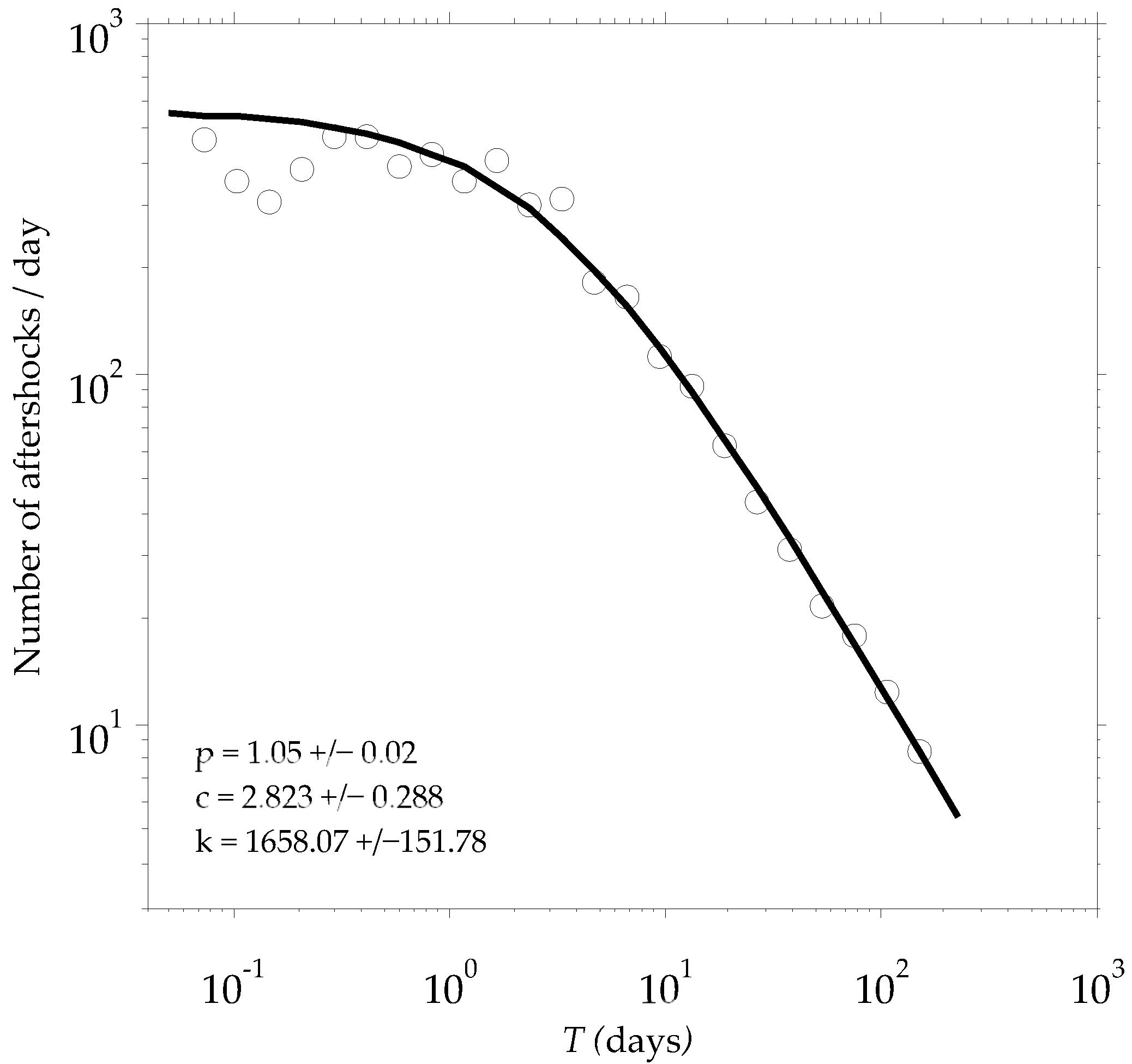
3.2. Aftershock Decay

The decay in aftershock activity over time is described by the modified Omori law [2,3]:

$$R\left(t\right)=\frac{k}{{(t+c)}^p}$$

(3)

where R(t) is the aftershock occurrence rate, and k, c, and p are constants, where p is the most important parameter that characterizes the speed of aftershock decay, and a large p-value indicates rapid aftershock decay. The p-value varies from 0.7 to 1.8 for different aftershock sequences [2], and Wiemer and Katsumata suggested that the p-value spatially varies between 0.6 and 1.4 for a single aftershock sequence [13]. The p-value is generally estimated using the nonlinear least squares method or maximum likelihood method, and we adopted the latter in this study [14].

4. Results

4.1. Statistical Characteristics of Aftershock Sequence

Figure 4 shows the relationship between the magnitude and cumulative frequency of the Wenchuan aftershock sequence. The largest aftershock of the Wenchuan earthquake was M_s 6.4 on 25 May. The least squares method was used to estimate the a- and b-values in the G-R relation and their standard deviations. According to Section 1, the data were best fit when the lower limit of the completeness magnitude M_c was 2.5, which is within the range of the variation in M_c in Figure 2. The calculations yielded a = 6.33 and b = 0.89 $\pm$ 0.02. This b-value is relatively small. The calculation of the b-value is easily affected by the magnitude interval, upper limit of the magnitude, sample size, and algorithm applied [12]. In addition, the incompleteness of the catalog is a major factor leading to errors in the b-value, and the magnitude–frequency distribution of a complete earthquake sequence is generally thought to conform to the typical G-R distribution with a b-value of one [15]. Thus, the small b-value of the Wenchuan aftershock sequence obtained in this study may be related to the absence of some small earthquakes in the catalog.

The decay of the Wenchuan aftershock activity over time is shown in Figure 5. Based on the modified Omori model [2,3], three parameters, p, c, and k, were obtained using the maximum likelihood estimation method, with M_min = M_c = 2.7 and T_start = 0.05. The calculated p-value was 1.05 $\pm$ 0.02, and the c-value was 2.823 ± 0.288. The decay pattern of the Wenchuan aftershocks conforms well to the Omori law (Figure 5), and compared with the value obtained in other studies, the p-value is normal, indicating that the background seismic activity had a minor influence on the decay of the Wenchuan aftershocks. The reason for this finding is that the magnitude and fault rupture area of the Wenchuan mainshock were both large. The seismic activities around the Wenchuan earthquake area were influenced by the ruptured fault of the mainshock over a long period.

Utsu et al. [3] showed that the p-value does not depend on the selection of M_min, while the c-value is closely related to M_min. Hence, we calculated the values of p and c for different combinations of T_start and M_min (

Table 1. Some calculations summarizing the trials for the b- and p-values for different M_min values.

No.	${\mathit{T}}_{\mathbf{start}}$ (Days)	${\mathit{M}}_{\mathbf{min}}$	p-Value	c-Value
1	0.05	2.4	1.00 ± 0.02	5.119 ± 0.485
2	0.05	2.6	1.03 ± 0.02	3.364 ± 0.335
3	0.05	2.8	1.07 ± 0.02	2.461 ± 0.259
4	0.05	3.0	1.12 ± 0.02	1.942 ± 0.218
5	0.05	3.2	1.10 ± 0.02	1.181 ± 0.156
6	0.1	2.4	1.00 ± 0.02	5.114 ± 0.491
7	0.1	2.6	1.03 ± 0.02	3.334 ± 0.339
8	0.1	2.8	1.07 ± 0.02	2.426 ± 0.263
9	0.1	3.0	1.12 ± 0.02	1.909 ± 0.222
10	0.1	3.2	1.10 ± 0.02	1.146 ± 0.160

). The p-value varied little with M_min, whereas the c-value drastically changed with M_min.

Some seismologists think that the aftershocks are so dense immediately after the mainshock that some of them overlap with each other. As a result, not all of the aftershocks can be recorded, which leads to the incompleteness of the aftershock catalog in the initial period after the mainshock, resulting in a large c-value. The c-value for a complete aftershock catalog should be zero [16]. In this study, we obtained a c-value of 2.823 ± 0.288, which is relatively large due to the incomplete aftershock catalog in the initial period after the mainshock (Figure 5). Furthermore, the complexity of the earthquake rupture process can lead to a large c-value [17]. Therefore, the large c-value in this study also suggests the complexity of the fault rupture process of the Wenchuan earthquake to a certain extent.

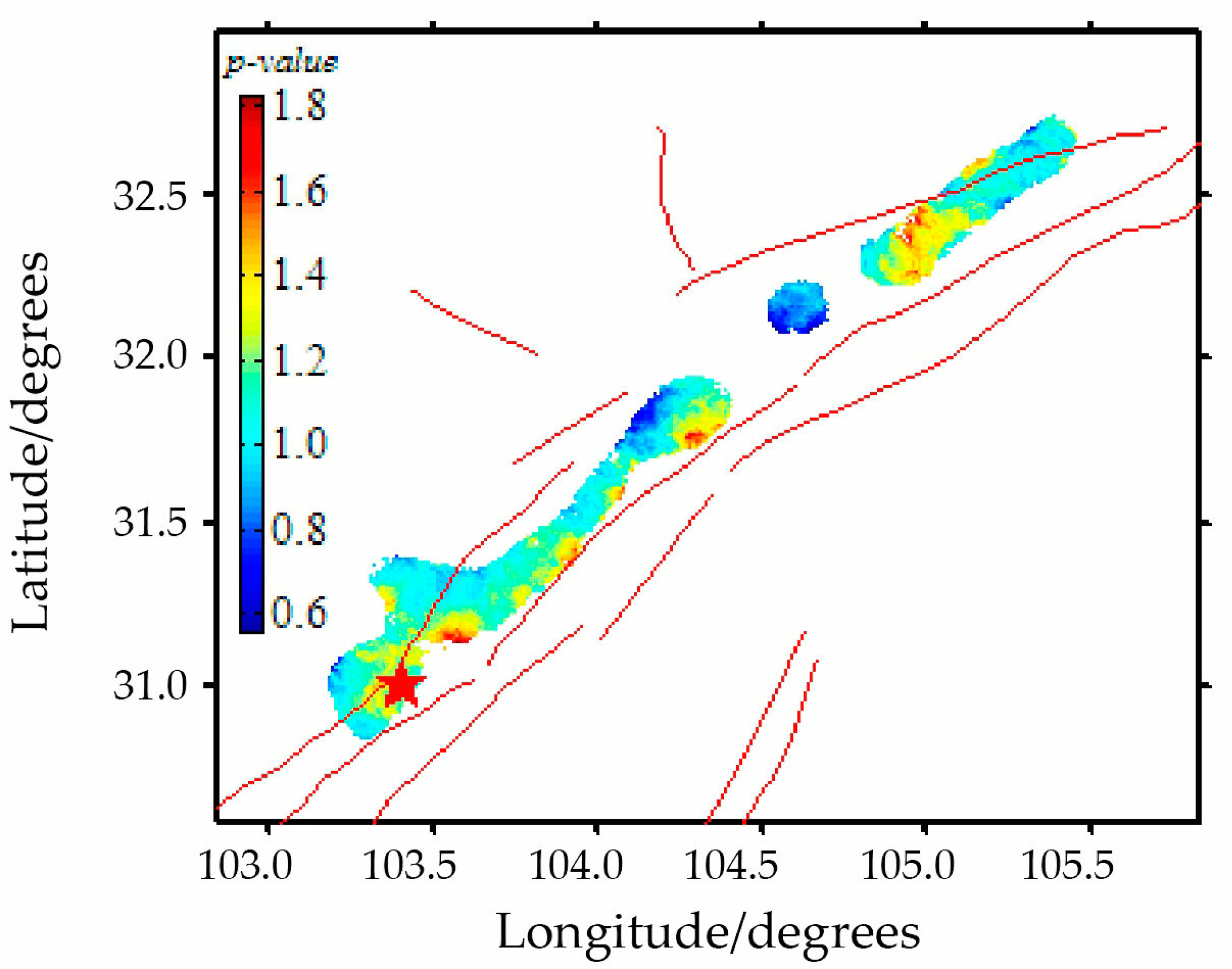
4.2. Spatial Distribution of b- and p-Values

To investigate the pattern of the spatial variation in the Wenchuan aftershock sequence, we divided the aftershock area into 0.01° × 0.01° grids and calculated the b- and p-values at each grid point (Figure 6 and Figure 7). The b- and p-values were calculated based on the earthquakes within 5 km around each grid point, and the minimum number of earthquakes required was 100, meaning the b- and p-values were calculated only when more than 100 earthquakes were within 5 km around the grid point. The calculations were performed using the ZMAP6.0 software [18].

The b-value spatially varied in the aftershock area within the range of 0.6–1.2 (Figure 6), and the b-value was generally small. The regions with relatively large b-values (b > 0.9) were mainly located around the mainshock epicenter and in the central and northeastern parts of the aftershock zone, and the area with the largest b-value was located around Qingchuan. The regions with small b-values (b ≤ 0.9) were mainly located in the southwestern part of the aftershock zone, and the area with the smallest b-value appeared at the northeast end of the aftershock zone. In addition, we found that the b-value was typically smaller along the Longmenshan central fault (i.e., near the Sichuan Basin) than along the Longmenshan back fault.

The b-value in the northeastern part of the aftershock zone was relatively large, potentially because the fault ruptures in this area were newly generated during the earthquake. The rupture mechanism was relatively simple, and the fault planes were relatively smooth, which is favorable for rapid stress adjustments. As a result, although the aftershocks were dense in this area, their intensity was low, ultimately leading to the large b-value. In the southwestern part of the aftershock zone, the aftershock intensity was relatively high because of the complex rupture mechanism, and the b-value was generally small. In addition, several strong aftershocks occurred in the southwest area of Wenchuan and at the northeast end of the aftershock zone, where the b-value was the smallest. The subsurface anomalies in these two areas may have impeded the rupture and slip of faults, leading to the occurrence of strong aftershocks and the small b-value.

The p-value spatially varied, mainly between 0.6 and 1.8 (Figure 7), which is a large range, indicating the spatial heterogeneity of the aftershock decay. A large p-value indicates the rapid decay of aftershock activity. Areas with high p-values (p ≥ 1.2) were mainly distributed in the aftershock area along the Longmenshan central fault, spreading northeast from the mainshock epicenter. The areas with the largest p-values were mainly located around Yingxiu-Hanwang, Beichuan, and Qingchuan. In contrast to the distribution pattern of large p-values, the areas with small p-values were mainly concentrated in the aftershock area along the Longmenshan back fault.

The map in Figure 7 shows that the distribution of areas with large p-values is consistent with the projection of the shallow parts of the faults on the ground. The reason for this may be that in the shallow part of the fault plane, the fault rupture mechanism was simpler than that in the deep part, the fault plane was relatively smooth, and the stress adjustments were rapid. As a result, the aftershock activity quickly decayed, and the p-value was relatively large.

5. Discussion

The spatial distributions of b- and p-values of the aftershock sequence provide useful information for interpreting the rupture mechanisms of earthquakes and understanding the properties of the media in the earthquake area. The spatial variations in these two values may be related to tectonic conditions, rock anisotropy, stress states, surface heat flow, and fault slip in the earthquake area, but no evidence exists to show which factor is the main cause of their variations [19]. Eaton et al. [20] investigated the characteristics of the spatial distribution of b- and p-values for the aftershock sequence of the Parkfield earthquake. Since then, many studies have been conducted on the spatial distribution of b- and p-values, some of which have shown that the spatial variation in the aftershock b-value is related to stress: a low b-value after the mainshock indicates that the earthquake area was subjected to high stress [5,21,22,23]. Kisslinger and Jones [2] studied the temporal characteristics of the aftershock sequences of 39 earthquakes in California, USA and did not find a correlation between the p-value and the b-value of the aftershock sequences or the magnitude of the mainshock. However, they observed that the p-value varied from 0.688 to 1.809 and concluded that the p-value is related to the surface heat flow. Guo and Ogata [24] focused on the aftershock sequences of 34 earthquakes in Japan during the 1971–1995 period and concluded that the aftershock parameters of inland earthquakes are mainly affected by the surface heat flow or the anisotropy of the rock structure in the earthquake area. Thereafter, Wiemer and Katsumata [13] simultaneously analyzed the spatial variations in the b- and p-values for four aftershock sequences of the Kobe, Morgan Hill, Landers, and Northridge earthquakes, and their findings complement the results obtained by Kisslinger and Jones [2] and Guo and Ogata [24]. They concluded that although the magnitude–frequency distribution is controlled by shear stress, crack density, and pore pressure, the b-value is correlated with the amount of fault slip in the mainshock rupture zone, and the b-value tends to be high in areas with maximum fault slip. Enescu and Ito [23] investigated the spatial distributions of b- and p-values for the aftershock sequence of the 2000 Western Tottori earthquake. They found that the b-value was associated with the stress distribution pattern in the earthquake area after the mainshock, whereas the p-value was related to the amount of fault slip in the mainshock rupture zone, and a large p-value corresponded to a large amount of fault slip.

Zhang et al. [25] studied the spatiotemporal rupture process of the Wenchuan earthquake and discovered four areas with concentrated fault slip on the earthquake rupture plane. The largest fault slips were beneath the Wenchuan-Yingxiu area, with a maximum fault slip of 7.3 m, and near the Beichuan area, with a fault slip of 5.6 m. In addition, fault slips were concentrated in the areas of Qingchuan and Kangding, but their scales were smaller than those in the above two areas. Subsequently, Wang et al. [26] analyzed the source process of the Wenchuan earthquake and provided the spatial distribution of fault slip during the mainshock. Their results are consistent with those of Zhang et al. [25], but the values differ. We compared the spatial distribution of the calculated b-value with the abovementioned fault slip distribution and did not find consistency between the two. According to Wiemer and Katsumata [13], the b-value should be large in the region with the largest amount of fault slip, which does not align with our findings. Then, we compared the spatial distribution of the calculated p-value (Figure 7) with the fault slip distribution and found that the two are correlated. The spatial distribution of areas with large p-values is consistent with the fault slip distribution pattern obtained by Wang et al. [26], especially in Yingxiu-Hanwang, Beichuan, and Qingchuan, which are areas with a concentrated fault slip, and the p-value linearly correlated with the amount of fault slip. In addition, we found that the b- and p-values were both large in the Qingchuan area, and Bayrak and Öztürk [14] suggested that special geotectonic conditions (e.g., the Holocene alluvial sedimentary structure) may lead to increases in the b- and p-values. Therefore, we inferred that special geotectonic structures may be present in the vicinity of Qingchuan.

Parsons et al. [27] calculated the changes in the stress in the earthquake area after the Wenchuan mainshock, finding that the stress increased at the intersection of the Longmenshan fault and the Sichuan Basin. Coulomb stress substantially increased in the south of the mainshock fault, and the stress in the Qingchuan and Huya areas decreased. This pattern shows a correlation with the spatial distribution of the b-value that we calculated. As described in Section 3, the b-value was generally small in the earthquake area along the Longmenshan front fault (i.e., the area intersecting the Sichuan Basin) and the southwestern part of the aftershock area, and the b-value was the largest in the Qingchuan area, indicating that areas with large and small b-values may correspond to the regions experiencing small and large stresses, respectively. However, no information is available on the decreases or increases in stress in the areas around the mainshock epicenter, where the b-value was large, and at the northeast end of the aftershock area, where the b-value was the smallest. Based on the above results, we speculate that the stress decreased and increased in these areas, respectively. Moreover, these two areas are located near the starting and end points of the mainshock rupture, so we speculate that subsurface anomalies may exist in these two areas.

Ogata et al. [28] found that the variations in b-values agree with friction-related seismic velocity perturbations and stated that the regions with high and low b-values correspond to relatively low and high P-wave velocities, respectively. In addition, Young and Maxwell [29] also demonstrated that a region with high seismic wave velocity may be a region that is subjected to high stress. Wu et al. [30] studied the three-dimensional P-wave velocity structure in and around the Wenchuan earthquake area. Their results showed widespread high-velocity anomalies at a depth within 20 km of the surface in the crust along the Longmenshan fault, which is consistent with the typically small b-values in the aftershock zone revealed in our study. By comparing the spatial distribution of the b-value calculated in this study with the distribution of three-dimensional P-wave velocity anomalies reported by Wu et al. [30], we found that low P-wave velocity anomalies appeared in areas with large b-values, with high-velocity anomalies being found in the areas with small b-values, especially at the northeast end of the aftershock zone, where the high-velocity anomalies along the Ningqiang-Mianxian region [30] may have been responsible for the small b-values. In addition, we compared the spatial distribution of the b-value with the apparent velocity structure in the Longmenshan fault zone and its surroundings calculated by Lou et al. [31]. We found that the apparent velocities were relatively high in the areas with small b-values and relatively low in the areas with large b-values. The above findings show that the spatial distribution of the b-value in the aftershock region is closely related to the properties of the media in the earthquake area.

6. Conclusions

In this study, we thoroughly investigated the Wenchuan aftershock activity, and our conclusions are as follows:

According to the G-R equation [1], M_c was found to have a magnitude of 2.5, and the b-value of the Wenchuan aftershock sequence was calculated to be 0.89 ± 0.02, which is relatively small. The small b-value may have been caused by the absence of small earthquakes in the catalog. In addition, the physical properties of the media in the earthquake area are factors that could have led to the small b-value.

According to the modified Omori law [2,3], the pattern of decay in the Wenchuan aftershocks was studied, and the p- and c-values obtained were 1.05 ± 0.02 and 3.00, respectively. We found that the Wenchuan aftershock sequence conforms well to the Omori formula. The p-value varied little with M_min, whereas the c-value drastically varied with the change in M_min. The absence of the aftershock records in the first few hours after the mainshock and the complexity of the source rupture process were responsible for the large c-value.

The b-value spatially varied from 0.6 to 1.2 in the aftershock zone (Figure 6) and was generally small. The areas with relatively large b-values (b > 0.9) were mainly located near the mainshock epicenter and in the central and northeastern parts of the aftershock zone. The areas with relatively small b-values (b ≤ 0.9) were located in the southwestern part of the aftershock zone. The relatively large b-values in the northeastern part of the aftershock zone may have been caused by the fault ruptures in this area that were newly generated during the earthquake. The rupture mechanism was relatively simple, and the fault planes were relatively smooth, which was favorable for rapid stress adjustments. As a result, although the aftershocks were dense in this area, their intensity was low, ultimately leading to the large b-value. In the southwestern part of the aftershock zone, the aftershock intensity was relatively high because of the complex rupture mechanism, and the b-value was generally small. In addition, several strong aftershocks occurred in the southwest area of Wenchuan and at the northeast end of the aftershock zone, where the b-value was the smallest. The subsurface anomalies in these two areas may have impeded the rupture and slip of faults, leading to the occurrence of strong aftershocks and the small b-value.

The p-value spatially varied mainly between 0.6 and 1.8 (Figure 7), which is a large variation range, indicating the spatial heterogeneity of the aftershock decay. A large p-value indicates the rapid decay of aftershock activity. The areas with high p-values (p ≥ 1.2) were mainly distributed in the aftershock area along the Longmenshan central fault, spreading northeast from the mainshock epicenter. Moreover, the distribution of areas with large p-values is consistent with the projection of shallow parts of the faults on the ground. The reason for this may be that in the shallow part of the fault plane, the fault rupture mechanism was simpler than that in the deep part, the fault plane was relatively smooth, and the stress adjustments were rapid. As a result, the aftershock activity quickly decayed, and the p-value was relatively large.

The spatial variations in the b- and p-values were related to the earthquake source mechanism and the physical properties of the rock media. We compared the spatial distribution of the calculated b-values (Figure 6) and p-values (Figure 7) with other results for the Wenchuan earthquake [25,26,27,30,31] and found that the spatial variation in the b-value may have been related to the P-wave velocity, density of the media, and the stress change in the earthquake area. The spatial variation in the p-value was closely related to the amount of fault slip during the mainshock, and the two showed a strong linear correlation. Therefore, we think that the spatial variation in the b-value may have been predominantly controlled by the petrophysical properties of the crust in the earthquake area. The spatial variation in the p-value may have been more closely related to the earthquake focal mechanism.

With the application of artificial intelligence technology in earthquake phase picking, lower-magnitude earthquakes can be obtained, and more statistical samples can be obtained. This will allow us to obtain more precise statistical results, making it easier for us to objectively and scientifically understand the process of earthquake preparation and rupture.

References

1. Gutenberg, R.; Richter, C.F. Frequency of earthquakes in California. Bull. Seism. Soc. Am. 1944, 34, 185–188. [Google Scholar] [CrossRef]
2. Kisslinger, C.; Jones, L.M. Properties of aftershocks in southern California. J. Geophys. Res. 1991, 96, 11947–11958. [Google Scholar] [CrossRef]
3. Utsu, T.; Ogata, Y.; Matsu’ura, R.S. The centenary of the Omori formula for a decay law of aftershock activity. J. Phys. Earth 1995, 43, 1–33. [Google Scholar] [CrossRef]
4. Wiemer, S.; Wyss, M. Minimum magnitude of completeness in earthquake catalogs: Examples from Alaska, the western US and Japan. Bull. Seism. Soc. Am. 2000, 90, 859–869. [Google Scholar] [CrossRef]
5. Tropeano, G.; Simoncelli, M. On the influence of Shallow Underground Structures in the Evaluation of seismic signals. Ing. Sismica 2021, 38, 23–35. [Google Scholar]
6. Jia, K.; Zhou, S.; Zhuang, J.; Jiang, C. Possibility of the independence between the 2013 Lushan earthquake and the 2008 Wenchuan earthquake on Longmen Shan Fault, Sichuan, China. Seism. Res. Lett. 2014, 85, 60–67. [Google Scholar] [CrossRef]
7. Jia, K.; Zhou, S.; Zhuang, J.; Jiang, C. Stress transfer along the western boundary of the Bayan Har Block on the Tibet Plateau from the 2008 to 2020 Yutian earthquake sequence in China. Geophys. Res. Lett. 2021, 48, e2021GL094125. [Google Scholar] [CrossRef]
8. Jiang, C.S.; Wu, Z.L.; Zhuang, J.C. ETAS model applied to the earthquake-sequence association (ESA) problem: The Tangshan sequence. Chin. J. Geophys. 2013, 56, 2971–2981. (In Chinese) [Google Scholar]
9. Wiemer, S.; McNutt, S.R.; Wyss, M. Temporal and three dimensional spatial analysis of the frequency-magnitude distribution near Long Valley Caldera, California. Geophys. J. Int. 1998, 134, 409–421. [Google Scholar] [CrossRef]
10. Aki, K. Maximum likelihood estimate of b in the formula log N = abM and its confidence limits. Bull. Earthq. Res. Inst. Univ. Tokyo 1965, 43, 237–239. [Google Scholar]
11. Shi, Y.; Bolt, B.A. The standard error of the magnitude–frequency b value. Bull. Seism. Soc. Am. 1982, 72, 1677–1687. [Google Scholar] [CrossRef]
12. Bender, B. Maximum likelihood estimation of b-values for magnitude grouped data. Bull. Seism. Soc. Am. 1983, 73, 831–851. [Google Scholar] [CrossRef]
13. Wiemer, S.; Katsumata, K. Spatial variability of seismicity parameters in aftershock zones. J. Geophys. Res. 1999, 104, 13135–13151. [Google Scholar] [CrossRef]
14. Ogata, Y. Estimation of the parameters in the modified Omori formula for aftershock frequencies by the Maximum Likelihood procedure. J. Phys. Earth 1983, 31, 115–124. [Google Scholar] [CrossRef]
15. Bayrak, Y.; Öztürk, S. Spatial and temporal variations of the aftershock sequences of the 1999 İzmit and Düzce earthquakes. Earth Planets Space 2004, 56, 933–944. [Google Scholar] [CrossRef]
16. Utsu, T. Aftershock and earthquake statistic (III): Analyses of the distribution of earthquakes in magnitude, time and space with special consideration to clustering characteristics of earthquake occurrence (1). J. Fac. Sci. Hokkaido Univ. Ser. VII (Geophys.) 1971, 3, 379–441. [Google Scholar]
17. Yamakawa, N. Foreshocks, aftershocks, and earthquake swarms (IV)—Frequency decrease of aftershocks in its initial and later stages. Pap. Met. Geophys. 1968, 19, 109–119. [Google Scholar] [CrossRef]
18. Wiemer, S. A Software Package to Analyze Seismicity: ZMAP. Seismol. Res. Lett. 2001, 72, 374–383. [Google Scholar] [CrossRef]
19. Öztürk, S.; Çinar, H.; Bayrak, Y.; Karsli, H.; Daniel, G. Properties of the Aftershock Sequences of the 2003 Bingöl, MD = 6.4, (Turkey) Earthquake. Pure Appl. Geophys. 2008, 165, 349–371. [Google Scholar] [CrossRef]
20. Eaton, J.; O’Neil, M.; Murdock, J. Aftershocks of the 1966 Parkfield- Cholame, California, earthquake: A detailed study. Bull. Seismol. Soc. Am. 1970, 60, 1151–1197. [Google Scholar]
21. Frohlich, C.; Davis, S. Teleseismic b-values: Or, much ado about 1.0. J. Geophys. Res. 1993, 98, 631–644. [Google Scholar] [CrossRef]
22. Wiemer, S.; Wyss, M. Mapping the frequency-magnitude distribution in asperities: An improved technique to calculate recurrence times. J. Geophys. Res. 1997, 102, 15115–15128. [Google Scholar]
23. Enescu, B.; Ito, K. Spatial analysis of the frequency-magnitude distribution and decay rate of aftershock activity of the 2000 Western Tottori earthquake. Earth Planets Space 2002, 54, 847–859. [Google Scholar] [CrossRef]
24. Guo, Z.; Ogata, Y. Statistical relation between the parameters of aftershocks in time, space, and magnitude. J. Geophys. Res. 1997, 102, 2857–2873. [Google Scholar] [CrossRef]
25. Zhang, Y.; Feng, W.P.; Xu, L.S.; Zhou, C.H.; Chen, Y.T. Space time rupture process of 2008Wenchuan earthquake. Sci. China 2008, 38, 1186–1194. (In Chinese) [Google Scholar]
26. Wang, W.M.; Zhao, L.Z.; Li, J.; Kang, Y. Rupture process of the M 8.0 Wenchuan earthquake of Sichuan, China. Chin. J. Geophys. 2008, 51, 1403–1410. (In Chinese) [Google Scholar]
27. Parsons, T.; Ji, C.; Kirby, E. Stress changes from the 2008 Wenchuan earthquake and increased hazard in the Sichuan basin. Nature 2008, 454, 509–510. [Google Scholar] [CrossRef] [PubMed]
28. Ogata, Y.; Imoto, M.; Katsura, K. 3-D spatial variation of b-values of magnitude-frequency distribution beneath the Kanto District, Japan. Geophys. J. Int. 1991, 104, 138–146. [Google Scholar] [CrossRef]
29. Young, R.P.; Maxwell, S.C. Seismic characterization of a highly stressed rock mass using tomographic imaging and induced seismicity. Geophys. Res. 1992, 97, 12361–12373. [Google Scholar] [CrossRef]
30. Wu, J.P.; Huang, Y.; Zhang, T.Z.; Ming, Y.H.; Fang, L.H. Aftershock distribution of the Ms 8.0 Wenchuan earthquake and three dimensional P-wave velocity structure in and around source region. Chin. J. Geophys. 2009, 52, 320–328. (In Chinese) [Google Scholar]
31. Lou, H.; Wang, C.Y.; Lü, Z.Y. Deep structural environment of 2008 Wenchuan Ms 8.0 earthquake: Joint interpretation from teleseismic P-wave receiver function and Bouger gravity anomaly. Sci. China 2008, 38, 1207–1220. (In Chinese) [Google Scholar]
Figure 1. A map of the Wenchuan aftershock sequence. The circles mark the aftershocks, and the symbol size is proportional to the magnitude. The red star marks the mainshock hypocenter location. F1, Longmenshan back fault; F2, Longmenshan central fault; F3, Longmenshan front fault.
Applsci 14 04754 g001
Figure 2. The magnitude of completeness, Mc, as a function of time for the Wenchuan aftershock sequence.
Applsci 14 04754 g002
Figure 3. A surface map of the spatial distribution of Mc for the Wenchuan aftershock sequence. The red star marks the hypocenter location of the mainshock.
Applsci 14 04754 g003
Figure 4. Frequency–magnitude distributions of Wenchuan aftershock sequence.
Applsci 14 04754 g004
Figure 5. Decay rate of aftershock activity over time after mainshock.
Applsci 14 04754 g005
Figure 6. Spatial distribution of b-value for Wenchuan aftershock sequence. Red star marks mainshock hypocenter location; red lines mark faults.
Applsci 14 04754 g006
Figure 7. Spatial distribution of Wenchuan aftershock sequence. Red star marks mainshock hypocenter location; red lines mark faults.
Applsci 14 04754 g007