Abstract
Time-domain numerical simulation is generally considered an accurate method to predict the mooring system performance, but it is also time and resource-consuming. This paper attempts to completely replace the time-domain numerical simulation with machine learning approaches, using a catenary anchor leg mooring (CALM) system design as an example. An adaptive sampling method is proposed to determine the dataset of various parameters in the CALM mooring system in order to train and validate the generated machine learning models. Reasonable prediction accuracy is achieved by the five assessed machine learning algorithms, namely random forest, extremely randomized trees, K-nearest neighbor, decision tree, and gradient boosting decision tree, among which random forest is found to perform the best if the sampling density is high enough.
1. Introduction
A mooring system is usually used for an offshore floating structure to maintain its upright position, which is a traditional approach compared to the dynamic positioner. However, mooring system incidents have occurred at an increasing rate [1]. To ensure the operational safety of the mooring system, a lot of research focusing on its design and failure detection, using machine learning methods, has been conducted in recent years.
The design of the mooring system has been hindered by the low efficiency of time-domain numerical calculation for a long time. Compared with the static or frequency-domain method, time-domain numerical simulation is regarded as the more accurate method for mooring analysis despite being more computationally demanding. With the advancement of computing technology, time-domain numerical simulation has become feasible in mooring design.
Nevertheless, efficiency is still a significant limitation when it comes to the optimization design, which requires a lot of calculation cases as the basis data. As a result, static mooring analysis has been adopted and combined with the genetic algorithm to perform mooring optimization design [2].
Later, the machine learning method was introduced to make quick and accurate predictions, replacing the time-domain simulation and lifting the efficiency limitation on optimization problems. For a floating offshore platform anchored by 18 mooring lines distributed in four clusters, a hybrid method combining finite element analysis and artificial neural networks (ANN) for fatigue analysis has been proposed, to balance the accuracy and efficiency of simulating multiple sea states [3]. They also used ANN to reduce computational efforts in truncated model tests [4,5] performed a floating wind turbine (FOWTs) aero-hydro-servo-elastic modeling to assess the effects of mooring line tension via deep learning, and the major contributing factors were identified by ANN [6,7] assessed mooring system design optimization using the multi-objective genetic algorithm assisted by a random forest-based surrogate model. Recently, a new artificial intelligence-based method named SADA was proposed for the prediction of dynamic responses [8]. For a 4 point tanker–buoy mooring system, the simulation results of mooring tensions and tanker motion displacements by Ocraflex have been employed to train ANN structure, and an algorithm was created to obtain quick predictions [9,10], which achieved time-domain simulation by a BP neural network using the calculation results from Moses as training samples for pipe-laying vessels. Pipe movement was significantly reduced at different wave direction angles using the genetic optimization algorithm. For a vessel-shaped offshore fishing farm, ref. [11] applied the Kriging metamodels as surrogates for calculating the time-domain responses. The optimal solutions were found by exploring the design space using a gradient-based search algorithm.
During the mooring system building process, structural health monitoring could be achieved by machine learning methods to make real-time predictions based on previous field data or numerical simulation results [12,13]. For a semisubmersible with mooring lines, an ANN model was used for the prediction of mooring line tensions and fatigue assessment [14]. The model was trained using time histories of vessel motions and the corresponding mooring line tensions for a range of sea states generated by numerical simulations. The monitored motion of the platform is used to predict the mooring line damage based on the results of the ANN model trained using the results from numerical analyses. This method was also adapted for spread-moored FSPO [15]. For the spread-moored FSPO, neural networks trained by measured motion were also used to detect mooring line failure in near real-time [16,17]. Saad et al., 2021; Sidarta et al., 2019, on the other hand, trained the neural networks using FPSO response to a range of Metocean conditions by numerical simulations. For turret-moored FSPO, Metocean and GPS data from an FPSO were used to train Kriging and neural network models, and the identified mooring system change was used to predict a mooring line failure event [18]. For the tension leg platform (TLP), ref. [19] used deep neural networks (DNN) to detect mooring line damage based on simulation data using Charm3D (a fully coupled nonlinear hull/mooring/riser program from Texas A&M University, College Station, TX, USA). DNN was also used to detect mooring line failure based on the data from floater–mooring coupled hydroelastic time-domain numerical simulations for the submerged floating tunnel (SFT) [20].
Until now, time-domain numerical simulation has been a common practice in both mooring system design and detection. To replace this time-consuming approach, the most recent research focused on the neural networks, and only a few assessed other methods, such as Kriging and random forest.
This paper investigates five popular machine learning algorithms, including random forest, extremely randomized trees, K-nearest neighbor, decision tree, and gradient boosting decision tree, to substitute time-domain mooring numerical simulation, using the CALM case as an example. In addition, a sampling strategy for global and local data is proposed to select the numerical basis cases.
2. Data from Numerical Simulation of the CALM System
2.1. Numerical Simulation in CALM Design
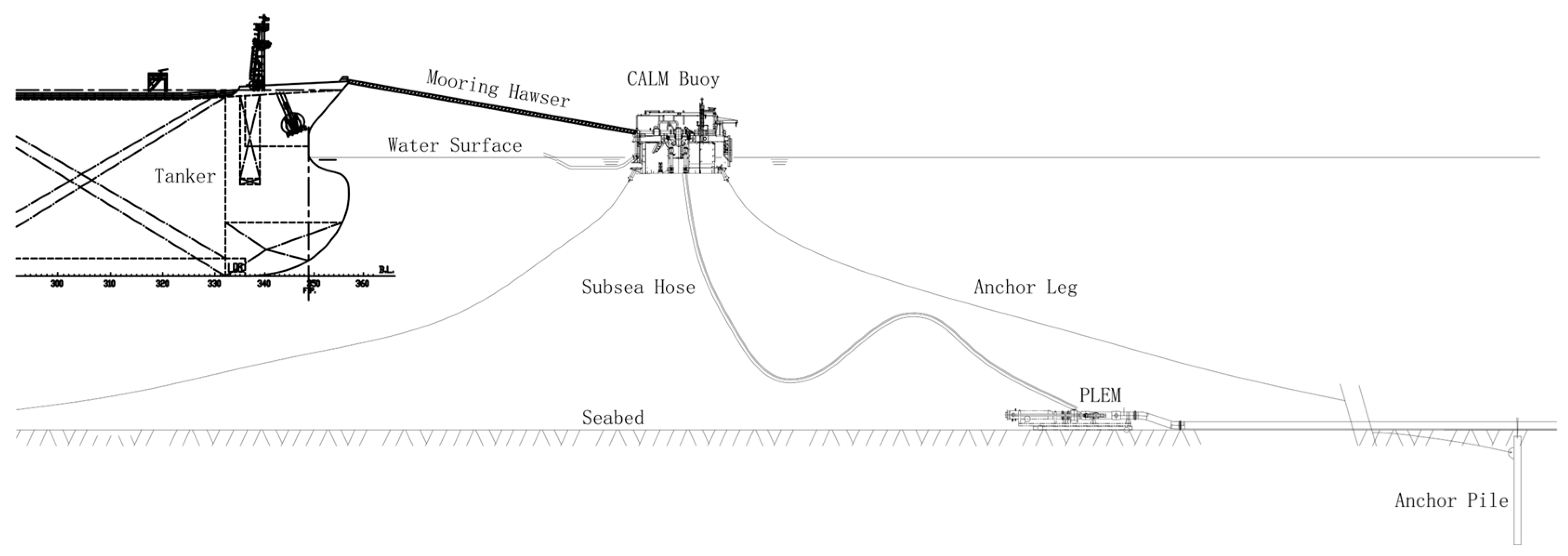
The CALM (Catenary Anchor Leg Mooring) system, deployed in shallow water, usually consists of a floating buoy, six anchoring lines, and a pair of mooring hawsers, as shown in Figure 1. For a normal field environment, the design conditions can be divided into two groups:

Figure 1.
Schematic of the CALM system.
- (1)
- Operation condition: A tanker with full loading and ballast loading is connected to the CALM buoy by mooring hawsers.
- (2)
- Self condition: CALM buoy stands alone without the tanker connected.
In each condition, the environmental loads need to be divided into several groups. Despite the actual complex conditions, a simplified method is adopted to deal with the environmental loads. For normal environmental conditions, wind, current, and wave in collinear and non-collinear directions are considered. “Collinear” refers to the situation where wind, current, and wave are in the same direction, whereas “non-collinear” implies that wind and current have a 30 and 45 degree deviation from the wave, respectively. The direction of the resultant load can either be aligned with one of the anchor legs or between two legs. According to DNV and ABS regulations [21,22], one mooring line failure situation is analyzed for each governing case in addition to the intact analysis with no mooring line failure. The mooring line numbering scheme is defined in Figure 2. As a result of the symmetrical configuration, mooring line 1 or 2 is assumed to be the failure line. There are, therefore, 10 cases to be assessed if different failing mooring lines and load directions are considered, as shown in Figure 2. Since two operation conditions (full loading and ballast loading) and the self condition need to be investigated, 30 cases need to be simulated for a design assessment. The other design parameters, namely CALM buoy and VLCC (Very Large Crude Carrier), are fixed to simplify the problem.
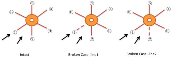
Figure 2.
Mooring line numbering scheme and definition of environmental loads’ heading direction (resultant load).
In order to verify the feasibility of the mooring design, it is necessary to evaluate the results of buoy offset, anchor line laid length, anchor line tension, and hawser tension from the numerical simulation. According to the ABS regulation [21], the minimum factor of safety against the breakage of each anchor leg component is used, while the DNV regulation [22] employs a utilization factor.
The input and output parameters of the operation and self condition modules are presented in Figure 3 and summarized as follows. vw means wind speed, vc means flow velocity, hs means wave height, tp means wave spectrum period, moor_d means water depth, d means anchor chain’s diameter, pta means pretension angle, cable_L means length of cable, cable_stiff_p means cable stiff primary coefficient, cable_stiff_q means cable stiff quadratic coefficient, cable_br means cable strength, CN means working condition, minlaidl means minimum left length of cable, max_hawserC means maximal cable force utility factor, maxchainFC means maximum chain force factor, maxchainFC_DNV means maximum chain force factor according to DNV, maxoffsetC means maximum offset of the buoy. Case No. is an integer value starting from 0 to 9, totaling 10 cases as mentioned above.
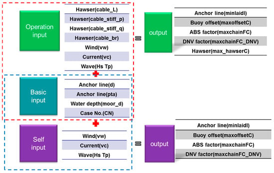
Figure 3.
Input and output parameters of AQWA.
The numerical simulation in the paper is performed by ANSYS AQWA software (version 11.0). The output parameters obtained through simulation and the input parameters form the dataset for training the machine learning models. To accelerate the calculation, a special program is built on the cloud platform to realize parallel computing.
2.2. Sampling Strategy
The simulation base dataset should be obtained using an appropriate sampling method to ensure high machine learning accuracy, which depends on the sampling approach, sampling amplitude, and sampling density. In this work, Latin Hypercube sampling, a form of stratified sampling method with approximately random sampling seed across the distribution of multiple parameters [23,24], is adopted given the multiple dimensions of the input data. Due to the demanding resource consumption of numerical simulation, it is unrealistic to sample the data globally as much as possible to achieve satisfactory accuracy. The overall data can be mainly divided into global and local data. If the prediction made by the model trained by global data is poor, local data should be tested, in which case a resultant high accuracy means that the local data density could be applied in the global data range.
The data range, test data value, and the minimum sampling accuracy for the self and operation conditions are shown in Table 1 and Table 2, respectively. All the data are sampled within the specified range, and local data are sampled with a certain deviation around the test value. The local data are sampled by two-precision and three-precision rules. The former samples two values for each input dimension around the test value by a difference equal to the sampling accuracy. For example, the vw values sampled for the operation condition are 21.9 and 22.1, according to the two-precision rule. Similarly, the three-precision rule samples three values around the test value, including the test value itself (21.9, 22, and 22.1 for the aforementioned example). In order to guarantee the validity of the training dataset, the value combinations which are the same as the test dataset are eliminated.

Table 1.
Data sampling information for the operation condition (d is a discrete value which can only be sampled according to the manufacturer’s table, and cabel_br is constant to simplify the parameter values).

Table 2.
Data sampling information for the self condition (d is a discrete value which can only be sampled according to the manufacturer’s table).
More refined structures for global data and local data are shown in Figure 4 and Figure 5. Because operation calculation is more complicated and time-consuming, the size of the operation condition dataset is made smaller than the self condition dataset to achieve a similar level of computation time. Three datasets are sampled in the operation condition, as illustrated in Figure 4. Dataset 1 (global_1) includes 81 data in the global area sampled by Latin hypercube, which makes the total number of cases 1620, considering 20 working conditions for each sampled global data. Dataset 2 adds 337 global data and two-precision sampled local data to dataset 1. The total amount of added data is 10,240, composed of 6740 (337 20) global data and 5120 local data, which are the combination of the two-precision data of eight input parameters (28) and working conditions (28 20). Dataset 3 adds 131,220 (38 20) three-precision method sampled data to the dataset. However, the model was later shown to achieve satisfactory performance with fewer data, so 49,020 data were used.
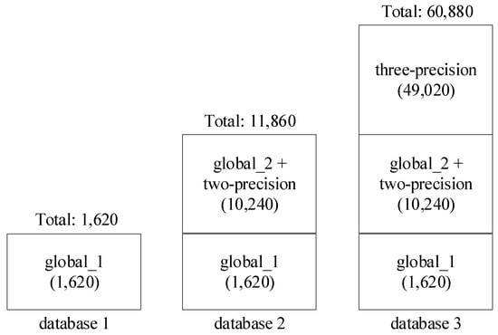
Figure 4.
Sampling structure for operation’s datasets.
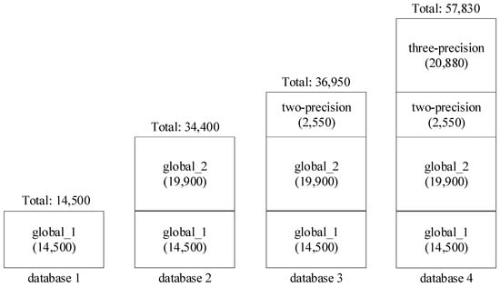
Figure 5.
Sampling structure for self condition datasets.
Four datasets are sampled for the self condition, as shown in Figure 5. Dataset 1 (global_1) constitutes 1450 data in the global area by the Latin hypercube sampling method, making the total data 14,500 given 10 working conditions. Dataset 2 adds 19,900 (1990 10) global data to dataset 1. Dataset 3 takes two-precision sampling to include 1280 (27 × 10) local data (the exponent 7 refers to 7 input parameters). Some experiments are performed to refine the sampling accuracy, and 1270 local data are added, making the total local data 2550. Dataset 4 further includes 21,870 (37 × 10) local data by three-precision sampling. With the repetitive data by two-precision sampling excluded, 20,880 data are added in addition to Dataset 3.
For evaluating the accuracy of the machine learning model, the dataset is further divided into three parts: training dataset, validation dataset, and test dataset, as shown in Figure 6. The training dataset is used to train the models, and the validation dataset and test dataset are both used to assess the prediction accuracy of the trained model. The main difference between the validation and test dataset is that the former is sampled by the same approach as the training dataset, whereas the latter is collected from the actual engineering data. Therefore, the accuracy of the model assessed by the test dataset is typically lower than the validation dataset. In this work, 80% of the total sampled data are designated as the training dataset, and the rest forms the validation dataset, which is a practice called 5-fold cross validation.
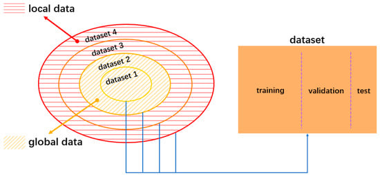
Figure 6.
Machine learning data structure.
3. Machine Learning Method
This section introduces the machine learning models to be accessed in the following sections and describes the method to quantify their corresponding prediction accuracy.
3.1. Machine Learning Models
3.1.1. Decision Tree (DT)
The decision tree continuously divides the dataset through judgment conditions and finally obtains the classification or regression model of the tree [25]. This research employs a regression decision tree. To facilitate understanding, the regression decision tree generated by the first five self condition training data is presented as an example in Figure 7.
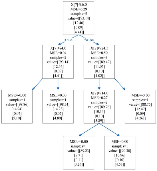
Figure 7.
Flow chart of the regression decision tree.
X represents the multiple features (i.e., working conditions) of the input data. Samples refer to the number of samples contained in the node, and the value represents the average value of the samples contained in the node in different output dimensions. denotes mean squared error and can be expressed as:
where m means the number of samples contained in the node, and represent the model input and output (i.e., prediction), and is the actual value. The regression decision tree selects a certain value of the input feature as the division point and divides the left subtree and the right subtree according to the comparison of the division point’s value. The criterion for selecting the division point is that the predicted value after division is closer to the true value. In this case, is used as the criterion for dividing points. In each division, after the are calculated with all input features used as the dividing points, the one with the most decrease in mse is selected as the dividing point. The decision tree is fully constructed when each leaf node contains only one sample. When predictions are made, the input data continuously enter the branch according to the judgment condition of each node and finally reaches the leaf node. The average of the leaf node value in each dimension is taken as the predicted value.
3.1.2. Random Forest (RF)
Random forest is an extended variant of Bagging, which belongs to the ensemble learning method [26,27,28]. The idea is that, given a dataset containing m samples, the sample may still be selected in the next sampling so that the dataset still contains m samples after m random sampling operations. Some samples of the initial training dataset appear multiple times in the sampling set, while the others never appear again. About 63.2% of the samples in the initial training dataset are included in the sampling set, as suggested by Equation (2).
According to this approach, there can be T sample sets containing m training samples. Then, a base learner is trained based on each sample set before the trained base learners are combined. Random forest is evolved from the construction of the Bagging integration of decision tree learners, and further introduces random attribute selection in the training process of decision trees. The decision tree selects an optimal attribute from the attribute set of the current node when selecting the partition attribute. For each node in the random forest, a subset with k attributes is first randomly selected from the attribute set of the node before an optimal attribute of the subset is picked for division. The diversity of base learners in the random forest owes to sample disturbances and attribute disturbances. As a result, the generalization performance of the final integration can be further improved by increasing the difference between individual learners.
3.1.3. Extremely Randomized Trees (ET)
Extremely randomized trees [29] are modified based on the random forest to enhance the randomness. Both extremely randomized trees and random forest build the Bagging ensemble based on the decision tree and introduce random attribute selection in the training of the decision tree. The difference is that extremely randomized trees also use random methods when selecting division points for random attributes. The decision tree relies on information gain or improved purity to select the division point of attributes, whereas extremely randomized trees randomly select values in the attribute interval as the division point. Compared with random forest, extremely randomized trees reduce variance while increasing bias. The problem of large deviation can be solved by appropriately adjusting the randomization level.
3.1.4. Gradient Boosting Decision Tree (GBDT)
The boosting tree is realized by iterating multiple regression trees. Each tree learns from the existing samples, and the obtained conclusions and residuals are used as new samples for the next tree. The residual refers to the difference between the true value and the predicted value. The boosting tree is the accumulation of the regression trees generated by the iterative process. In order to accelerate the optimization of the boosting tree, a gradient boosting decision tree [30,31] is proposed, which uses the negative gradient value of the current model’s loss function as the approximate value of the residual of the boosting tree algorithm, and updates the regression tree by continuously minimizing the loss function value.
3.1.5. K-Nearest Neighbor (KN)
K-nearest neighbor is a non-parametric statistical method mainly used for classification and regression [32]. It is efficient and enjoys a wide range of applications. The principle of this algorithm is that the category of the input instance is identical to the dominant category of its K closest neighbors. The average value of the instances in this category is the predicted value obtained by the K-nearest neighbor regression algorithm. The essence of this algorithm is the selection of the K value. If the K value is small, only the training instance closer to the input instance will affect the prediction result, which makes it prone to overfit. Otherwise, if the K value is large, the training instance that is far away from the input instance will also affect the prediction result, causing prediction errors. A reasonable selection of the K value can obtain a model with high prediction accuracy and avoid overfitting issues.
3.2. Model Evaluation Criteria
The experiment mainly uses two criteria to measure the effectiveness of the trained model, namely R2 score and relative error. R2 score is also called the coefficient of determination , which is used to determine the fitness of the model as follows:
where and denote the true value and predicted value, is the average value, and refers to the number of samples. The value of falls between 0 and 1 normally, with its magnitude reflecting the relative degree of regression contribution, which is the percentage that can be explained by the regression relationship in the total variation of the dependent variable. Higher indicates a better interpretation of the dependent variable by the independent variable and a better prediction of the model. The relative error refers to the ratio of the absolute error to the true value, which is a dimensionless number:
where y and represent true and predicted values. In experiments, there are often cases where the most predicted value is close to the true value, and only a few values are different, which may mostly be attributed to mechanical discontinuities. In this case, the relative error can locate the value with a large difference more easily and offer an estimation of the overall deviation, therefore better assessing the quality of the model.
3.3. Data Preprocessing Method
Since the input and output parameters of the self and operation conditions are different (i.e., CALM buoy, VLCC, environment condition, and mooring system), the prediction should be performed separately. Large differences in the parameters’ order of magnitude may negatively affect the prediction accuracy. Therefore, normalizing the input parameters is a common method to facilitate the convergence of machine learning models. However, this approach is not appropriate for all the models. To explore whether the input parameters of this experiment need to be normalized, a comparative experiment is designed. The normalization method used in this experiment is linear normalization, which maps the input features to the range of [0, 1] as follows:
where refers to the input feature, refers to the minimum of x, refers to the maximum of x, and refers to the normalized input feature.
4. Prediction Results
4.1. Data Preprocessing
Figure 8 and Figure 9 present the comparison of the prediction accuracy of different models trained by the test datasets with normalized and unnormalized input parameters for the self and operation conditions, respectively. Although the mooring method, dataset, and training models are different, the blue line (unnormalized data) is generally above the orange line (normalized data), which suggests the normalization to be counterproductive. As the amount of data increases, the contrast between the unnormalized and normalized results becomes more obvious. Since the prediction accuracy of the models with unnormalized input parameters is higher than the normalized ones, subsequent experiments do not perform normalization operations.
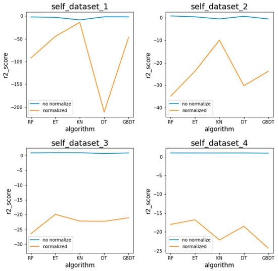
Figure 8.
Normalization experiment of the self condition.
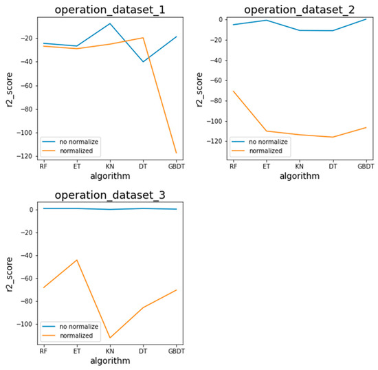
Figure 9.
Normalization experiment of the operation condition.
4.2. Training Results of the Five Machine Learning Models
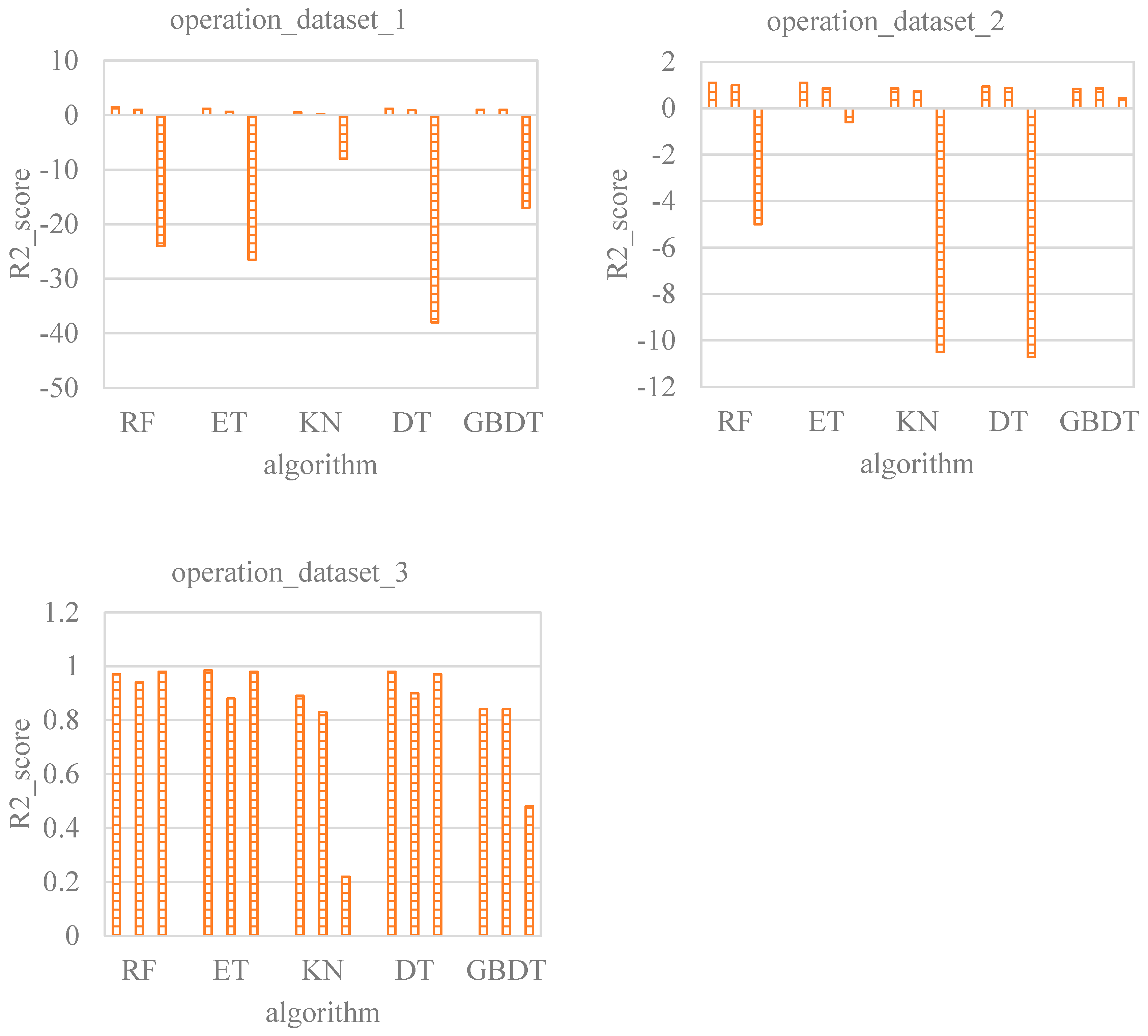
The purpose of the comparison experiments in this section is to identify the most suitable model to replace numerical calculations among the five machine learning models. The accuracy of each trained model is evaluated by r2_score, calculated based on validation and test dataset. When the predicted results are too far away from the r2_scores, the r2_score values show negative abnormally.
Figure 10 shows the comparison of different models under the self condition. Datasets 1 and 2 are sampled on the global scale, while datasets 3 and 4 add local data based on global data. Because the amount of data in dataset 1 is small, and the sampling points in the global scope are relatively sparse, the r2_score of the test dataset is all negative. Adding global data to dataset 1, the r2_score of the test datasets of RF, ET, and DT become positive (0.7706, 0.3787, and 0.6148). Although the r2_score of KN and GBDT are improved by the addition of global data, the value is still negative. After dataset 3 and dataset 4 add training data near the test points, the accuracy of all the assessed models is greatly improved. However, the histogram of data 4 indicates that the KN and GBDT models still underperform the other three models based on the r2_score.
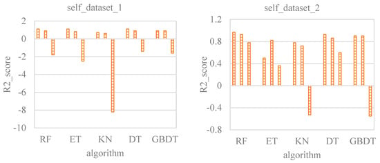
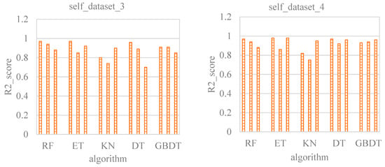
Figure 10.
Comparison of different models under the self condition.
As a result, the KN and GBDT models are first excluded, and the appropriate model is selected from the remaining three. DT shows the best performance with dataset 1, but the accuracy becomes lower than RF and ET as the dataset is expanded. Although the accuracy of ET is lower than RF and DT after the increase in local data, the performance of the validation dataset is always worse than that of RF and DT, and the performance on global data is not as good as RF and DT, indicating that ET has a higher accuracy rate depending on data density. Compared with ET, RF has the highest r2_score of the test dataset on the global data. With the addition of local data, the r2_score of the test dataset reaches 0.9999. Therefore, RF is found to be the most suitable machine learning model for the self condition.
Figure 11 shows the comparison of different models under the operation condition. Dataset 1 is the data sampled on the global scale, dataset 2 includes local data around the test points based on global data, and dataset 3 further adds local data based on dataset 2. There are few data sampled in the global scope of the operation, and the new local data in dataset 2 are also scarce. Because the operation condition has a large number of input parameters and involves complex calculations, the performance of the models trained by datasets 1 and 2 is not satisfactory. The accuracy of the model trained by dataset 3 is significantly improved due to the addition of local data. Given the poor accuracy found with the first three datasets, the KN, DT, and GBDT models are first excluded. Although the ET model outperforms the RF model with dataset 2, the relationship is not conclusive, given the small dataset size. Since the validation dataset result of the RF model is consistently better than the ET model, the RF model is regarded as the best among the five assessed machine learning models.
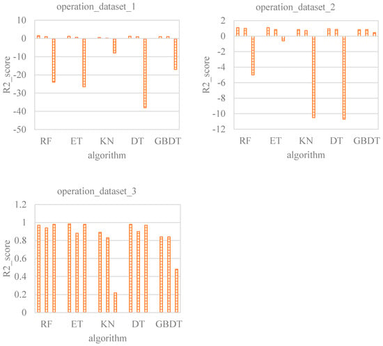
Figure 11.
Comparison of different models under the operation condition.
4.3. Relative Error of the RF Model
This section further evaluates the performance of the RF model by the relative error as defined by Equation (4). Figure 12 reflects the process in more detail from the perspective of relative error using box plots under the self condition. The closer the relative error is to 0, the closer the predicted value of the model is to the true value. The horizontal axis is the output data o1, o2, o3, and o4, which represent minlaidl, maxchainFC, maxchainFC_DNV, and maxoffsetC, respectively. The vertical axis is the relative error of the RF model calculated by each output data. The value and distribution of the relative error can be observed from the box plots. For the model trained by dataset 1, the relative error of the output data except o1 is far from 0. With the addition of a batch of global data, the relative error of the output data under dataset 2 becomes much smaller with the relative error of o1~o3 bounded by 0.2 and o4 by 0.5, and the box plot is symmetrically distributed around 0. For the model generated by dataset 3 with more local data around the test points, the absolute value of the relative errors of o1, o2, o3, and o4 is under 0.0366, 0.0985, 0.1215, and 0.0546, respectively. The relative errors of the four output data are closer to zero. Sampling more data around the test points, the absolute value of the relative error of the model trained by dataset 4 is almost 0, suggesting little deviation of the predicted output value from the true value.
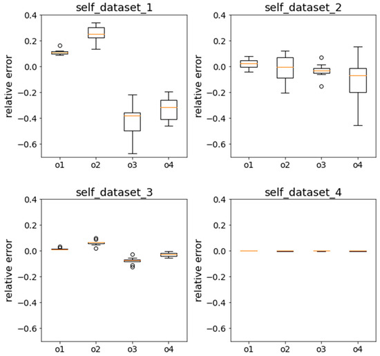
Figure 12.
Box plot of the relative error of the RF model trained by dataset 1~4 under the self condition.
Figure 13 shows the visualized relative error in a box plot for the operation condition. The horizontal axis includes one more output data from that of the self condition. o1, o2, o3, o4 and o5, respectively, represent minlaidl, max_hawserC, maxchainFC, maxchainFC_DNV, and maxoffsetC. For dataset 1 with a small amount of data and sparse distribution, the absolute value of the relative errors of o1, o3, and o5 are overall within the range of 0.5, and the relative errors of o2 and o4 are far from 0, with the values relatively scattered. The absolute value of the relative errors of the five output data on dataset 2 is mostly under 0.3. With further densification of the local data, the absolute value of the relative errors of the five output data of the model trained by dataset 3 is reduced to around 0.
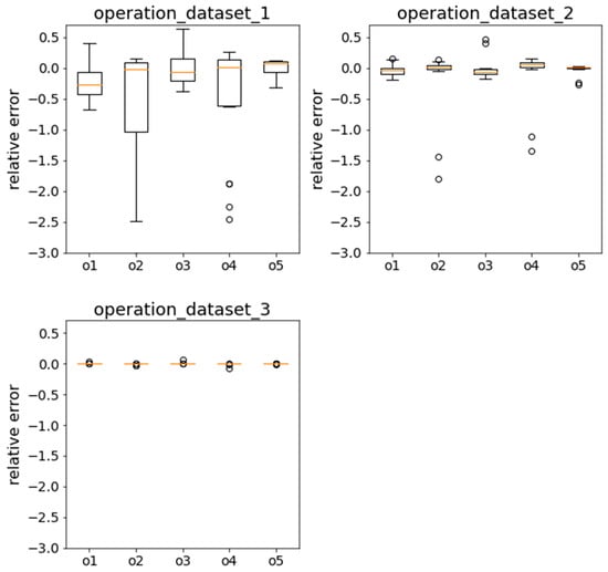
Figure 13.
Box plot of the relative error of the RF model trained by dataset 1~4 under the operation condition.
5. Conclusions
In order to explore a suitable surrogate model to replace the time-consuming numerical simulation, five machine learning models are assessed, and a sampling strategy is proposed for both global and local data considering various parameters and sampling accuracy. The machine learning models trained by different sampled datasets are qualified by both R2 and relative error under the self and operation conditions. The RF model was shown to possess the highest prediction accuracy compared to the other four models. The model’s performance could be greatly improved by the addition of local data, with the prediction asymptotically approaching the actual value as the local data density becomes higher. On top of the satisfactory accuracy, the RF model features short training time and is therefore considered to be a suitable alternative to the numerical simulation.
The emphasis of the present research is placed heavily on the effect of the local data range on model accuracy. Although the feasibility of replacing the numerical models with the RF model is proven, the amount of sampled data needs to be increased in future assessments with the guidance of the proposed sampling strategy to generate more realistic models for testing and application purposes.
Author Contributions
Study design, data analysis, and literature survey—Q.S., study design—J.Y., literature survey—D.P., figures—Z.L. and X.C., study design and guide—Y.W. All authors have read and agreed to the published version of the manuscript.
Funding
This research was funded by National Natural Science Foundation of China: US1906233, Fundamental Research Funds for the Central Universities: DUT20ZD213, DUT20LAB308.
Data Availability Statement
The data presented in this study are available upon request from the corresponding author. The data are not publicly available due to privacy.
Conflicts of Interest
Authors Qiang Sun and Dongsheng Peng were employed by the company Dalian Shipbuilding Industry Co., Ltd. Authors Jun Yan, Zhaokuan Lu and Yuxin Wang were employed by DUT. The remaining authors declare that the research was conducted in the absence of any commercial or financial relationships that could be construed as a potential conflict of interest.
References
- Ma, K.-T.; Shu, H.; Smedley, P.; L’hostis, D.; Duggal, A.S. A Historical Review on Integrity Issues of Permanent Mooring Systems. In Proceedings of the Offshore Technology Conference, Houston, TX, USA, 9 May 2013. [Google Scholar]
- Menezes, I.; Menezes, M. Genetic Algorithm Optimization for Mooring Systems. Generations 2003, 1, 3. [Google Scholar]
- Christiansen, N.H.; Voie, P.E.T.; Hgsberg, J.; Sdahl, N. Efficient Mooring Line Fatigue Analysis Using a Hybrid Method Time Domain Simulation Scheme. In Proceedings of the International Conference on Ocean, Offshore and Arctic Engineering, American Society of Mechanical Engineers, Nantes, France, 9–14 June 2013; p. V001T001A035. [Google Scholar]
- Christiansen, N.; Voie, P.; Høgsberg, J. Artificial Neural Networks for Reducing Computational Effort in Active Truncated Model Testing of Mooring Lines. In Proceedings of the International Conference on Offshore Mechanics and Arctic Engineering, American Society of Mechanical Engineers, St. John’s, NL, Canada, 31 May–5 June 2015; p. V001T001A018. [Google Scholar]
- Lin, Z.; Liu, X. Assessment of Wind Turbine Aero-Hydro-Servo-Elastic Modelling on the Effects of Mooring Line Tension via Deep Learning. Energies 2020, 13, 2264. [Google Scholar] [CrossRef]
- Lin, Z.; Liu, X. Identifying the Major Contributing Factors for Fowt Mooring Line Tension Using Artificial Neural Network. In Proceedings of the International Conference on Applied Energy 2019, Västerås, Sweden, 12–15 August 2019. [Google Scholar]
- Pillai, A.C.; Thies, P.R.; Johanning, L. Mooring system design optimization using a surrogate assisted multi-objective genetic algorithm. Eng. Optim. 2019, 51, 1370–1392. [Google Scholar] [CrossRef]
- Chen, P.; Song, L.; Chen, J.-H.; Hu, Z. Simulation annealing diagnosis algorithm method for optimized forecast of the dynamic response of floating offshore wind turbines. J. Hydrodyn. 2021, 33, 216–225. [Google Scholar] [CrossRef]
- Yetkin, M.; Mentes, A. Optimization of spread mooring systems with Artificial Neural Networks. In Towards Green Marine Technology and Transport; CRC Press: Boca Raton, FL, USA, 2015; pp. 233–238. [Google Scholar]
- Xiaoying, X.U.; Pan, Z.; Kuan, W. Mooring optimization design based on neural network and genetic algorithm. Chin. J. Ship Res. 2017, 12, 97–103. [Google Scholar]
- Li, L.; Jiang, Z.; Ong, M.C.; Hu, W. Design optimization of mooring system: An application to a vessel-shaped offshore fish farm. Eng. Struct. 2019, 197, 109363. [Google Scholar] [CrossRef]
- Panda, J.P. Machine Learning for Naval Architecture, Ocean and Marine Engineering. arXiv 2021, arXiv:2109.05574. [Google Scholar] [CrossRef]
- Yee, X.E.; Mohamed, M.A.W.; Montasir, O.A. Application of Artificial Neural Network on Health Monitoring of Offshore Mooring System. In Proceedings of the IOP Conference Series: Materials Science and Engineering, Batu Pahat, Malaysia, 1–2 December 2020; IOP Publishing: Bristol, UK, 2021; p. 012035. [Google Scholar]
- Sidarta, D.E.; Kyoung, J.; O’Sullivan, J. Prediction of offshore platform mooring line tensions using artificial neural network. In Proceedings of the International Conference on Offshore Mechanics and Arctic Engineering, American Society of Mechanical Engineers, Trondheim, Norway, 25–30 June 2017; p. V001T001A079. [Google Scholar]
- Sidarta, E.; O’Sullivan, J.; Lim, H.-J. Damage Detection of Offshore Platform Mooring Line Using Artificial Neural Network. In Proceedings of the International Conference on Offshore Mechanics and Arctic Engineering, American Society of Mechanical Engineers, Madrid, Spain, 17–22 June 2018; p. V001T001A058. [Google Scholar]
- Saad, A.M.; Schopp, F.; Barreira, R.A. Using Neural Network Approaches to Detect Mooring Line Failure. IEEE Access 2021, 9, 27678–27695. [Google Scholar] [CrossRef]
- Sidarta, D.E.; Lim, H.J.; Kyoung, J. Detection of mooring line failure of a spread-moored FPSO: Part 1—Development of an artificial neural network based mode. In Proceedings of the International Conference on Offshore Mechanics and Arctic Engineering, Glasgow, UK, 9–14 June 2019; p. V001T001A042. [Google Scholar]
- Gumley, J.M.; Henry, M.J.; Potts, A.E. A novel method for predicting the motion of moored floating bodies. In Proceedings of the International Conference on Offshore Mechanics and Arctic Engineering. American Society of Mechanical Engineers, Busan, Republic of Korea, 19–24 June 2016; p. V003T002A056. [Google Scholar]
- Chung, M.; Kim, S.; Lee, K.; Shin, D.H. Detection of damaged mooring line based on deep neural networks. Ocean Eng. 2020, 209, 107522. [Google Scholar] [CrossRef]
- Kwon, D.S.; Jin, C.; Kim, M.H.; Koo, W. Mooring-Failure Monitoring of Submerged Floating Tunnel Using Deep Neural Network. Appl. Sci. 2020, 10, 6591. [Google Scholar] [CrossRef]
- Rules for Building and Classing Single Point Moorings; American Bureau of Shipping: Houston, TX, USA, 2019.
- DNVGL-OS-E301; Position Mooring; DNV: Bærum, Norway, 2015.
- McKay, M.D.; Beckman, R.J.; Conover, W.J. A Comparison of Three Methods for Selecting Values of Input Variables in the Analysis of Output from a Computer Code. Technometrics 2000, 42, 55–61. [Google Scholar] [CrossRef]
- Gareth, J.; Daniela, W.; Trevor, H.; Robert, T. An Introduction to Statistical Learning: With Applications in R (Springer Texts in Statistics); Springer: Berlin/Heidelberg, Germany, 2013. [Google Scholar]
- Breiman, L.; Friedman, J.; Olshen, R.; Stone, C. Classification and Regression Trees; Classification and Regression Trees: Wadsworth, OH, USA; Belmont, CA, USA, 1984. [Google Scholar]
- Breiman, L. Random Forests. Mach. Learn. 2001, 45, 5–32. [Google Scholar] [CrossRef]
- Hastie, T.; Tibshirani, R.; Friedman, J. Elements of Statistical Learning; Springer: Berlin/Heidelberg, Germany, 2009. [Google Scholar]
- Zhihua, Z. Machine Learning; Tsinghua University Press: Beijing, China, 2016. [Google Scholar]
- Geurts, P.; Ernst, D.; Wehenkel, L. Extremely randomized trees. Mach. Learn. 2006, 63, 3–42. [Google Scholar] [CrossRef]
- Friedman, J.H. Greedy Function Approximation: A Gradient Boosting Machine. Ann. Stat. 2001, 29, 1189–1232. [Google Scholar] [CrossRef]
- Friedman, J.H. Stochastic gradient boosting. Comput. Stat. Data Anal. 2002, 38, 367–378. [Google Scholar] [CrossRef]
- Altman, N.S. An Introduction to Kernel and Nearest-Neighbor Nonparametric Regression. Am. Stat. 1992, 46, 175–185. [Google Scholar] [CrossRef]
Disclaimer/Publisher’s Note: The statements, opinions and data contained in all publications are solely those of the individual author(s) and contributor(s) and not of MDPI and/or the editor(s). MDPI and/or the editor(s) disclaim responsibility for any injury to people or property resulting from any ideas, methods, instructions or products referred to in the content. |
© 2024 by the authors. Licensee MDPI, Basel, Switzerland. This article is an open access article distributed under the terms and conditions of the Creative Commons Attribution (CC BY) license (https://creativecommons.org/licenses/by/4.0/).

