Development of Individual Rotor Mutual Induction (IRMI) Method for Coaxial Counter-Rotating Rotor

Abstract

A coaxial counter-rotating rotor (CCRR), which has two rotors rotating in the opposite directions on the same axis, is seen as a promising technology for low-cost floating tidal current/ocean current power generation using single-point mooring, as the torques of the front and rear rotors are cancelled. In the evaluation and design of such turbines, there is a need for an accurate analysis method with a low computational load that considers the strong mutual induction between the two rotors placed close together. An individual rotor mutual induction (IRMI) method was developed in this study, aiming to significantly reduce the calculation time of conventional computational fluid dynamics (CFD), considering the mutual induction that are not considered in conventional modified blade element and momentum methods. In this method, the basic characteristics of the front and rear rotors are calculated in advance using full-model CFD. In calculations for the CCRR, in addition to these individual characteristics of each rotor, the interaction between the rotors is considered using the actuator disk model CFD calculated in advance. The condition where the torques of the front and rear rotors are cancelled is determined at the same time. This method was used to analyze models in which the front and rear rotors were approximately the same diameter and placed close together (10% of the rotor diameter). A comparison with the mixing plane model CFD revealed that they agree quite well when mutual induction is considered, although both the power and thrust are overcalculated when it is ignored. The simulation time of the IRMI would be almost counter-proportional to the numbers of TSR conditions to solve as compared with the CFD with the MP model.

1. Introduction

As the effects of global warming have become more apparent in recent years, major countries are working toward carbon neutrality. And there are high expectations for renewable energy with low CO₂ emissions in the power generation sector. Hydro, wind, solar, and biomass have taken the lead among renewable energy sources. Although two-thirds of the Earth’s surface is covered by oceans, most ocean-based renewable energy, including tidal and ocean current power generation, is still at the demonstration stage, and it is difficult to say whether it will be put into practical use globally.

Tidal power generation is a technology that uses tidal currents to generate electricity. Since tidal level changes are a periodic phenomenon caused by the gravity of the moon, it is also easy to predict the amount of power generated by tidal current power generation. In addition, ocean current power generation is a technology that uses ocean currents. Ocean currents are generated by solar heat, westerlies, the Earth’s rotation, and the topography, and do not change significantly, so it is easy to predict the amount of power generated via ocean current power generation. Therefore, tidal current/ocean current power generation is easier to manage as part of an existing power supply system than wind and solar powers, which have already been introduced a lot.

There are two types of tidal current/ocean current turbines: the bottom fixed type, which has its base fixed to the seabed, and the floating type, which is moored with one or more mooring lines. Each has pros and cons, but, to reduce the levelized cost of energy (LCOE), floating tidal/ocean current power generation is promising because of its ability to utilize faster currents close to the water surface, ease of construction, maintainability, and ability to follow changes in the current direction—in other words, no yaw control required. Especially, single-point moored floating tidal current/ocean current turbines have the potential to significantly minimize the mooring system and its construction costs, which account for a large proportion of the initial cost.

To operate a single-point moored floating tidal current/ocean current turbine stably, the average torque acting on the mooring line must be reduced to zero. One of the technologies that makes this possible is the coaxial counter-rotating rotor (CCRR). This rotates the front rotor (FR) and rear rotor (RR) coaxially, and so they rotate in opposite directions. Several papers have reported that the power coefficient of the rotor increases slightly compared to a single rotor. However, with CCRRs, the influence of the mutual interference between the FR and RR is large, so an analysis method that takes this into consideration is required.

CCRRs are used in tidal/ocean current turbines and wind turbines, which are the subject of this research, as well as propulsion systems for aircrafts, ships, and helicopters. The characteristics of tidal/ocean currents that are relevant to wind turbines are that they are incompressible flows with open channels; the loads on each rotor are, thus, generated in almost the same plane, and the blades have a relatively large aspect ratio. The existing analysis techniques are listed below in order of fidelity. The methods for analyzing counter-rotating wind turbines are relatively well-summarized in Oprina et al. [1].

(1)

Full-model computational fluid dynamics (CFD)

The most common analysis method for CCRRs is full-model CFD, which models the rotors in one domain and analyzes it dynamically. This method has the advantage of being able to analyze rotor mutual interference and fluctuating loads even if there is misalignment between the flow direction and rotor axis or shear of the inflow. But it requires extremely huge amounts of computational resources and time. Furthermore, at least three cases of simulations are required to find the condition where the torques of the FR and RR are balanced, and so it is not realistic to apply in practical designs.

Liu et al. [2] investigated the effects of the distance between the rotors and rotor speed in the CCRR using large eddy simulation (LES). If the distance between the rotors is small, the performance of the FR decreases significantly, and, if the distance is large, the RR generates variable loads due to the wake effects of the FR. Further, if the rotation speed of the RR increases, the performance of the FR decreases significantly. In addition, turbulent regions are also generated by the blade root vortices of the FR. This also showed that a separation of 0.4 times the diameter resulted in a 10% higher efficiency than the single rotor.

Szlivka et al. [3] compared four CFD methods for CCRRs. They reported that the sliding mesh method is the most appropriate for dynamic calculation, but the mixing plane (MP) method can simulate the dynamics of the rotor appropriately. Considering the results, the MP method was used as the reference in the present research. It is explained in a little more detail in (3) below.

In addition, studies of the CCRR using full-model CFD have been undertaken by Sutikno and Saepdin [4] and Kumar [5]. There are no special notes on them as an analysis method.

(2)

CFD with actuator line model (ALM)

One of the typical approaches for the simplification of CFD is the ALM, developed by Sorensen [6]. The ALM calculates the loads on the blades based on the blade element theory. And the flow around the blades is induced by the reaction force.

Pacholczyk et al. [7] applied the ALM for the calculation of CCRR performance. No significant interference was found between the two rotors if the clearance between the two rotors is 0.5 time of the rotor diameter (D), which is significantly larger than the CCRR in the present study (0.1 D).

(3)

CFD with mixing plane (MP) model

The MP model transfers the interaction between two numerical regions. The application of the present model is limited for a steady symmetric flow [7], which is assumed in the present study. Each of the FRs and RRs is represented by one blade, periodic boundary conditions are applied in the rotation direction, and the interaction between the two rotors is transmitted at the radial position of each blade [8]. Since the interaction between the rotors is averaged in the azimuth, it is not theoretically possible to analyze the dynamic characteristics as obtained by full-model CFD. However, it has been reported that analyses of the average load can be undertaken with good agreement. Even with this method, three or more calculations are required for each condition to find the point where the torque is balanced, but the analysis time can be significantly reduced in accordance with the number of blades. However, this method is limited when applied to axially symmetrical airflow and for average loads.

Details of this method are shown in Section 4.

(4)

Vortex lattice method

Lee et al. [9] compared single rotors and the CCRR using the vortex lattice method. They reported that the axial induction coefficient increases as the solidity increases, and the axial induction coefficient of the CCRR is lower than that of the single rotor. The maximum power coefficient of the CCRR is approximately 30% higher than that of the single rotor. A verification of this method was not conducted for the CCRR, but only for a single rotor.

In addition, Lee et al. [10] conducted an analysis using the free-wake vortex lattice method, considering the effects of the mutual interference between the FR and RR. The induction coefficient of RR was compared with that of the blade element and momentum (BEM) method, assuming that the RR is completely within the wake of FR; that is, the influence of the RR on FR is not considered.

(5)

Blade element and momentum (BEM) method

Lee et al. [11] developed a modified BEM method and investigated the influence of the design parameters on the CCRR. This method considers the interaction of the FR with RR as a flow within a well-developed wake but does not consider the interaction of the RR with FR. Note that the torque balance between both rotors is taken into consideration.

Furthermore, Hwang et al. [12] used the same method to evaluate the power and thrust coefficients using the pitch angle, diameter ratio, and rotor speed of the CCRR as variables.

Note that some of these studies are related to the CCRR, which was developed in South Korea around 2010, which has an FR diameter that is 1/2 that of the RR, and the inboard sections of the RR blades are not expected to generate torque. In addition, both the rotors are located at the front and rear of the nacelle, and the distance between rotors is relatively large. In these modified BEM methods, the interaction of the FR with RR is treated as a fully developed wake flow, and the interaction of the RR with FR is ignored. Therefore, it is necessary to verify the reliability of the method for CCRRs in which the FR and RR are relatively close to each other and have almost the same diameter.

(6)

CFD with actuator disk model (ADM)

Newman [13] investigated the characteristics of a tandem rotor using a one-dimensional ADM that ignores swirling flow, with the aim of applying it to vertical axis wind turbines. The results show that the power coefficient increased by 18% compared to that for a single rotor at the Betz limit. Of course, this method is not applicable for blade design.

In the design of floating tidal current/ocean current turbines, a high accuracy and low analysis load are required for the fluid dynamics analysis. Among the above methods, the conventional (1) full-model CFD, (2) ALM, and (3) MP model can be used to comprehend many phenomena, but it is difficult to use them for an actual motion/response analysis due to the heavy load required in calculation. On the other hand, the conventional (5) modified BEM is not acceptable when it is applied to the CCRR which the diameters of FR and RR are same, and for which the rotors are placed close together.

Considering the above, individual rotor mutual induction (IRMI) was developed for use on the CCRR based on the fluid force characteristics of the individual rotors. This eliminates the need for calculations seeking to find the balance point between the torques of the FR and RR, which is required in conventional analysis methods (1) and (2). It can handle mutual induction, and the analysis time can be significantly reduced while maintaining analysis accuracy.

Section 2 provides an overview of the analysis method, Section 3 provides the case study model, and Section 4 provides the steady-state CFD results for the MP model CCRR for verification. Section 5 and Section 6 present the CFD results for individual rotors and the mutual induction factors. Section 7 shows the analysis results using the IRMI method developed in this research. Then, Section 8 summarizes the research overall.

2. IRMI Method

Figure 1 shows the flowchart of the present IRMI method. The yellow shading in the figure concerns calculations performed using the individual rotor characteristics in Section 2.1 and the mutual induction factors in Section 2.2 (Mutual Induction Factors), calculated by CFD in advance. The gray shading shows the input condition in Section 2.3. The dashed array and thick array show the mutual induction and the equal torque, respectively. And the numbers in the chart are the numbers of equations shown in Section 2.4.

Note that this analysis method only deals with a uniform flow parallel to the rotor axis.

2.1. Characteristics of the Individual Rotor

The characteristics of the thrust coefficient C_T, power coefficient C_P, and torque coefficient C_Q for the TSR λ are determined in advance. They were calculated using CFD in this study, but, in principle, other analytical methods or experimental values can be used instead.

2.2. Mutual Induction Factors

This research proposes the mutual induction factors b as the following formula, inspired by the axial induction factor a in the momentum theory or BEM:

$$\begin{array}{c}{b}_F=1-u_F\\ b_R=1-u_R\end{array}$$

(1)

where u_F and u_R are the induced velocities U_I at each rotor, normalized by the free stream (FS) velocity U as given below:

$$\begin{array}{c}{u}_F=U_{FI}/U\\ u_R=U_{RI}/U\end{array}$$

(2)

a in the momentum theory represents the induction by the rotor itself. In contrast, b represents the deceleration of the flow induced by the neighboring rotor. The b and u are the rotor plane averaged values, defined by the thrust coefficient of the neighboring rotor.

The FS velocity U is replaced by the induced velocities U_I, and the TSRs λ are replaced by the induced TSRs λ_I in the following formulation.

2.3. Condition

Define the following parameters as input conditions:

• Free stream (FS) flow velocity—U;
• FR angular speed—Ω_F.

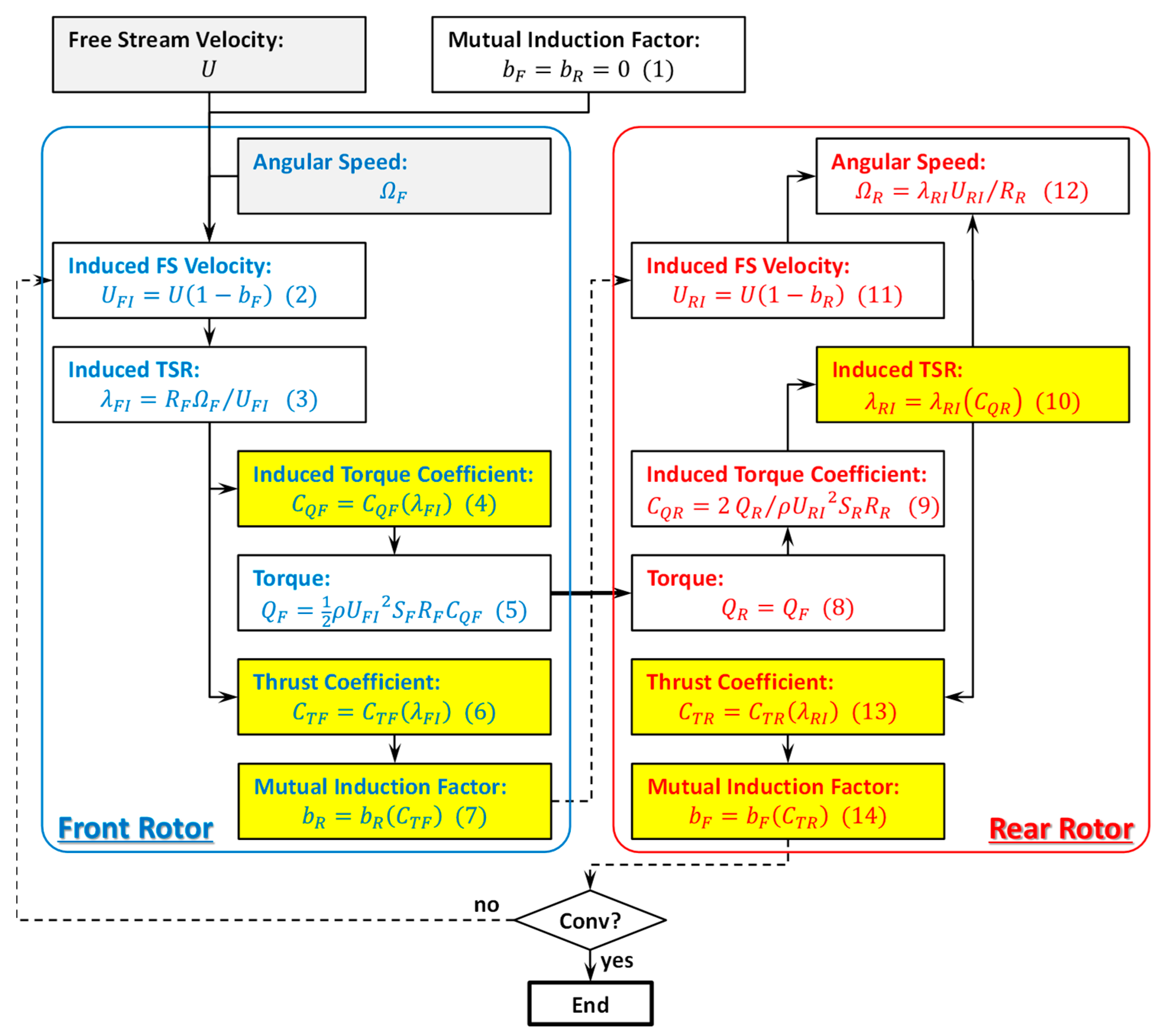
2.4. Calculation of Equilibrium Condition

To find the equilibrium conditions, the following steps are repeated until convergence, as shown in Figure 1.

(1)

Initial conditions

The initial value of the mutual induction coefficients is defined as below.

$$b_F=b_R=0$$

(3)

(2)

Induced FS velocity and induced TSR at FR

The velocity at the FR is induced not only by the FR but also by the RR as shown above. The induction of the RR, which is not considered in the individual rotor CFD, is calculated by the ADM results. The FS velocity is replaced by the induced velocity as below.

$$U_{FI}=U(1-b_F)$$

(4)

And the TSR is replaced by the induced TSR as below.

$${\lambda }_{FI}=R_F{\Omega }_F/U_{FI}$$

(5)

(3)

Torque and thrust coefficients of FR

The torque and thrust coefficients of the FR are calculated by the individual rotor CFD results at the induced TSR as following equations.

$$C_{QF}=C_{QF}\left({\lambda }_{FI}\right)$$

(6)

$$C_{TF}=C_{TF}\left({\lambda }_{FI}\right)$$

(7)

(4)

Torques of FR and RR

The torque of the FR is calculated as below by the torque coefficient in Equation (6) and induced FS velocity in Equation (4).

$$Q_F=\frac{1}{2}\rho {U_{FI}}^2{S}_F{R}_F{C}_{QF}$$

(8)

The torque of the RR is set to be the same value as the FR’s as

$$Q_R=Q_F$$

(9)

(5)

Mutual induction factor and induced FS velocity at RR

The mutual induction factor from the FR to the RR is calculated by the ADM results and the thrust coefficient of the FR by using the ADM results and the thrust coefficient of the FR as below.

$$b_R=b_R\left(C_{TF}\right)$$

(10)

The FS velocity is replaced by the induced FS velocity as below at the RR.

$$U_{RI}=U(1-b_R)$$

(11)

(6)

Torque coefficient of RR

The torque coefficient of the RR is calculated as below by the torque in Equation (9) and the induced FS velocity in Equation (11).

$$C_{QR}=2Q_R/\rho {U_{RI}}^2{S}_R{R}_R$$

(12)

(7)

Induced TSR and angular speed of RR

The induced TSR is calculated by the individual rotor CFD result as below, by using the torque coefficient of the RR in Equation (12).

$${\lambda }_{RI}={\lambda }_{RI}\left(C_{QR}\right)$$

(13)

And the angular speed is calculated as below using the induced TSR and the induced FS velocity in Equations (13) and (11).

$${\Omega }_R={\lambda }_{RI}{U}_{RI}/R_R$$

(14)

(8)

Thrust coefficient of RR

The thrust coefficient of the RR is calculated as below by the individual rotor CFD results and the induced TSR in Equation (13).

$$C_{TR}=C_{TR}\left({\lambda }_{RI}\right)$$

(15)

(9)

Mutual induction factor at FR

The mutual induction factor at the FR is calculated by the ADM results as below using the thrust coefficient of the RR in Equation (15).

$$b_F=b_F\left(C_{TR}\right)$$

(16)

The mutual induction factor is applied for Equation (4) to consider in the induction of the RR tor the induced speed at the FR.

(10)

Convergence judgment

Repeat the above calculation until the above parameters converge. Once converged, the thrust, torque, and power coefficients of the two rotors are obtained as well as the operation point, and the mutual induction factors.

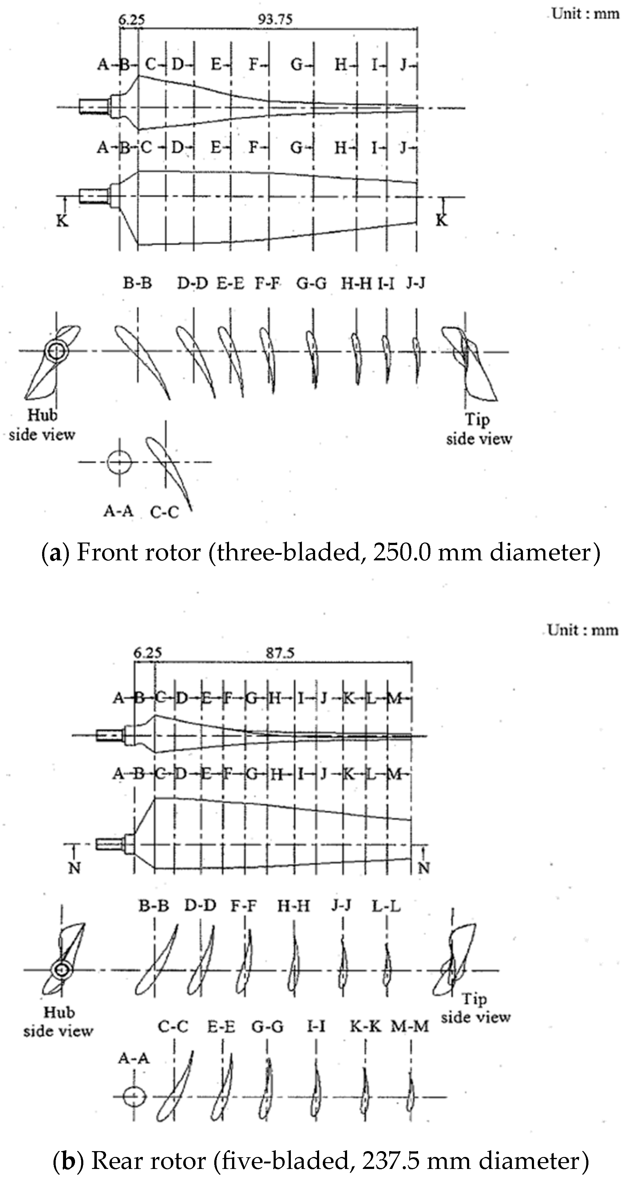
3. CCRR Model

3.1. Blade Shape

Figure 2 shows the shapes of the FR and RR blades. The cross-sectional shape of these blades is depicted by the MEL002 airfoil [14], which has excellent characteristics in low-Reynolds-number regions.

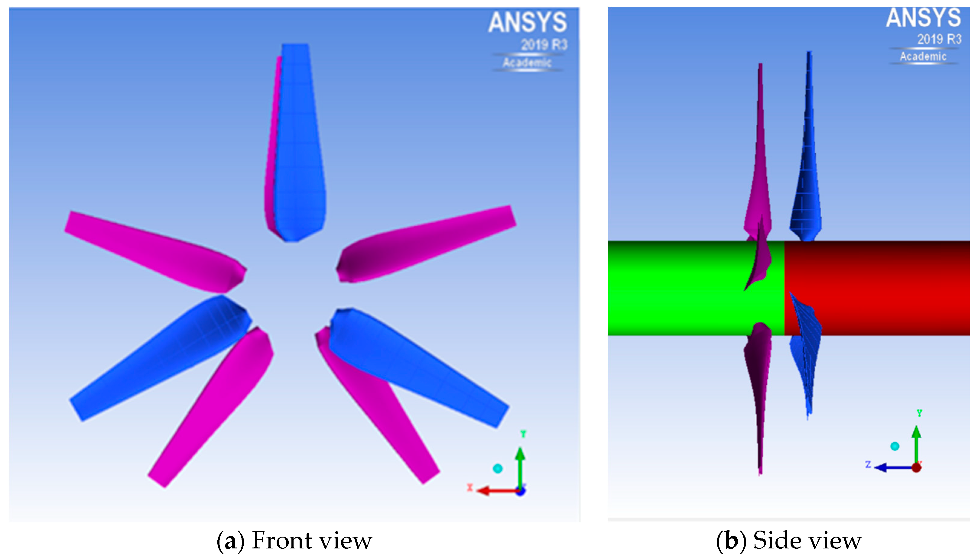
3.2. Rotor Shape

The FR used in this study has three blades with a diameter D_F = 250.0 mm, and the RR has five blades with a diameter D_R = 237.5 mm. The separation between the two rotor surfaces is 25 mm (=0.1D_F). Figure 3 shows the appearance of the CCRR.

4. CCRR MP Model CFD

This section provides an overview of the steady-state CFD of the CCRR-integrated model used for the verification of this research. The results of the analysis are shown in Section 7 in comparison with the IRMI.

4.1. Analysis Method

The commercial code ANSYS CFX (2019R3) was used to perform CFD using the MP model. The multi-reference frame (MRF) was used to handle the uniform and steady flow parallel to the rotor axis. This can be calculated in a fan-shaped domain for one blade of each rotor, taking symmetry into account. However, in the case of the CCRR, the number of blades and the rotation direction of the front and rear rotors are different, so normal MRF calculations using a single object cannot be performed. The analysis was performed on the assumption that the physical quantities of the azimuth average are the same in the annular region at the same radial position at the boundary between both rotors, in this study. According to Fuchiwaki [8], this method was compared with the experimental results elucidated by Wei et al. [15], and, although there was a difference of about 10% in the peak value, they found the TSR at which the power coefficient is maximized and the overall trend, etc. It has been reported that these findings are generally reproducible.

With this method, the analysis domain is reduced in inverse proportion to the number of blades, so the analysis time can be significantly reduced. However, after fixing the FR rotor speed, it is necessary to calculate the RR rotation speed three to five times until the torques of the FR and RR are almost equal.

4.2. Analysis Conditions

• Working fluid: water;
• Density ρ: 997 kg/m³;
• Inlet flow velocity U: 1.0 m/s;
• TSR λ: 1.0 to 8.0;
• Turbulence model: k-ω SST.

4.3. Analysis Grid/Boundary Conditions

• Wall boundary conditions: stick (blade and hub) and slip (shroud);
• Inlet boundary: flow velocity (steady);
• Outlet boundary: gauge pressure (0 Pa);
• Boundary condition between rotors: stage (mixing plane);
• Number of calculation grids: 3.6 million (front) and 3.1 million (rear);
• Analysis domain:

  Table 1. CFD for the CCRR with the MP method.

  Parameters	Values
  $\mathrm{Diameter} \mathrm{of} \mathrm{FR} D_F$ (mm)	250.0
  Center angle of the FR domain (degree)	120
  Diameter of RR $D_R$ (mm)	237.5
  Center angle of the RR domain (degree)	72
  $\mathrm{Ratio} \mathrm{of} D_R/D_F$	0.95
  Length of analysis domain (mm)	2500
  Length of analysis domain (mm)	625
  Distance between FR and RR (mm)	25

  and Figure 4.

Note that the validity of the analytical grid is explained in Fuchiwaki [8], so it is omitted here.

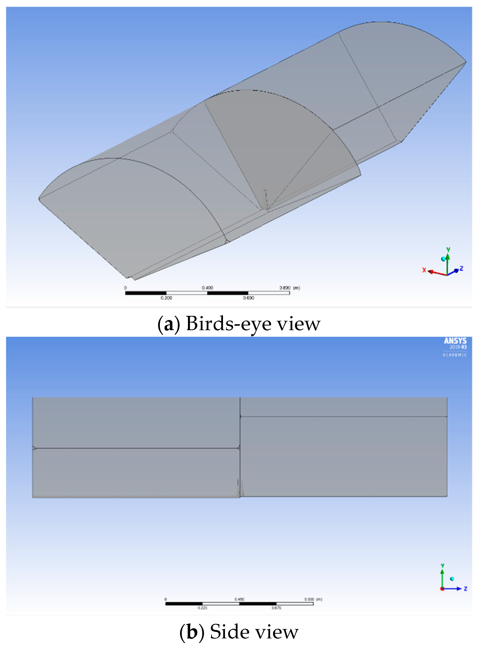
5. Individual Rotor CFD

This section presents the contents and results of analysis of CFD for the FR and RR individually, which serve as the input information for the IRMI.

5.1. Analysis Method

ANSYS CFX (2019R3) was used for the analysis. The steady characteristics in steady wind were calculated for one FR blade and one RR blade using the MP model, assuming periodical boundary conditions.

5.2. Analysis Conditions

• Working fluid: water;
• Water density ρ: 997 kg/m³;
• Inlet flow velocity U: 1.0 m/s;
• Outlet gauge pressure: 0 Pa;
• TSR λ: 1.0 to 8.0 (

  Table 2. Conditions for the individual rotor CFD.

  $\mathit{\lambda } (-)$	${\mathsf{\Omega }}_{\mathit{F}} (\mathbf{r}\mathbf{a}\mathbf{d}/\mathbf{s})$	${\mathit{n}}_{\mathit{F}} \left(\mathbf{r}\mathbf{p}\mathbf{m}\right)$	${\mathsf{\Omega }}_{\mathit{R}} (\mathbf{r}\mathbf{a}\mathbf{d}/\mathbf{s})$	${\mathit{n}}_{\mathit{R}} \left(\mathbf{r}\mathbf{p}\mathbf{m}\right)$
  1.0	−8.00	−76.39	8.42	80.42
  2.0	−16.00	−152.79	16.84	160.83
  3.0	−24.00	−229.18	25.26	241.25
  4.0	−32.00	−305.58	33.68	321.66
  5.0	−40.00	−381.97	42.11	402.08
  6.0	−48.00	−458.37	50.53	482.49
  7.0	−56.00	−534.76	58.95	562.91
  8.0	−64.00	−611.15	67.37	643.32

  );
• Turbulence model: k-ω SST.

5.3. Analysis Grid and Analysis Conditions

• Analysis domain: Figure 5;
• Wall boundary conditions: stick (blade and hub) and slip (shroud);
• Number of calculation grids: 4.1 million (FR) and 3.5 million (RR).

Figure 6 shows the mesh near the airfoil. The validity of the analytical grid is reported in Fuchiwaki [8].

Figure 5. CFD domains for the individual rotor CFD.

Figure 5. CFD domains for the individual rotor CFD.

Figure 6. Mesh around the blade section.

Figure 6. Mesh around the blade section.

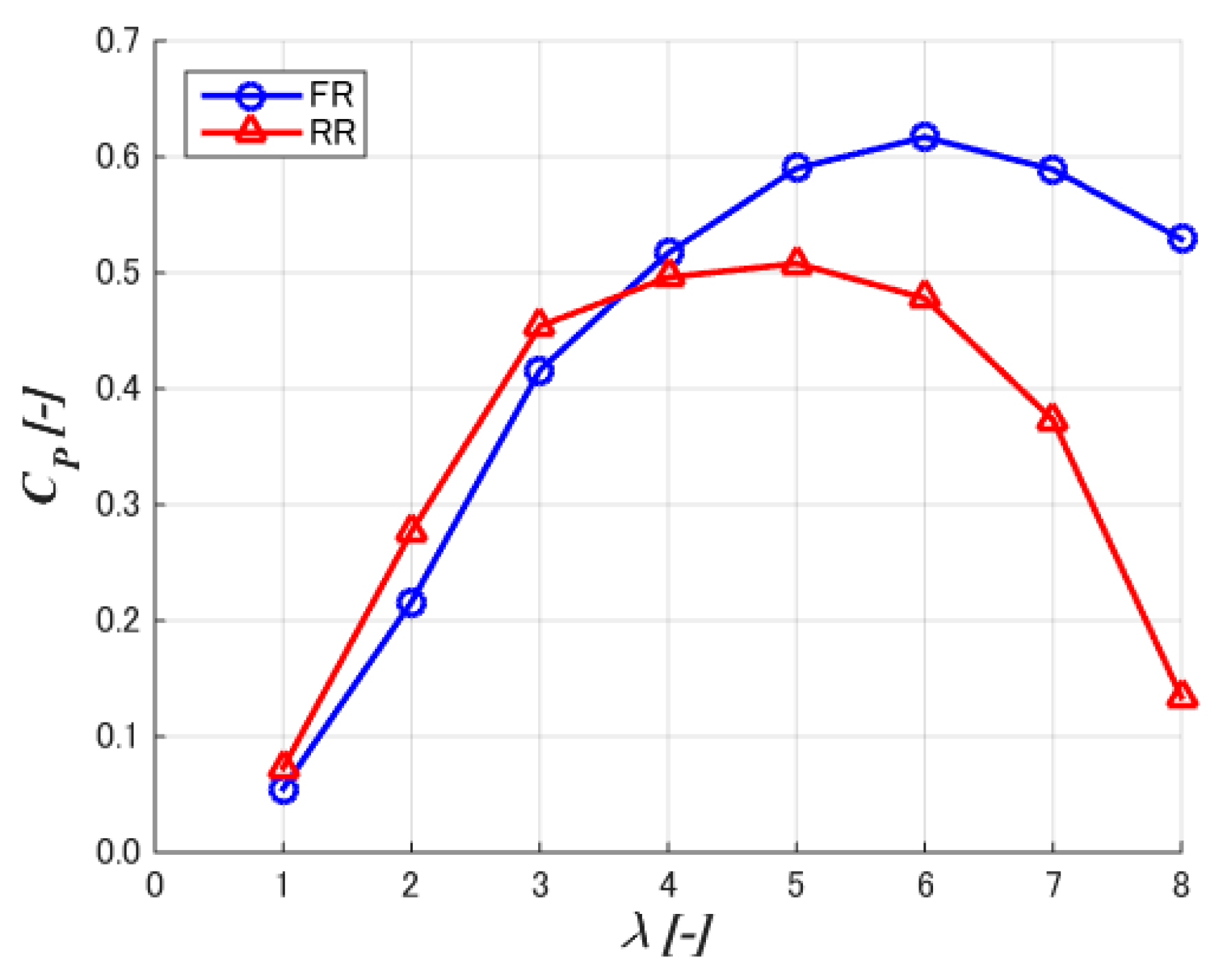
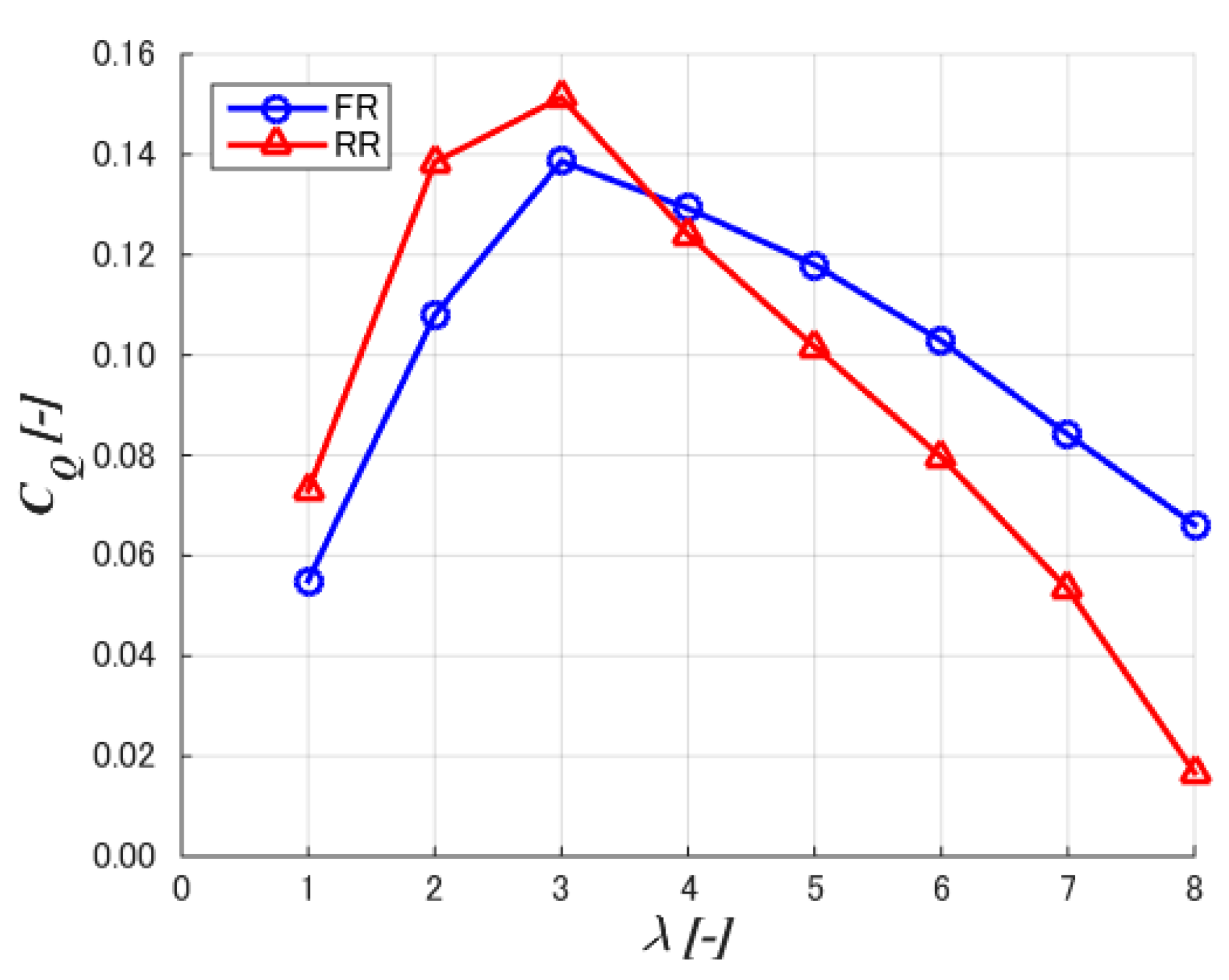
5.4. CFD Results

Figure 7, Figure 8 and Figure 9 show the thrust, power, and torque coefficients with respect to the TSR of each rotor. Since the solidity of the FR is smaller, the thrust coefficient of the FR is lower than that of the RR overall. The power coefficient is higher in the high-TSR range and lower in the low-TSR range. Furthermore, in both cases, the slope of the torque coefficient with respect to the TSR is negative when the TSR is 3 or higher.

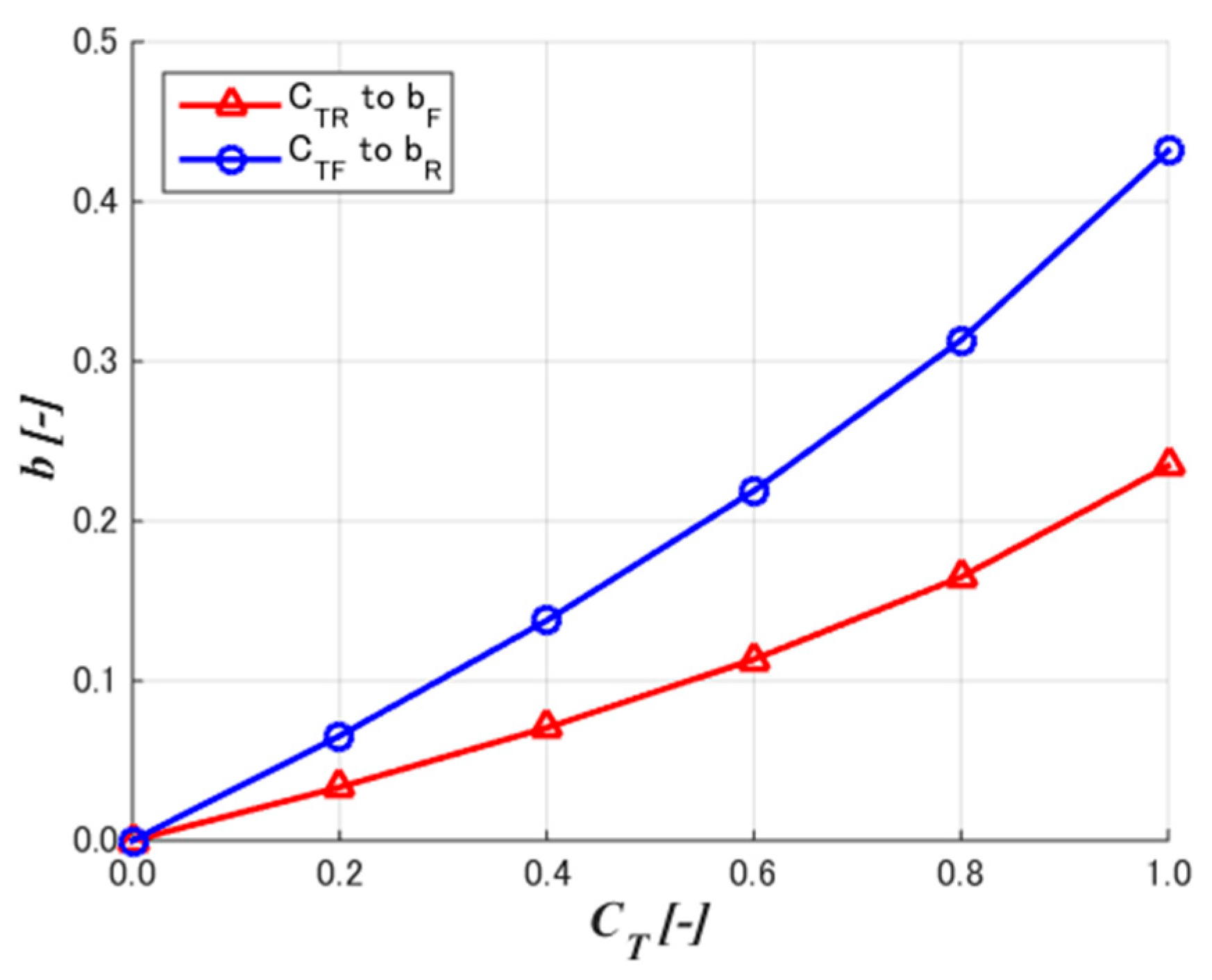
6. Mutual Induction Factors Calculation

This section presents the content and analysis results of CFD regarding the mutual induction factors between FR and RR, which serve as the input information for the IRMI.

6.1. Analysis Method

The commercial CFD software ANSYS Fluent (2023R1) was used for the analysis. The rotor was modeled by the ADM with a uniform load to calculate the steady mutual induction in steady uniform wind in this study.

6.2. Analysis Conditions

• Working fluid: water;
• Water density ρ: 997 kg/m³;
• Inlet flow velocity U: 1.0 m/s;
• Outlet gauge pressure: 0 Pa;
• Thrust coefficient C_T: 0.2 to 1.0 (0.2 each);
• Turbulence model: k-ω SST.

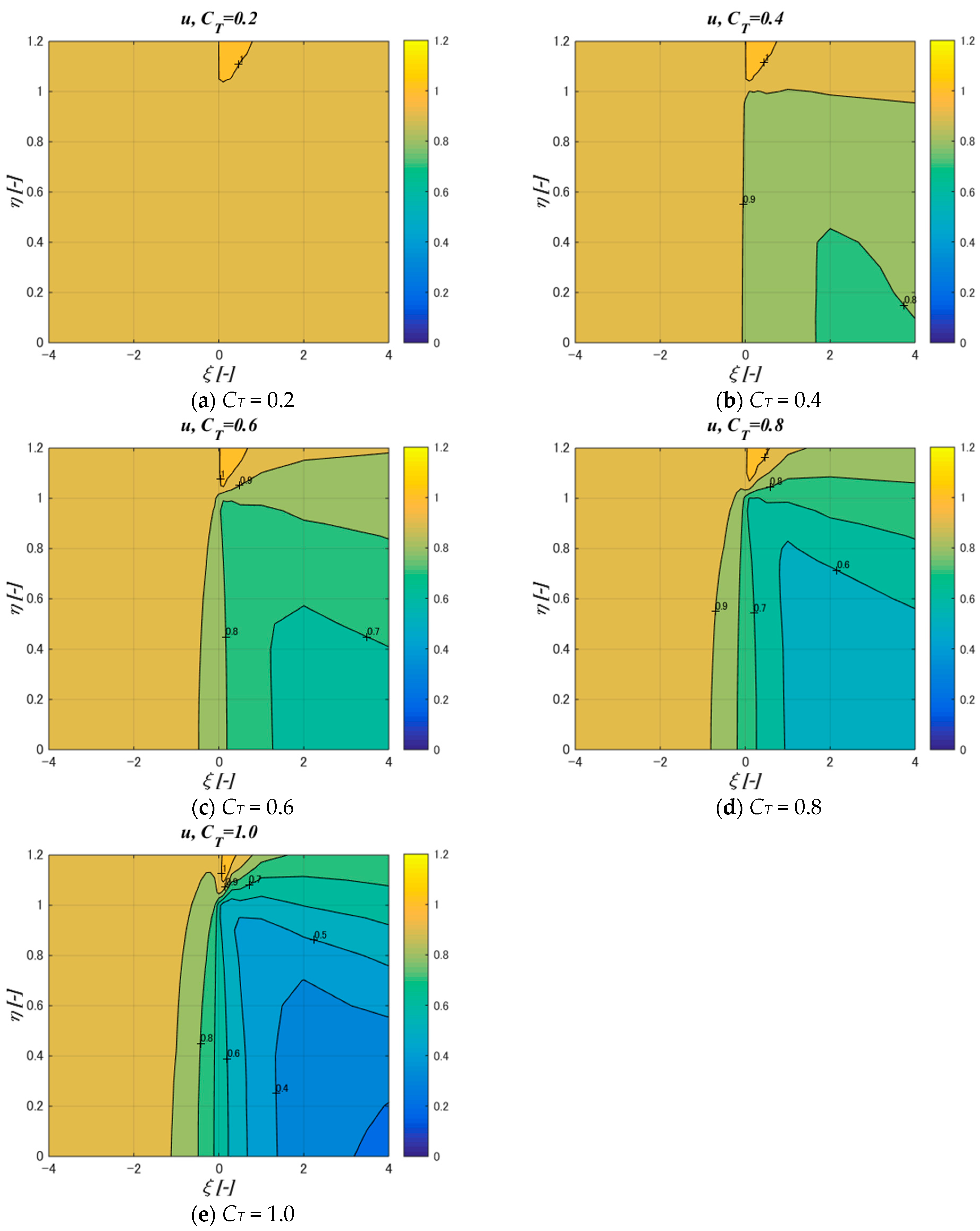
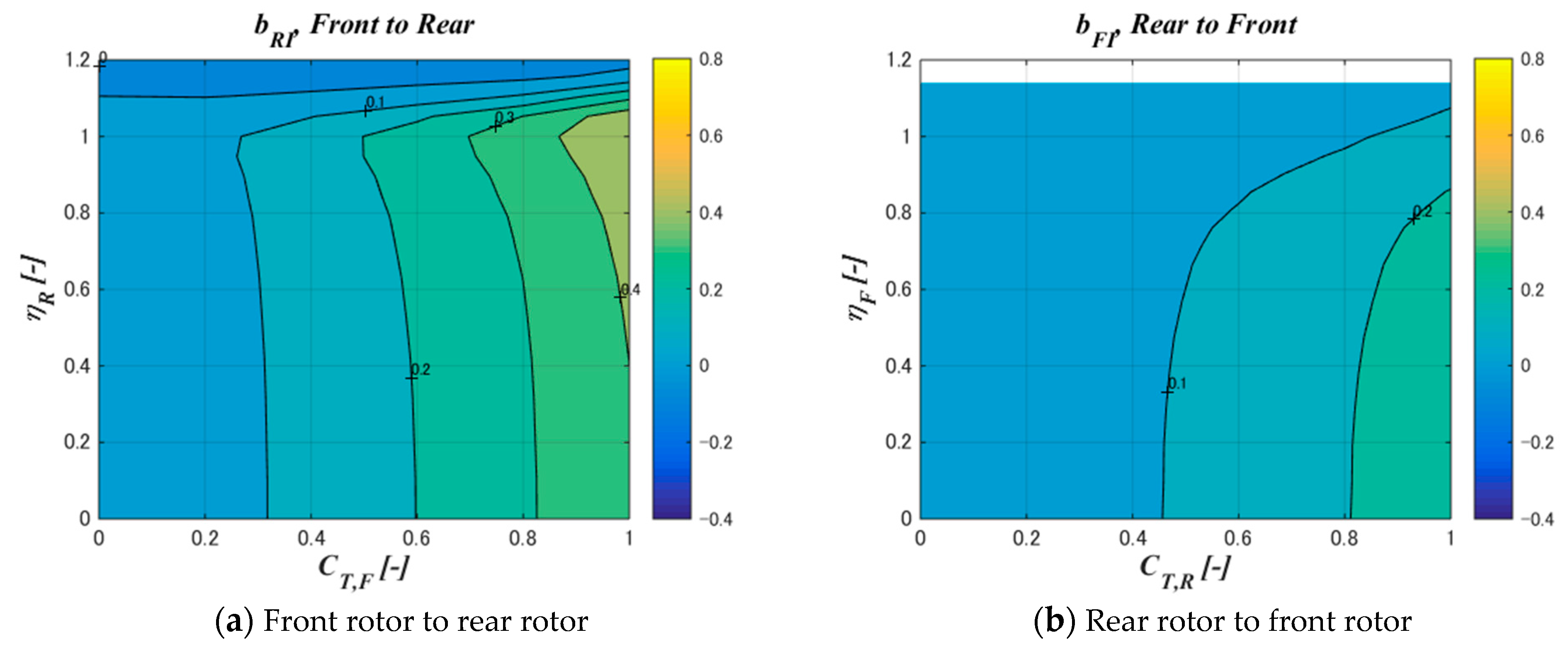
6.3. Rotor Mutual Induction Analysis Results

Figure 10 shows the normalized induced velocity around the actuator disk at typical thrust coefficients. Here, ξ is the longitudinal position normalized by the rotor diameter (ξ = x/D), with ξ = 0 at the rotor. η is the radial position normalized by the rotor radius (η = r/R), with η = 0 and η = 1 are at the center and the tip, respectively. The larger the thrust coefficient, the higher the induced velocity.

Figure 11 shows the radial distribution of the mutual induction factors, (a) FR to RR and (b) RR to FR. Here, η_F and η_R are radial positions normalized by the diameters of the FR and RR, respectively. The mutual induction factors averaged on the rotor shown in Figure 12 are used in the present method. Here, the effect of FR on RR is about twice as large as the induction caused by RR on FR.

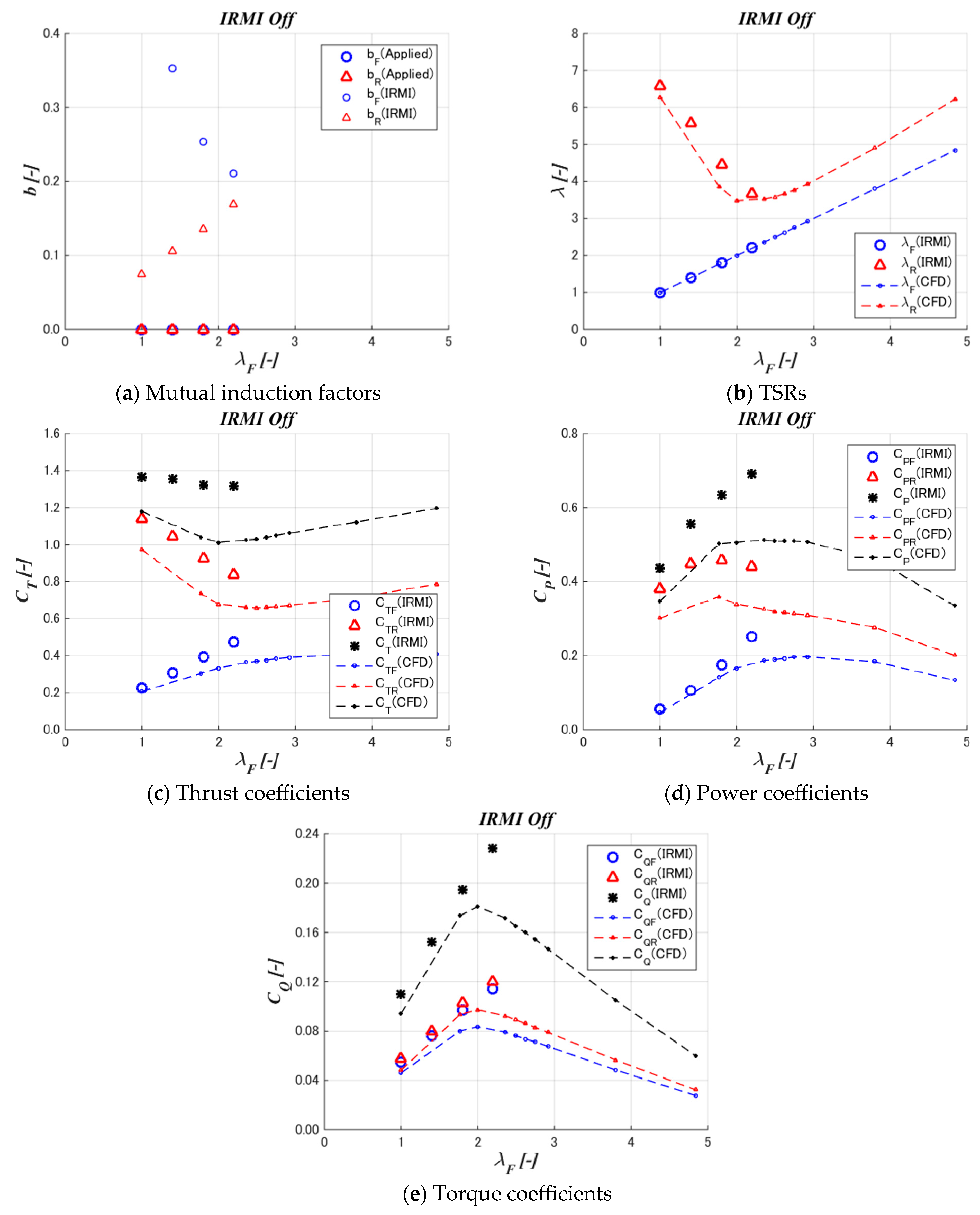
7. IRMI Method

In this section, the analysis results using the IRMI method is verified by comparing them with the MP model CFD results in Section 4.

7.1. Analysis Method

The analysis method is that shown in Section 2. Here, the data shown in Figure 7 and Figure 9 in Section 5 were used to define the characteristics of individual rotors, and those in Figure 12 in Section 6 were used for the characteristics of the mutual interference between rotors.

An example of the convergence status of the solution using the IRMI method is shown in Figure 13. In this example, the calculation is repeated 10 times, and it converges well. The dashed lines in the figure indicate the range of the CFD data.

7.2. Analysis Results

(1)

Effect of mutual interference on hydrodynamic characteristics

Figure 14 shows the analysis results with the effect of the mutual interference ignored by setting b = 0. Under this condition, the equilibrium point is simply determined by the torque characteristics of each individual rotor in Figure 9.

This analysis does not consider the deceleration caused by the thrust of the neighboring rotor, so the rotor speed (or TSR) is high. Therefore, under conditions where the TSR of the FR is approximately 2 or less, the torque and thrust coefficients are generally higher than those of the MP model CFD due to the higher TSR.

The analysis results considering the mutual induction factor, which is the original IRMI, are shown in Figure 15 together with the CFD results from Section 4. This condition considers the inherent mutual induction between the rotors, and the thrust of the FR reduces the speed of the RR by 4% to 12%, while the RR reduces the speed of the FR by 12% to 39%. When considering the mutual induction factor, the rotational speed (or TSR) of the RR decreases compared to when it is ignored. As a result, each aerodynamic coefficient is reduced, and the results are almost consistent with those of the MP model CFD.

As shown in Figure 8, the TSR at which the maximum power coefficient of each individual rotor is obtained is approximately 6 for the FR. Even in the CCRR, the power coefficient of the FR tends to increase as the TSR increases, but the power coefficient of the RR tends to decrease from around 1.5, and the power coefficient of the CCRR saturates around 1.7. This is because, as the TSR increases, the thrust coefficient also increases (Figure 7), which increases the mutual induction factor. Therefore, overall, the TSR is significantly lower than in the case of a single rotor.

(2)

Control

Another important finding in this research is the control of generators. When a single rotor is operated at a rotor speed (or TSR) that maximizes the power coefficient under a constant wind speed, if the rotor speed increases/decreases due to some disturbance, the torque decreases/increases as shown in Figure 9. The rotor speed returns to the equilibrium point in both cases. Therefore, the generator can be controlled by the torque relative to the rotational speed, and the fluctuations in the torque are small. However, in the case of the CCRR, when operating at a TSR of approximately 2, where the power coefficient is maximized, the torque will also increase/decrease as the rotational speed increases/decrease, so the above control is not possible. In this case, it is necessary to control the rotation speed at a constant value or to a set value using other parameters such as the flow velocity, instead of controlling the rotation speed with the torque. In this case, the instability in the rotational direction of the CCRR is suppressed by controlling the generator’s torque, resulting in large fluctuations in the torque or output power. This is undesirable from the viewpoint of the variation of the power and loads.

(3)

Analysis time

As mentioned in Section 4, three to five different conditions are required to calculated for one specific equilibrium condition to balance the torques of the two rotors in CFD with the MP model. On the other hands, the present IRMI method needs CFD with the MP model for the individual rotor and CFD with the ADM for the mutual induction in advance, and the calculation time to find the balanced point is as short as negligible. Therefore, the total amount of time for the IRMI is not dependent on the number of cases, but almost constant, almost the same as one case by the CFD with the MP model for the CCRR. It means, the simulation time of the IRMI would be almost counter-proportional to the numbers of TSR conditions to solve as compared with the CFD with the MP model.

8. Conclusions

8.1. Results Summary

The present IRMI method was developed for a steady load analysis for CCRRs. This method is based on the characteristics of the FR and RR individually, and the mutual induction factor between the rotors based on the ADM. It calculates characteristics such as the thrust and torque.

The analysis of the characteristics of a CCRR with a three-bladed FR and five-bladed RR during steady uniform flow revealed that, when the interference is ignored, the values are generally higher than those of CFD. It was confirmed that the results generally agree with the CFD results when considering mutual induction.

In general, for CFD, it is necessary to analyze three to five conditions in one case to find the conditions under which the torques of the FR and RR are balanced. Therefore, the present IRMI method can significantly shorten the analysis time. In this way, in the conventional method, the analysis time increases as the number of analysis cases increases, but, with the present IRMI method, although a certain amount of analysis time is required for preparation, once the preparation is completed, the analysis time hardly changes, so the analysis time increases considerably. This method is suitable for calculating large numbers.

8.2. Future Challenges

The following issues continue to persist:

(1)

The reason for the slight difference from CFD with the MP model can be that the mutual induction is assumed to be uniform on the rotor surface and the mutual induction in the rotational direction and their propagation are ignored.

(2)

The accuracy of the present method should be validated by experiments, as well as the influences of turbine configurations, such as the number of blades and the distance between the rotors.

(3)

Furthermore, the BEM theory may also be applicable to the characteristics of the individual rotor.

(4)

This study dealt with steady characteristics, which are useful for the performance and steady load. However, this method is insufficient for the application to fatigue loads, noise, etc., which are important dynamic characteristics.

References

- Oprina, G.C.; Chihaia, R.A.; El-Leathey, L.A.; Nicolaie, S.; Babutanu, C.A.; Voina, A. A Review on Counter-Rotating Wind Turbines Development. J. Sustain. Energy 2016, 7, 3. [Google Scholar]
- Liu, X.; Feng, B.; Liu, D.; Wang, Y.; Zhao, H.; Si, Y.; Zhang, D.; Qian, P. Study on Two-Rotor Interaction of Counter-Rotating Horizontal Axis Tidal Turbine. Energy 2022, 241, 122839. [Google Scholar] [CrossRef]
- Szlivka, F.; Hetyei, C.; Fekete, G.; Molnár, I. Comparison of Mixing Plane, Frozen Rotor, and Sliding Mesh Methods on a Counter-Rotating Dual-Rotor Wind Turbine. Appl. Sci. 2023, 13, 8982. [Google Scholar] [CrossRef]
- Sutikno, P.; Saepdin, D.B. Design and Blade Optimization of Contra Rotation Double Rotor Wind Turbine. Int. J. Mech. Mech. Eng. 2011, 11, 115301-7474. [Google Scholar]
- Kumar, P.S.; Bensingh, R.J.; Abraham, A. Computational Analysis of 30 kW Contra Rotor Wind Turbine. Int. Sch. Res. Netw. Renew. Energy 2012, 2012, 939878. [Google Scholar] [CrossRef]
- Sorensen, J.N.; Shen, W.Z. Numerical Modeling of Wind Turbine Wakes. ASME J. Fluids Eng. 2002, 124, 393–399. [Google Scholar] [CrossRef]
- Pacholczyk, M.; Karkosiński, D. Parametric Study on a Performance of a Small Counter-Rotating Wind Turbine. Energies 2020, 13, 3880. [Google Scholar] [CrossRef]
- Fuchiwaki, H. Development of Individual Rotor Mutual Interaction Method for Counter Rotating Rotor. Master’s Thesis, Saga University, Saga, Japan, 2024. (In Japanese). [Google Scholar]
- Lee, S.; Kim, H.; Lee, S. Analysis of Aerodynamic Characteristics on a Counter-Rotating Wind Turbine. Curr. Appl. Phys. 2010, 10, S339–S342. [Google Scholar] [CrossRef]
- Lee, N.J.; Kim, I.C.; Kim, C.G.; Hyun, B.S.; Lee, Y.H. Performance Study on a Counter-Rotating Tidal Current Turbine by CFD and Model Experimentation. Renew. Energy 2015, 79, 122–126. [Google Scholar] [CrossRef]
- Lee, S.; Kim, H.; Son, E.; Lee, S. Effects of Design Parameters on Aerodynamic Performance of a Counter-Rotating Wind Turbine. Renew. Energy 2012, 42, 140–144. [Google Scholar] [CrossRef]
- Hwang, B.; Lee, S. Lee Soogab, Optimization of a Counter-Rotating Wind Turbine Using the Blade Element and Momentum Theory. J. Renew. Sustain. Energy 2013, 5, 052013. [Google Scholar] [CrossRef]
- Newman, B.G. Multiple Actuator—Disc Theory for Wind Turbines. J. Wind. Eng. Ind. Aerodyn. 1986, 24, 215–225. [Google Scholar] [CrossRef]
- Matsumiya, H.; Kogaki, T.; Takahashi, N.; Iida, M.; Waseda, K. Development and Experimental Verification of the New MEL Airfoil Series for Wind Turbines. In Proceedings of the JWEA Symposium 2000, Tokyo, Japan, 16–17 November 2000; The International Molinological Society: Berryville, VA, USA, 2000; pp. 92–95. (In Japanese). [Google Scholar]
- Wei, X.; Huang, B.; Kanemoto, T. Performance Research of Counter-rotating Tidal Stream Power Unit. Int. J. Fluid Mach. Syst. 2016, 9, 2. [Google Scholar] [CrossRef]