
Period-1 Motions and Bifurcations of a 3D Brushless DC Motor System with Voltage Disturbance


Abstract
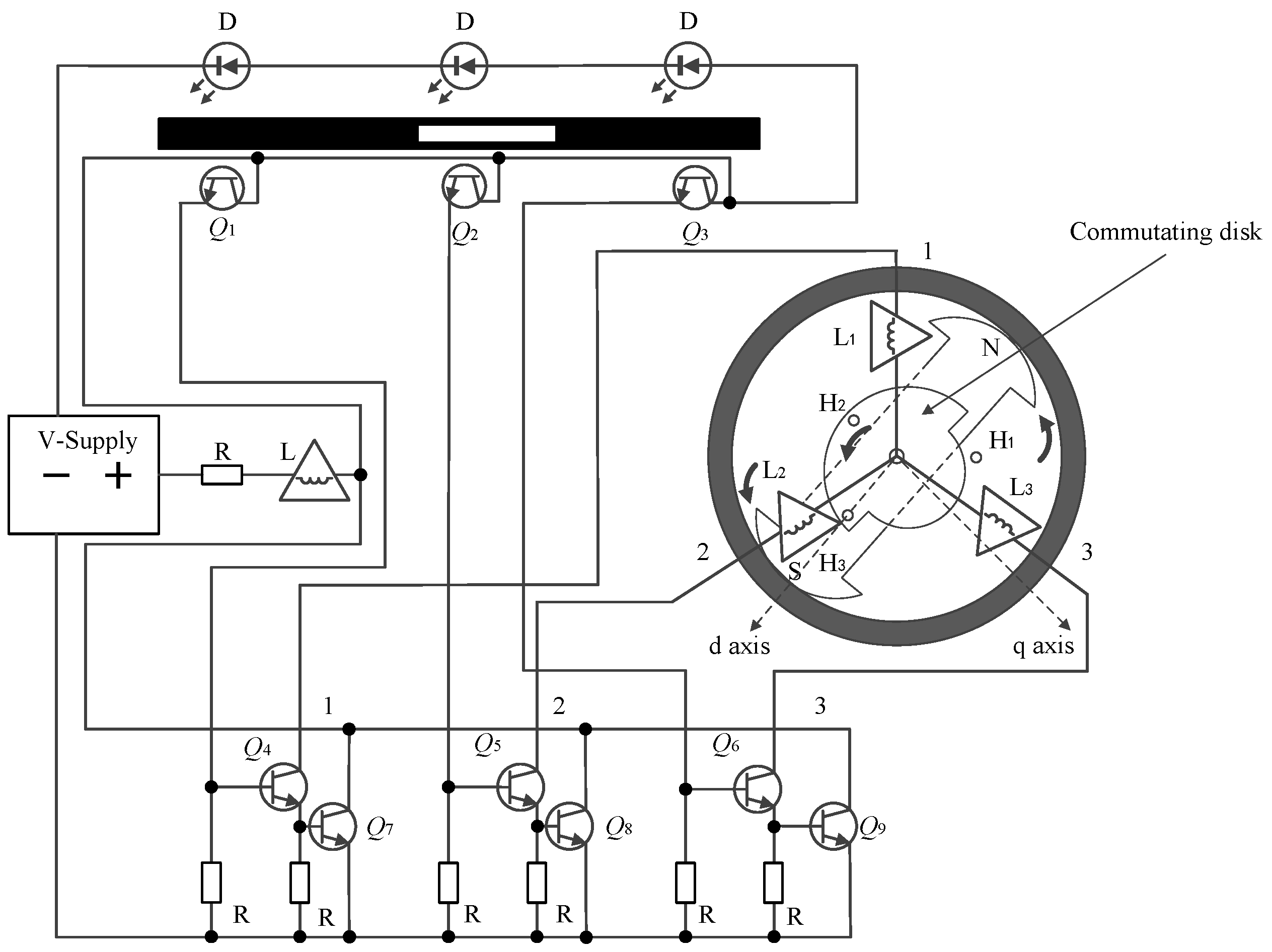
1. Introduction
2. Analytical Solutions
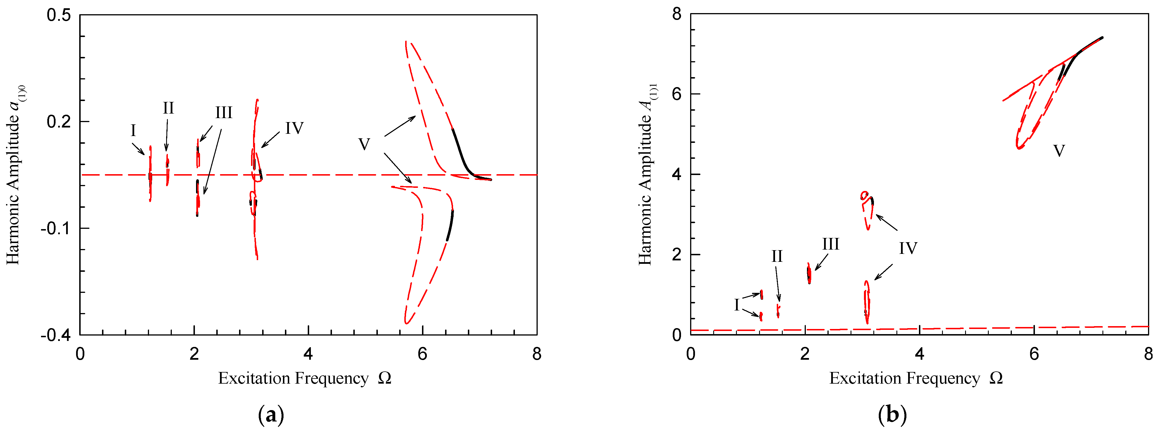
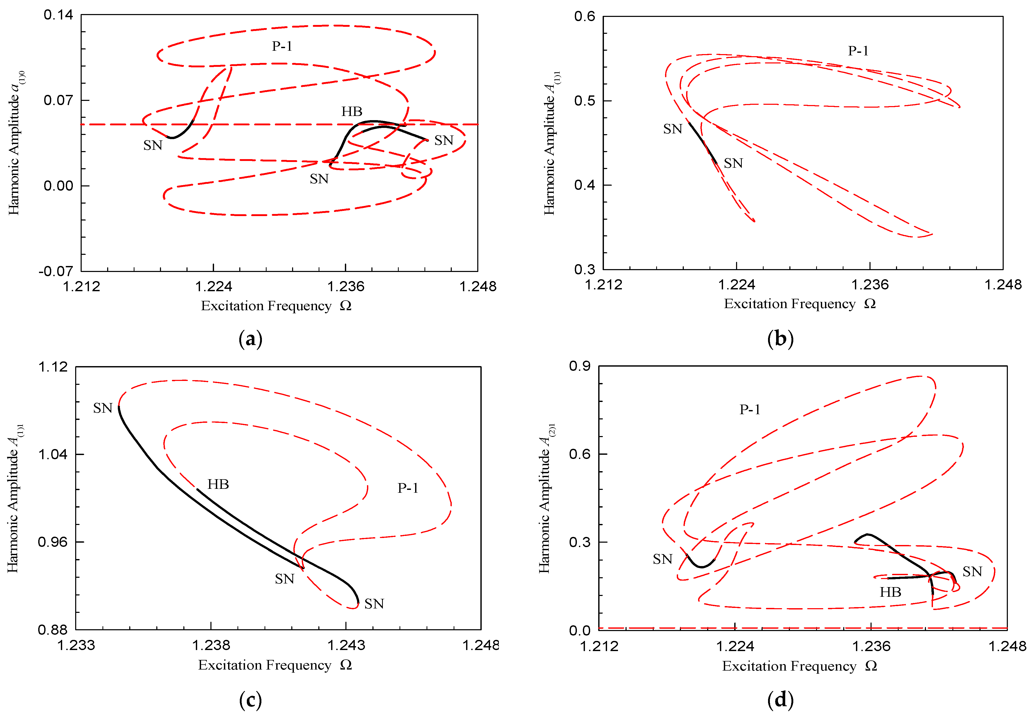
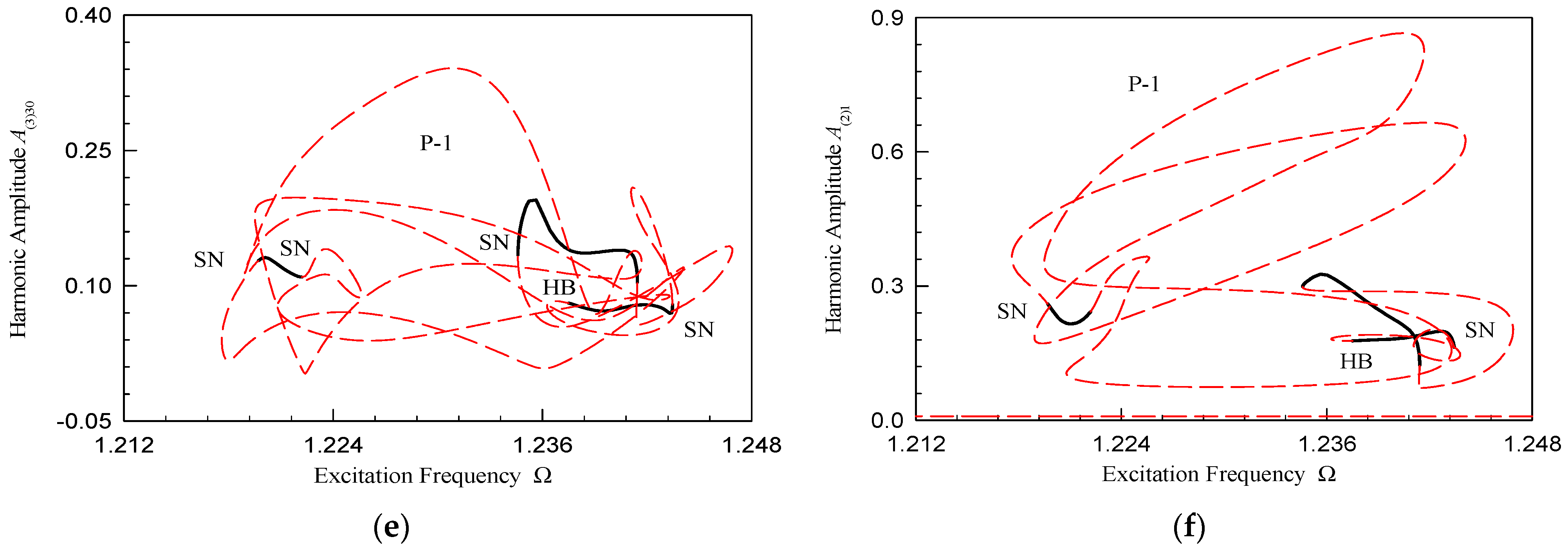
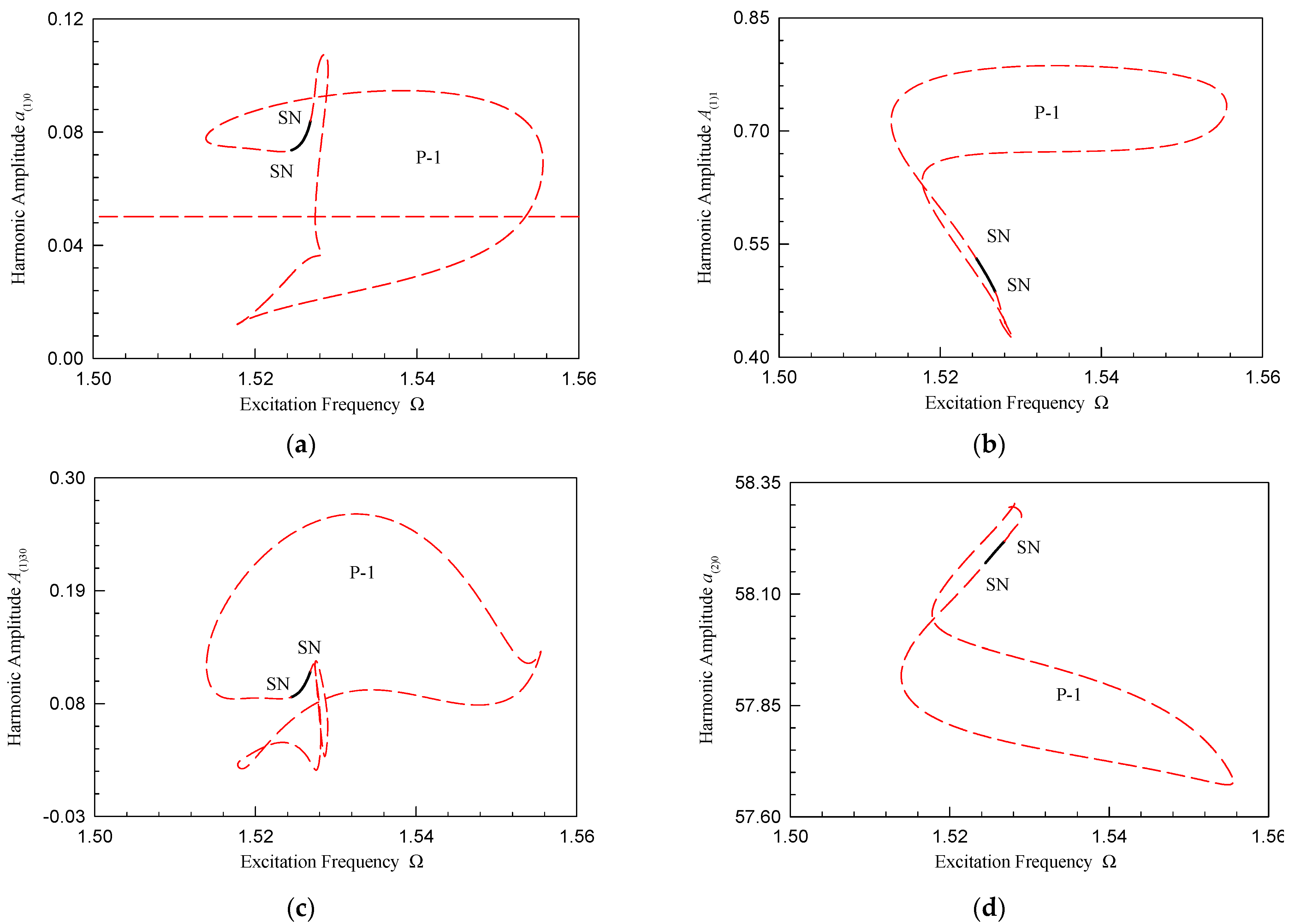
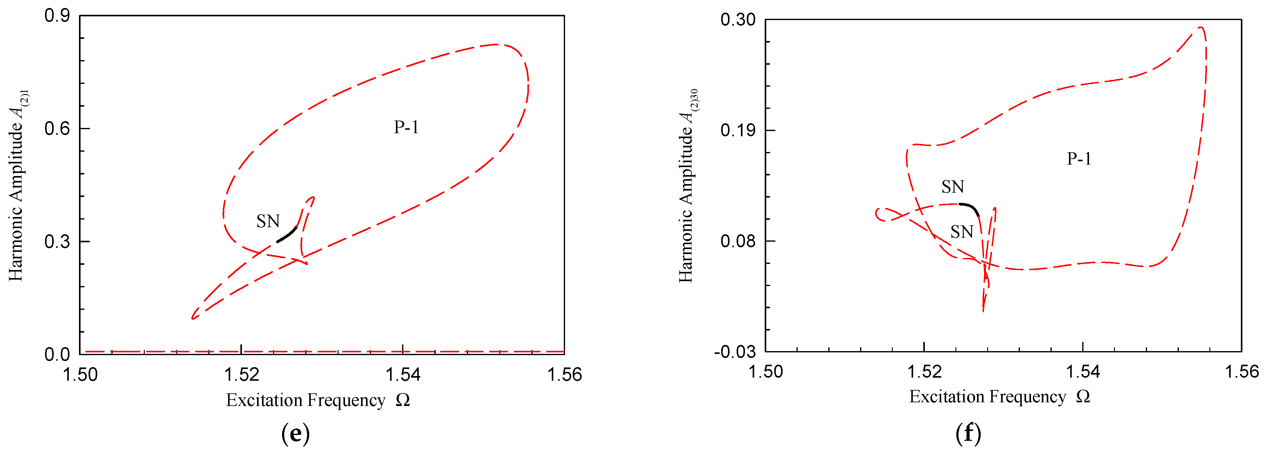
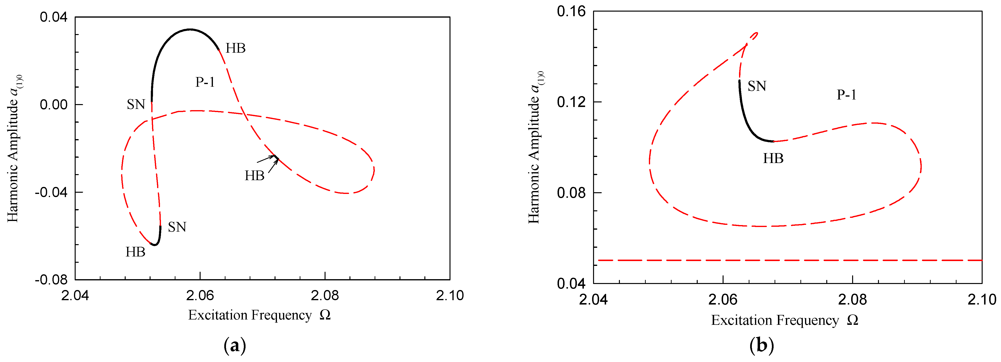
3. Frequency–Amplitude Characteristics
Period-1 Motion
4. Numerical Illustrations
5. Conclusions
Author Contributions
Funding
Institutional Review Board Statement
Informed Consent Statement
Data Availability Statement
Conflicts of Interest
Appendix A
References
- Hemati, N. Dynamic analysis of brushless motors based on compact representations of the equations of motion. In Proceedings of the Conference Record of the 1993 IEEE Industry Applications Conference Twenty-Eighth IAS Annual Meeting, Toronto, ON, Canada, 2–8 October 1993. [Google Scholar]
- Rubaai, A.; Kotaru, R.; Kankam, M.D. A continually online-trained neural network controller for brushless DC motor drives. IEEE Trans. Ind. Appl. 2000, 36, 475–483. [Google Scholar] [CrossRef]
- Prakash, A.; Naveen, C. Combined strategy for tuning sensor-less brushless DC motor using SEPIC converter to reduce torque ripple. ISA Trans. 2023, 133, 328–344. [Google Scholar] [CrossRef] [PubMed]
- Lee, B.-K.; Ehsani, M. Advanced Simulation Model for Brushless DC Motor Drives. Electr. Power Compon. Syst. 2003, 31, 841–868. [Google Scholar] [CrossRef]
- Jabbar, M.; Phyu, H.N.; Liu, Z.; Bi, C. Modeling and numerical simulation of a brushless permanent-magnet dc motor in dynamic conditions by time-stepping technique. IEEE Trans. Ind. Appl. 2004, 40, 763–770. [Google Scholar] [CrossRef]
- Kang, S.-J.; Sul, S.-K. Direct torque control of brushless DC motor with nonideal trapezoidal back EMF. IEEE Trans. Power Electron. 1995, 10, 796–802. [Google Scholar] [CrossRef]
- Kim, I.; Nakazawa, N.; Kim, S.; Park, C.; Yu, C. Compensation of torque ripple in high performance BLDC motor drives. Control Eng. Pract. 2010, 18, 1166–1172. [Google Scholar] [CrossRef]
- Niemczyk, P.; Porchez, T.; Bendtsen, J.D.; Kallesøe, C.S. Hybrid Adaptive Observer for a Brushless DC Motor. IFAC Proc. Vol. 2008, 41, 10213–10218. [Google Scholar] [CrossRef]
- Hemalatha, N.; Venkatesan, S.; Kannan, R.; Kannan, S.; Bhuvanesh, A.; Kamaraja, A. Sensorless speed and position control of permanent magnet BLDC motor using particle swarm optimization and ANFIS. Meas. Sens. 2024, 31, 100960. [Google Scholar] [CrossRef]
- Dasari, M.; Reddy, A.S.; Kumar, M.V. A comparative analysis of converters performance using various control techniques to minimize the torque ripple in BLDC drive system. Sustain. Comput. Inform. Syst. 2022, 33, 100648. [Google Scholar] [CrossRef]
- Li, Z.B.; Lu, W.; Gao, L.F.; Zhang, J.S. Nonlinear state feedback control of chaos system of brushless DC motor. Procedia Comput. Sci. 2021, 183, 636–640. [Google Scholar] [CrossRef]
- Li, C.-L.; Li, W.; Li, F.-D. Chaos induced in Brushless DC Motor via current time-delayed feedback. Optik 2014, 125, 6589–6593. [Google Scholar] [CrossRef]
- Ge, Z.-M.; Chang, C.-M. Chaos synchronization and parameters identification of single time scale brushless DC motors. Chaos Solitons Fractals 2004, 20, 883–903. [Google Scholar] [CrossRef]
- Faradja, P.; Qi, G. Analysis of multistability, hidden chaos and transient chaos in brushless DC motor. Chaos Solitons Fractals 2020, 132, 109606. [Google Scholar] [CrossRef]
- Luo, A.C.; Huang, J. Approximate solutions of periodic motions in nonlinear systems via a generalized harmonic balance. J. Vib. Control 2011, 18, 1661–1674. [Google Scholar] [CrossRef]
- Luo, A.C.J.; Huang, J. Analytical dynamics of period-m flows and chaos in nonlinear systems. Int. J. Bifurc. Chaos 2012, 22, 91–116. [Google Scholar] [CrossRef]
- Luo, A.C.J.; Huang, J. Analytical solutions for asymmetric periodic motions to chaos in a hardening Duffing oscillator. Nonlinear Dyn. 2013, 72, 417–438. [Google Scholar] [CrossRef]
- Luo, A.C.J.; Yu, B. Complex period-1 motions in a periodically forced, quadratic nonlinear oscillator. J. Vib. Control 2015, 21, 896–906. [Google Scholar] [CrossRef]
- Ying, J.; Jiao, Y.; Chen, Z. Further analytic solutions for periodic motions in the Duffing oscillator. Int. J. Dyn. Control. 2016, 5, 947–964. [Google Scholar] [CrossRef]
- Xu, Y.; Luo, A.C.J.; Chen, Z. Analytical solutions of periodic motions in 1-dimensional nonlinear systems. Chaos Solitons Fractals 2017, 97, 1–10. [Google Scholar] [CrossRef]
- Huang, J.; Jing, Z. Feedback control of unstable periodic motion for brushless motor with unsteady external torque. Eur. Phys. J. Spec. Top. 2019, 228, 1809–1822. [Google Scholar] [CrossRef]
- Huang, J.; Xiong, X. Nonlinear behavior for periodically excited brushless motor. COMPEL—Int. J. Comput. Math. Electr. Electron. Eng. 2019, 38, 522–535. [Google Scholar] [CrossRef]
- Gailitis, A.; Brekis, A. Equivalent circuit approach for acoustic MHD generator. Magnetohydrodynamics 2020, 56, 3–13. [Google Scholar] [CrossRef]
- Chen, Z.; Xu, Y.; Ying, J. Analytical Bifurcation Tree of Period-1 to Period-4 Motions in a 3-D Brushless DC Motor With Voltage Disturbance. IEEE Access 2020, 8, 129613–129625. [Google Scholar] [CrossRef]

| P-1 Motion Part | Disturbance Frequency Range |
|---|---|
| I | (1.211, 1.244), (1.235, 1.247) |
| II | (2.0474, 2.0876), (2.0487, 2.0904) |
| III | (5.457, 6.517), (5.698, 7.193) |
| IV | (2.98, 3.083), (3.038, 3.121), (3.004, 3.178) |
| V | (5.457, 6.517), (5.698, 7.193) |
| Figure No. | Ω | Initial Condition | Types |
|---|---|---|---|
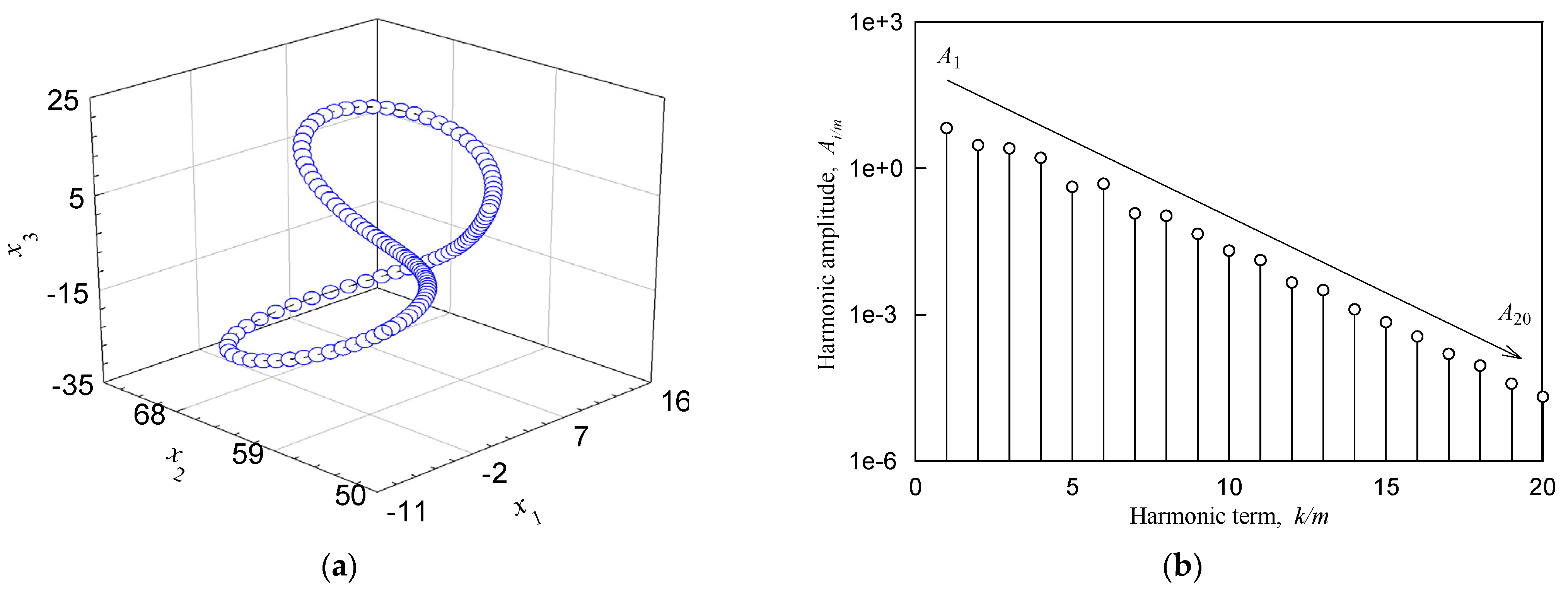
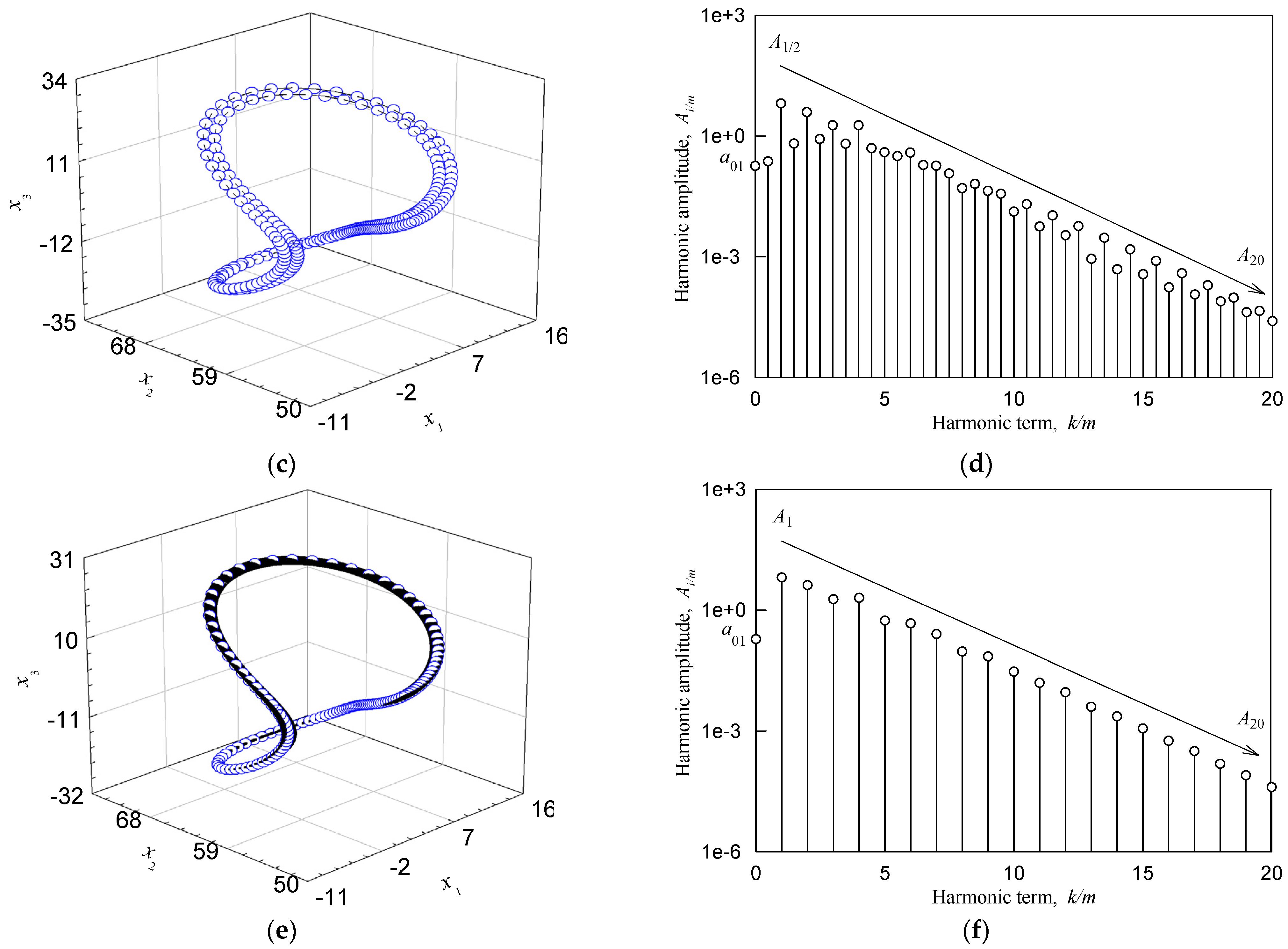
| Figure 6a,b | 6.5 | (5.3227832, 65.525293, 19.302422) | stable P-1 |
| Figure 6c,d | 6.5 | (9.7357535, 55.891501, 13.299756) | stable P-2 |
| Figure 6e,f | 6.5 | (7.5583327, 63.739675, 18.706304) | unstable P-1 |
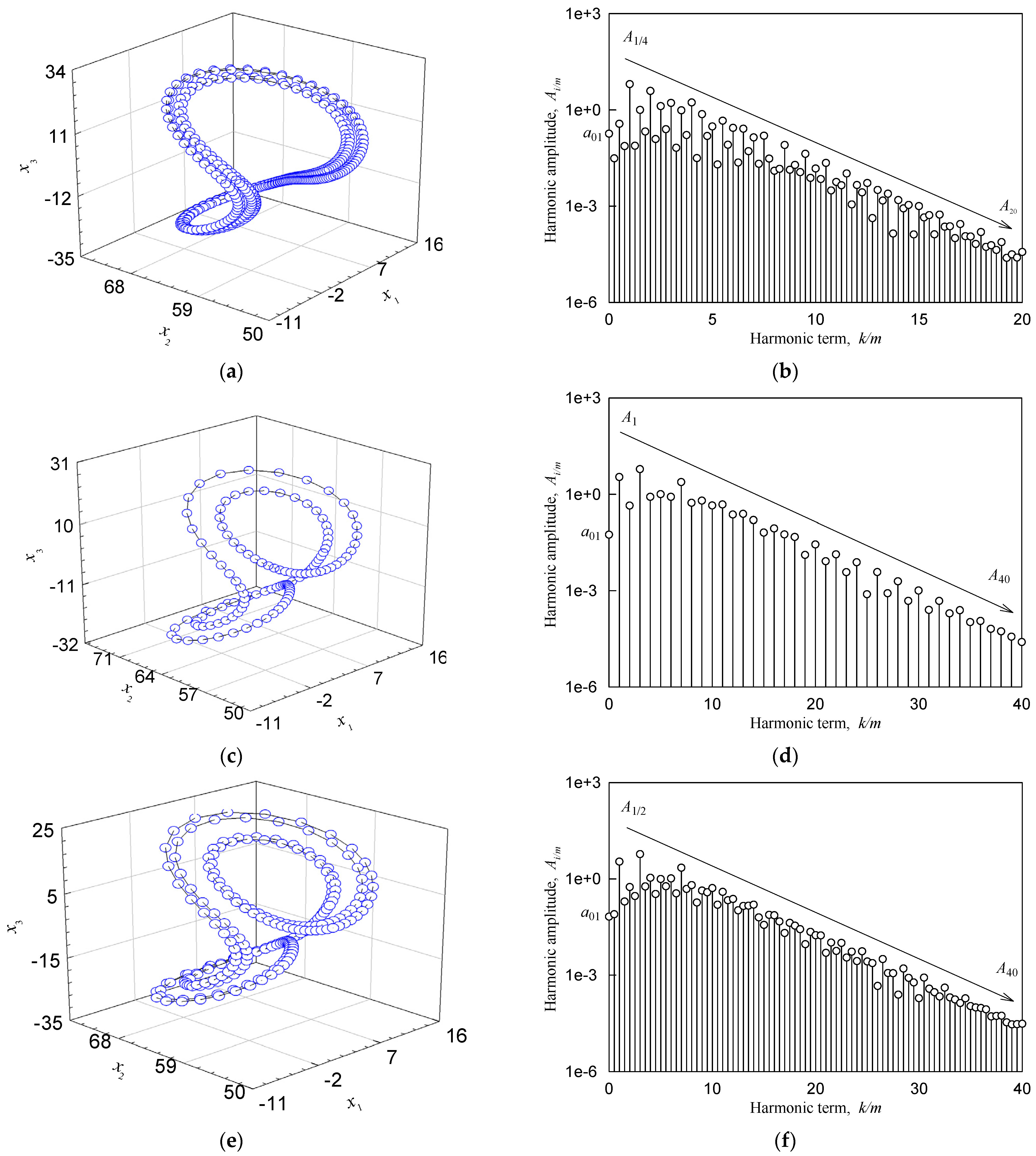
| Figure 7a,b | 6.46 | (10.279434, 58.625938, 15.979369) | stable P-4 |
| Figure 7c,d | 3.16 | (0.8259358, 53.755447, 2.0334629) | stable P-1 |
| Figure 7e,f | 3.14 | (1.2720598, 52.714859, 1.8667075) | stable P-2 |
Disclaimer/Publisher’s Note: The statements, opinions and data contained in all publications are solely those of the individual author(s) and contributor(s) and not of MDPI and/or the editor(s). MDPI and/or the editor(s) disclaim responsibility for any injury to people or property resulting from any ideas, methods, instructions or products referred to in the content. |
© 2024 by the authors. Licensee MDPI, Basel, Switzerland. This article is an open access article distributed under the terms and conditions of the Creative Commons Attribution (CC BY) license (https://creativecommons.org/licenses/by/4.0/).
Share and Cite
Chen, B.; Xu, Y.; Jiao, Y.; Chen, Z. Period-1 Motions and Bifurcations of a 3D Brushless DC Motor System with Voltage Disturbance. Appl. Sci. 2024, 14, 4820. https://doi.org/10.3390/app14114820
Chen B, Xu Y, Jiao Y, Chen Z. Period-1 Motions and Bifurcations of a 3D Brushless DC Motor System with Voltage Disturbance. Applied Sciences. 2024; 14(11):4820. https://doi.org/10.3390/app14114820
Chicago/Turabian StyleChen, Bin, Yeyin Xu, Yinghou Jiao, and Zhaobo Chen. 2024. "Period-1 Motions and Bifurcations of a 3D Brushless DC Motor System with Voltage Disturbance" Applied Sciences 14, no. 11: 4820. https://doi.org/10.3390/app14114820
APA StyleChen, B., Xu, Y., Jiao, Y., & Chen, Z. (2024). Period-1 Motions and Bifurcations of a 3D Brushless DC Motor System with Voltage Disturbance. Applied Sciences, 14(11), 4820. https://doi.org/10.3390/app14114820