Abstract
Active sonar can usually only directly measure the distance and bearing information of underwater targets, and cannot directly obtain target velocity, acceleration and other information. Therefore, the amount of information is relatively small, making it difficult to support the construction of complex motion models. At the same time, the motion state of underwater maneuvering targets is changeable. In response to the problem of detecting and tracking underwater moving targets by active sonar, this paper proposes a target transient model correction (TMC) filtering tracking method. Based on the conventional Kalman filter (KF) estimation, residual covariance is used as a signal quantity. When there is a large change in it, a transient filter with constant gain is adopted to filter the measurement value. The filtered output is used to correct the KF gain matrix and the target motion state model, to avoid the problem of increasing or even diverging KF estimation errors caused by changes in process noise. Using this method can solve the problem of maintaining stability and filtering estimation accuracy of active sonar tracking of underwater maneuvering targets with less computational and engineering costs.
1. Introduction
Active sonar target tracking is based on the discrete point tracks of underwater moving targets detected by sonar. Through track correlation, state estimation and other filtering processing, random errors in the measurement process are suppressed, and the accuracy of target measurements is improved. This makes the target track smoother and allows more state information about the target to be obtained, such as course, speed, acceleration and other parameters. Active sonar target tracking belongs to the category of maneuvering target tracking. For maneuvering target tracking, researchers at home and abroad have mainly conducted a large amount of research work from three directions: maneuvering target motion model, filtering algorithm, and track management. Among them, the motion model and filtering algorithm are the core and key.
In the 1970s, Friedland et al. [1] proposed the constant velocity (CV) model, and Hampton et al. [2] proposed the constant acceleration (CA) model. These two models belong to the most basic linear mathematical models and are mainly suitable for weakly maneuvering targets. In the context of nonlinear motion models, Singer proposed a first-order time-correlated stochastic model with a zero mean of target maneuvering acceleration, known as the Singer model [3], which is suitable for target motion patterns that fall between CV and CA movements. Moose et al. proposed a correlated Gaussian noise model with a random switch mean, known as the semi-Markov model [4,5]. The main difference between the semi-Markov model and the Singer model is that the semi-Markov model introduces non-zero acceleration. In the early 1980s, Zhou proposed the “current” statistical model for maneuvering targets [6,7], which used a more realistic non-zero mean and a modified Rayleigh distribution to characterize the maneuvering acceleration characteristics of targets. To describe the acceleration distribution of maneuvering targets more accurately, Mehrotra et al. extended the derivative of acceleration to a state variable based on the Singer model, and proposed the Jerk model [8,9]. Since the Jerk model adds the derivative of acceleration as a state variable, the description of acceleration is more accurate, which also improves tracking accuracy. The motion form of maneuvering targets is usually complex and variable [10]. When the target’s motion state undergoes significant changes, the preset single model mismatches with the actual motion state, leading to reduced filtering precision, filter divergence, unstable target tracking, and target loss [11]. To address this issue, Blom et al. proposed the interacting multiple model (IMM) algorithm based on generalized pseudo-Bayesian theory [12]. This algorithm has received extensive research and applications in the tracking of maneuvering targets in the air, ground, and water in recent years. The standard IMM algorithm is a recursive algorithm that assumes the motion state of the tracked target can be described by a finite set of models. Multiple models work simultaneously, and the posterior probabilities of each model are used to weight the filtering inputs and outputs. The transition between models is described by a Markov chain process. The IMM algorithm allows the online model to closely approximate the actual motion state of the target and ensures that the inputs of all filters in the system at each discrete sampling time match the actual system state, avoiding filter divergence. These studies can improve the suitability of the model and the real motion of the target, thereby enhancing tracking accuracy.
In terms of tracking filtering algorithms, linear systems often employ two-point extrapolation filtering, Wiener filtering, least squares filtering, α-β [13], α-β-γ [14], and the KF [15] method. For nonlinear systems, the main filtering methods include the classical extended Kalman filtering (EKF) based on nonlinear approximation [16,17], unscented Kalman filtering (UKF) [18], cubature Kalman filtering (CKF) [19], and particle filtering (PF) proposed by Gordon et al. [20]. Many researchers have also optimized and improved these filtering methods. Subsequently, the emergence of improved algorithms such as the error-minimizing squared sum filter, the kernel correlation filter [21], and convolutional neural networks have made significant contributions to more precise target tracking. For specific tracking applications, the choice of filtering algorithm should be based on the availability of prior knowledge about system dynamic noise, sensor measurement error statistics, as well as constraints such as tracking accuracy and computational requirements. A comprehensive trade-off selection should be made.
At the beginning of each scanning period, the active sonar sends a pulse signal and then receives the target echo. By processing and analyzing the echo, the target information is obtained. By measuring and analyzing the time difference between pulse signal transmitting time and echo receiving time, combined with underwater sound propagation speed, the distance value of the target can be obtained directly. By using spatial directivity and multi-beam direction finding processing of the receiving transducer array, the azimuth of the echo can be determined, and the azimuth information of the target can be obtained. When the transmitting pulse signal is a CW signal, if there is relative motion between the target and the sonar, there will be a frequency offset between the transmitted CW signal and the received echo signal. Through spectrum analysis of the echo signal, the radial velocity of the target relative to the sonar can be calculated. Of course, other pulse signals will also have Doppler shifts, but because they are complex wideband signals, extracting accurate Doppler shifts requires more complex algorithms. The “velocity” obtained at this time is only the radial velocity of the target relative to the sonar and not the true speed of the target in the Earth coordinate system. At present, no active sonar can directly measure the acceleration of target motion.
Therefore, the tracking of underwater targets by active sonar has the following characteristics: Firstly, it typically adopts the track while scan (TWS) approach, which involves simultaneously searching, measuring, and tracking target information in a periodic manner. This requires high real-time tracking performance. Secondly, the target measurement information has low dimensionality and a slow update rate. Typically, only azimuth and range information in a two-dimensional plane are available, and direct measurements of target depth, velocity, and other information are generally not possible. Additionally, due to the slow propagation speed of sound waves in water compared to electromagnetic waves, the update rate of measurement information is slow, typically taking tens to hundreds of seconds to obtain the next batch of measurements. Thirdly, the target’s motion state is highly variable and subject to high process noise. Fourthly, the target may easily “lose” due to the influence of the ocean environment and countermeasures, resulting in the inability to acquire target measurement information continuously and stably over multiple scanning cycles. This leads to an increase in tracking output errors, instability, or even filter divergence.
Due to the unique application scenarios, there are relatively few reports in the research of active sonar for tracking underwater maneuvering targets. The Ocean Systems Laboratory in the UK has studied the technology of forward-looking sonar for tracking and localizing underwater targets based on particle filtering [22]; The Florida Atlantic University in the United States has applied the KF algorithm to the forward-looking sonar target tracking processing of remotely operated vehicles (ROVs) [23]. Canada’s El-Hawary has derived a robust EKF algorithm and applied it to underwater moving target tracking [24]. Yang and others have proposed a novel particle filtering algorithm for underwater moving target tracking [25]. References [26,27] proposed a composite filtering method that combines the robustness of particle filtering with the real-time performance of KF, effectively reducing tracking errors. Reference [28] studied the target localization and tracking method based on azimuth Doppler frequency deviation two-dimensional measurement information, which can achieve faster convergence and higher tracking accuracy compared with one-dimensional azimuth measurement information. Liu et al. [29] discussed the application of the CKF algorithm based on the variance square root in torpedo target tracking, aiming at the problem that the covariance can become non-positive definite and cause filter instability or even divergence in high-dimensional systems using the UKF algorithm. Gao et al. [30] studied underwater maneuvering target tracking based on the interactive multiple model (IMM). Zhang et al. [31] addressed the issue that the single--model KF cannot fully adapt to all motion states of underwater targets. They used the interactive multiple model KF method to process the ultra-short baseline tracking data of autonomous underwater vehicles (AUVs). The motion models enhance motion state adaptability through probability matrix transitions. The experimental results demonstrated that this algorithm has better state adaptability than the single--model KF algorithm when the multi-model set is reasonably constructed. Zhao et al. [32] combined EKF and UKF with the IMM algorithm for underwater target tracking. Their research suggests that under high measurement error conditions, the IMM-UKF algorithm has higher tracking accuracy than the IMM-EKF algorithm. In recent years, the algorithm based on depth learning and neural networks has been applied to underwater target tracking to solve model mismatches and other problems and improve tracking stability [33,34,35].
Due to the special nature of underwater target detection, such as submarines, there is a scarcity of statistical characteristics from known target data samples. As a result, solving the probability transition matrix poses one of the significant challenges, given that the Markov chain transition probability in the interactive multiple model tracking method relies on statistical analysis of these data. The selection of the set of maneuvering target motion models is another challenge: if the goal is to cover as many target motion modes as possible, the model set can become very large, and the model space approaches continuity, making the model set countably infinite, leading to a drastic increase in computational complexity and potential model competition, which can even worsen tracking performance. On the other hand, if there are fewer motion models in the model set, it can be difficult to cover all possible target motion modes, leading to insufficient tracking accuracy or even tracking divergence. Therefore, using a multi-model set to describe the motion of the target can, to some extent, overcome the limitations of the single model. However, the computational complexity of the multi-model approach is high, requiring a high level of prior information about the target, which leads to an increase in computational resources. This may not be suitable for some engineering applications. Additionally, when active sonar is used to detect underwater submarines that maneuver evasively, changes in target reflectivity and dynamics can cause periodic measurement values to be lost (i.e., periodic measurement information is not continuous), lead to a decrease in tracking performance and even loss of target tracking.
To address the problem of active sonar tracking of underwater submarine targets, this study proposes a novel underwater maneuvering target tracking method based on transient correction using random mixing models. This approach assumes that, although the motion state of maneuvering targets is complex and varies over time, within a certain time period, underwater targets only have one maneuvering mode that can be described by only one motion model. Therefore, the focus of this approach is how to determine whether the target’s maneuvering mode has changed, and once such a change occurs, how to correct and adjust the motion model parameters to make the corrected motion model closer to the true motion state of the target.
2. Description of the TMC Tracking Method
Based on the following two points of analysis, the overall design approach of the algorithm and the overall schematic diagram as shown in Figure 1 are presented:
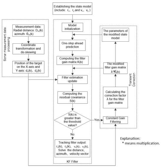
Figure 1.
Schematic diagram of the general idea of the TMC tracking method.
- Due to the characteristics of submarine targets and water media, when a submarine target is moving underwater, sudden changes in maneuvering state generally do not occur. In combination with the long measurement acquisition period of active sonar for underwater submarine targets, it can be assumed that within two sampling intervals, the change in target motion state is uniform, and the motion state changes that occur within a number of consecutive sampling periods can be considered a transient process. By correcting this transient process, the tracking instability or decreased accuracy caused by changes in motion mode can be solved.
- In general, after given design requirements, the precision of active sonar target measurement data is stable. Therefore, the deviation between target measurement values and state estimation values can be considered to be caused by changes in their motion state. According to the changes in the variance of measurement values or state estimation values, it can be judged whether the target’s motion state has changed, and the motion state parameters can be corrected to make the motion model closer to the true motion state of the target.
As shown in Figure 1, the system state model is first established, including the displacements (rx, ry) and velocity components (vx, vy) on the X-axis and Y-axis. Then, the state model is initialized and assigned values. Subsequently, KF processing is performed according to the flow of one-step advance prediction, filtering gain matrix calculation, and filtering estimation update. Additionally, the residual covariance of the current cycle is calculated and analyzed. When is less than the preset decision threshold, the KF result is used as the tracking filter output. When it is greater than the preset decision threshold, it is judged that there is a significant deviation between the current state model and the actual motion of the target, and thus correction is necessary. Using the constant gain filtering method, the current measurement value is filtered, and the KF gain matrix is adjusted based on the filtering result. Additionally, the motion velocity, position, and process noise of the state model are corrected. With the corrected state model parameters and filter gain matrix, the KF process is re-performed. Under normal circumstances, the active sonar receives the echo signals reflected by the target and processes the echo signals to obtain direct measurement information such as radial distance and azimuth information. For the KF algorithm that models and processes tracking in a Cartesian coordinate system, it is necessary to perform coordinate system transformation and deflection removal processing on the measurement data to obtain the displacement information (, ) of the target on the X-axis and Y-axis in the Cartesian coordinate system, which is used as the measurement update for tracking filtering.
2.1. System Model
In general, within a single measurement period of active sonar, only the radial distance and azimuth of underwater targets can be obtained. With sonar as the observation origin O, a two-dimensional coordinate system is establish ed, as shown in Figure 2 (for convenience of expression, let the Y-axis point to the north). The following Equations (1) and (2) are proposed to describe the target motion model shown in Figure 2: at time t, the target is located at Pt point, with a distance of and an azimuth of ; at time (T is the observation period of active sonar), the target is located at Pt+T point with a distance of and an azimuth of . The displacement of the target on the X-axis and Y-axis from time t to time is:
in which and are the projections of the radial distance of the target at time t on the X- and Y-axis, respectively, and are the projections of the radial distance of the target at time on the X- and Y-axis, respectively.
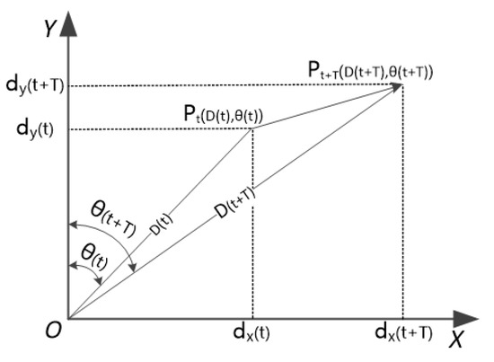
Figure 2.
Schematic diagram of target movement situation.
2.1.1. State Equation
When a slowly varying target like a submarine is moving underwater, most of the time, the speed changes are weak. Therefore, it can be assumed that most of the time, it is in a uniform motion state, and the acceleration can be regarded as a random disturbance with Gaussian white noise characteristics, usually with a zero mean and a variance of . Therefore, the continuous-time state equation of the target can be established as:
In the formula, represents the system state vector, and . and represent the target’s displacement on the X- and Y-axis, respectively, while and represent the target’s velocity on the X- and Y-axis, respectively. and represent the accelerations expressed in terms of random noise , with mean and variance given by:
is the state transition matrix.
is the process noise input matrix: .
The discrete-time state equation for a constant system is:
In the formula, represents the discrete state vector, and , and represent the target’s displacement on the X- and Y-axis, respectively, while and represent the target’s velocity on the X- and Y-axis, respectively. The state transition matrix is defined as:
The process noise input matrix is:
The process noise matrix is defined as:
The covariance matrix of the process noise is defined as:
2.1.2. Measurement Equation
In the rectangular coordinate system, the measurement equation is:
In the formula, represents the measurement vector, where . is the measurement matrix:
is the measurement noise matrix, and the measurement noise is Gaussian white noise with a mean of zero, variance of , and a normal distribution. Its covariance matrix is defined as:
2.1.3. Measurement Debiasing
In the system model described in Figure 2, when the sonar acquires the radial distance and azimuth measurement values of underwater targets, and , the measurement vector needs to be solved according to Formula (1). Due to the nonlinear transformation included in Formula (1), the measured vector in the Cartesian coordinate system is biased, and it needs to be debiased through compensation.
It is assumed that the measurement errors of the radial distance and azimuth are uncorrelated and follow a zero-mean Gaussian distribution, with variances of and , respectively. The projected targets’ radial distances and on the X- and Y-axis after debiasing compensation are:
In the formula, the value of is:
The noise covariance matrix of the compensated position measurement is:
in which:
in which:
2.2. Tracking Filtering Method
When the target is moving at a constant velocity, the KF algorithm is equivalent to the filtering method designed using the minimum mean squared error estimation criterion in steady state. However, during the transient process or when the target undergoes random maneuvering, the performance of KF is superior to other methods. Additionally, KF is a recursive algorithm that only requires the current time’s prediction and measurement values to obtain the current time’s state filtering estimate, without the need to transmit all historical data. Therefore, it has advantages such as small computational complexity, strong real-time performance, and easy engineering implementation. Based on the above considerations, KF is adopted as the tracking filtering method.
In target tracking, the KF algorithm mainly implements the functions of prediction and filtering estimation. The filtering equation is:
In the formula, represents the filtered estimate at time ; is the priori filtered estimate (one-step advance prediction) of obtained by the measurement value at time :
represents the filtering gain matrix:
is the covariance matrix of one-step advance prediction error:
is the covariance matrix of filtered estimation error:
is the residual (innovation) vector:
is the predicted measurement value:
The covariance matrix of the residual vector is:
The system state vector contains the displacement and motion velocity of the target on the X- and Y-axis. Through the filter processing of Equation (20), the displacement and motion velocity of the target on the X- and Y-axis are constantly updated. After filtering, the distance and azimuth accuracy of the target is improved. The velocity component of the target movement is synthesized by the velocity component of the two directions. Further, if the measurement vector includes the speed measurement of the target, you can establish the state vector that contains the acceleration (the acceleration is no longer considered a random interference noise), and after filtering, you can obtain the motion acceleration components on the X- and Y-axis, and you can obtain the acceleration vector on the two-dimensional plane by the synthesis of the two acceleration components.
2.3. Transient Correction
When the system state equation deviates from the actual situation, the system uncertainty increases, the estimation error of the KF filter becomes larger, and the reliability of the one-step prediction estimation decreases. At this time, KF adjusts the estimation by changing the filtering gain to ensure that the filtered estimation is as close as possible to the actual state . When the motion state of the underwater target changes, it causes an increase in the system process noise described in Section 3.1.1. As a result, the covariance matrix of the one-step advance prediction error becomes larger, and subsequently, the filtering gain also increases. Considering an extreme case where approaches infinity, we take the limit of Equation (22) as follows:
By combining Formulas (25), (26) and (28), we can rewrite Formula (20) as . This indicates that when the system error reaches its limit, the KF system adjusts the reliability of the one-step prediction estimate to the lowest level, while the weight of the measurement variables reaches its maximum.
Therefore, the residual covariance of the variable gain KF filter can be used as a signal indicator, and the residuals of the constant gain filter can be used as a reference to correct the KF filter gain matrix and reset the state model. This process can be iterated.
The comparison judgment threshold of the residual covariance in Figure 1 can be obtained through error analysis of the target measurement history data of the sonar system. Normally, after the design of the sonar is completed, its measurement error is known. Therefore, the comparison threshold for can be determined beforehand.
The constant gain filter selects the αhe filtering method. The αil filter is a constant residual filter that has good convergence properties and can rapidly track maneuvering targets over a wide range. The α-β filtering equation is as follows:
In the equation, and represent the current and previous moment’s target position filtered estimation values, respectively. and are the filtering coefficients, while and represent the current and previous moment’s target velocity filtered estimation values, respectively. is the current moment’s target position measurement value, and is the measurement update period. The αs filter gain is a constant , and the residual is defined as:
When the residual covariance of the KF exceeds the comparison judgment threshold, we select the N residual values before time k to perform mean processing on . The result is then divided by the residual of the α-β filter to obtain the correction factor for the KF filter gain matrix:
3. Simulation Verification and Offshore Testing
In order to verify the effectiveness of the above method, we simulate the underwater trajectory of the submarine target and the measurement information (azimuth and distance) of the submarine target during each scanning period of the active sonar. At the same time, we also carried out a sea test of sonar detection and tracking of submarine targets to further verify the feasibility of the TMC method.
3.1. Simulation Verification
The conventional KF tracking processing and the proposed TMC tracking processing are applied to the simulation data, and the tracking output results are compared.
3.1.1. Simulation Conditions
The underwater target trajectory is composed of five segments, and the motion parameters for each segment are shown in Table 1 [36]. The initial speed of the target is 2.06 m/s, the heading is 90°, and the total duration of motion is 1140 s. At the end of the trajectory, the target speed is 13.35 m/s, and the heading is 47.6°.

Table 1.
Simulation parameters for underwater target motion.
Assuming an active sonar detection scan period of 20 s, the root mean square error (RMSE) of the target’s radial distance measurement is 100 m, and the RMSE of the azimuth measurement is 0.5°. The true trajectory of the target’s motion and the sonar measurements are shown in Figure 3. Specifically, in Figure 3a, when converting the target’s radial distance and azimuth measurements into X- and Y-axis distance measurements in a Cartesian coordinate system, the debiasing process described in Section 2.1.3 was applied.
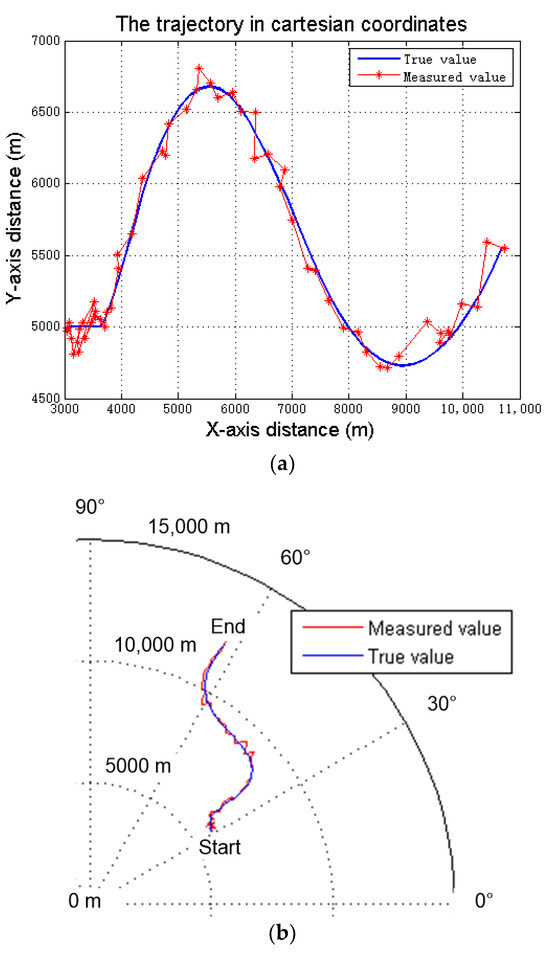
Figure 3.
True trajectory and sonar measured values of the underwater simulated target. (a) The trajectory in cartesian coordinates, (b) The trajectory in polar coordinates.
3.1.2. Simulation Results and Analysis
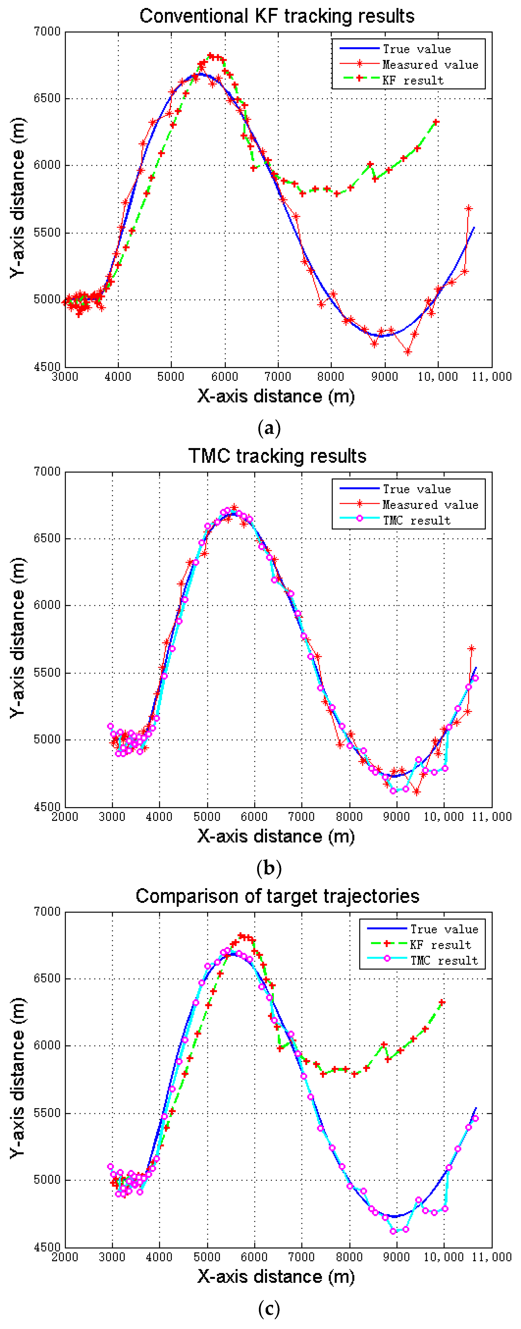
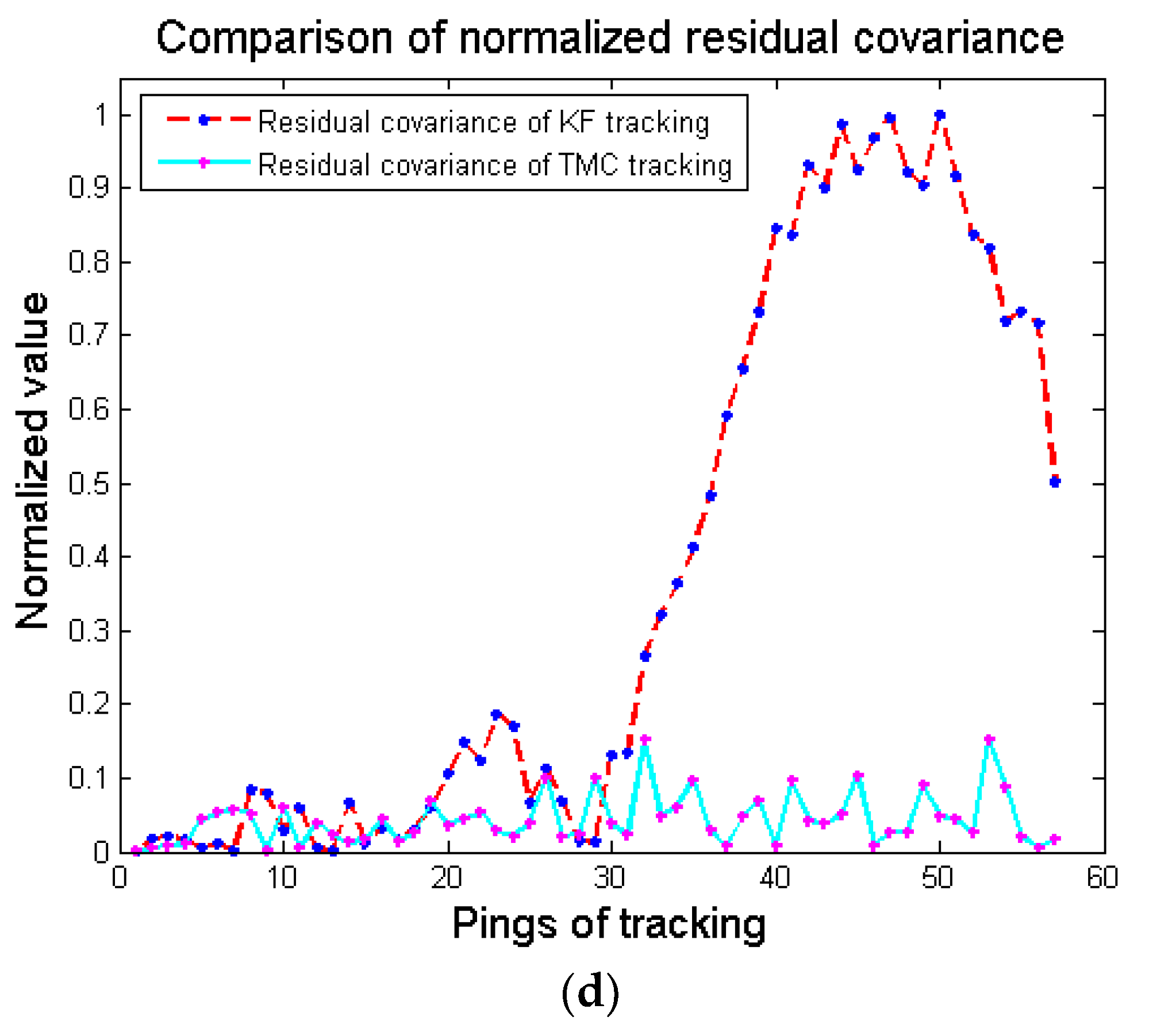
Figure 4 compares the processing results of the simulation data using the conventional KF tracking method and the TMC tracking method. In Figure 4a, when the target transitions from uniform to accelerated motion, the tracking trajectory starts to deviate from the true target trajectory, and the tracking error gradually increases. In Figure 4b, when using the TMC tracking method, the target tracking trajectory deviates less from the true trajectory. Figure 4c further compares the tracking results of the conventional KF method with those of the TMC method. It is evident that the tracking performance of the TMC method is superior to that of the conventional KF method. In Figure 4d, the residual covariance of the two tracking methods is compared after normalization. During the first 15 scan cycles (when the target is in uniform motion), the residual covariance of the KF tracking is relatively small. As the target transitions into accelerated motion after three cycles (after the 18th scan cycle), the residual covariance of the KF tracking gradually increases. The residual covariance of the TMC tracking method is comparable to that of the KF tracking during the uniform motion stage and the initial period of accelerated motion. In the latter half of the trajectory, as the residual covariance of the KF tracking gradually increases, the residual covariance of the TMC tracking method remains at a relatively low level comparable to that during the uniform motion stage.

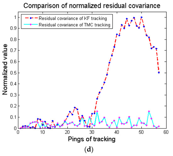
Figure 4.
Comparisons of tracking results between the conventional KF method and the TMC method. (a) Conventional KF tracking results, (b) TMC tracking results, (c) Comparison of target trajectories, (d) Comparison of normalized residual covariance.
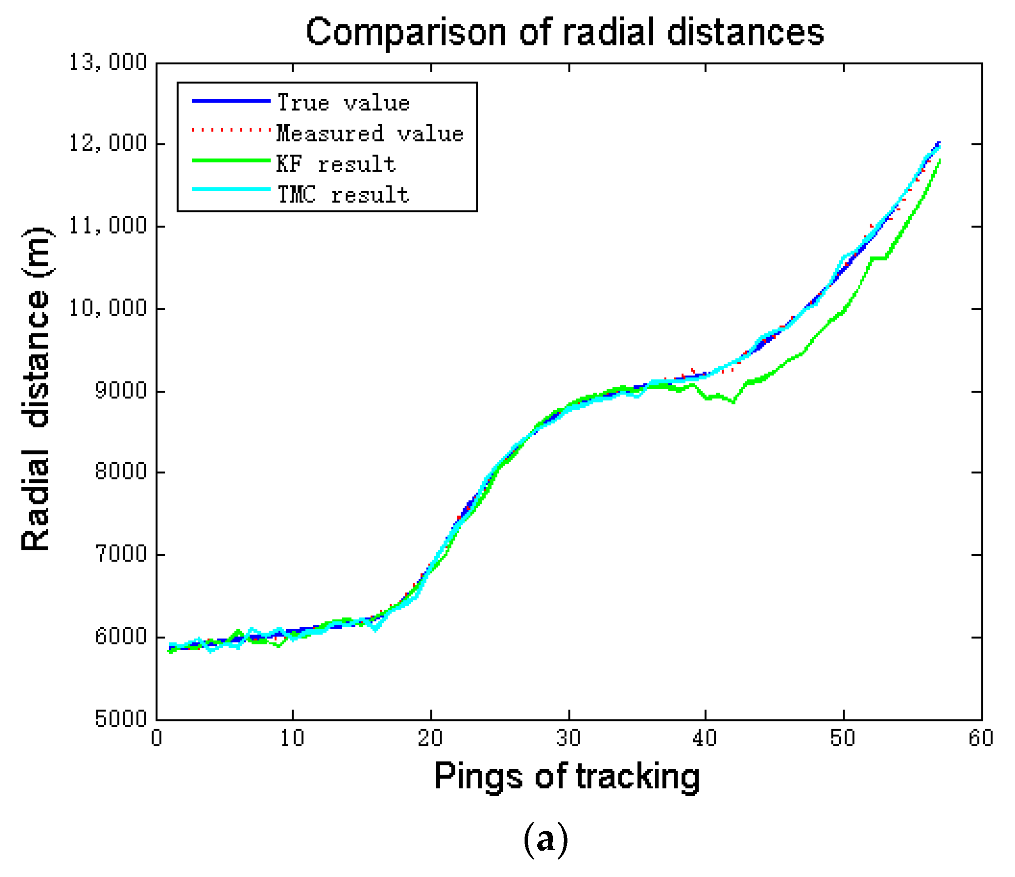
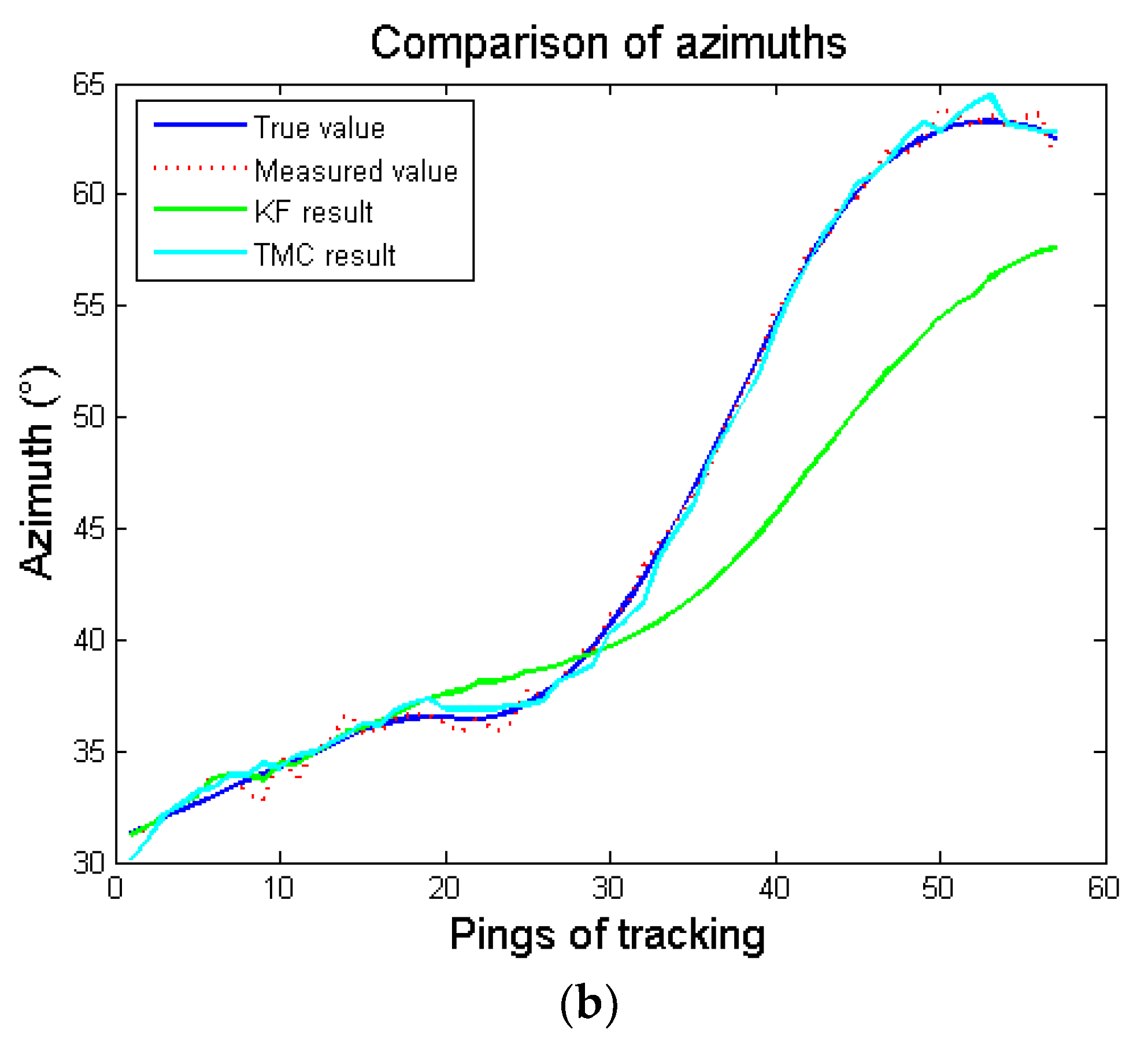
The target’s distances on the X- and Y-axis obtained from both KF tracking and TMC tracking are converted to the target’s radial distance and azimuth for comparison with the true value and measurement value, as shown in Figure 5. To illustrate the deviation of the measurement or tracking estimation points from the true target position, the position distance error is defined as the straight-line distance between the true target position and either the measurement point position or the filtered output position of the target tracking. The RMSE of the position distance and azimuth for KF tracking are 237.5 m and 5.17°, respectively, while those for TMC tracking are 57.33 m and 0.49°, respectively. The TMC tracking method improves the accuracy of both the target’s radial distance and azimuth tracking.

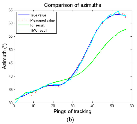
Figure 5.
Comparisons of radial distances and azimuths. (a) Comparison of radial distances, (b) Comparison of azimuths.
Mean-square error (MSE) analysis of the simulation test results was carried out, as can be seen in Table 2. Due to model mismatch, the KF tracking MSE significantly increased. However, after the TMC method is processed, the tracking error can be reduced.
Table 2.
MSE of simulation test.
3.2. Offshore Testing
The experimental site is located in the South China Sea and uses active hull sonar mounted on surface ships to search for and track real underwater submarine targets.
3.2.1. Offshore Testing Description
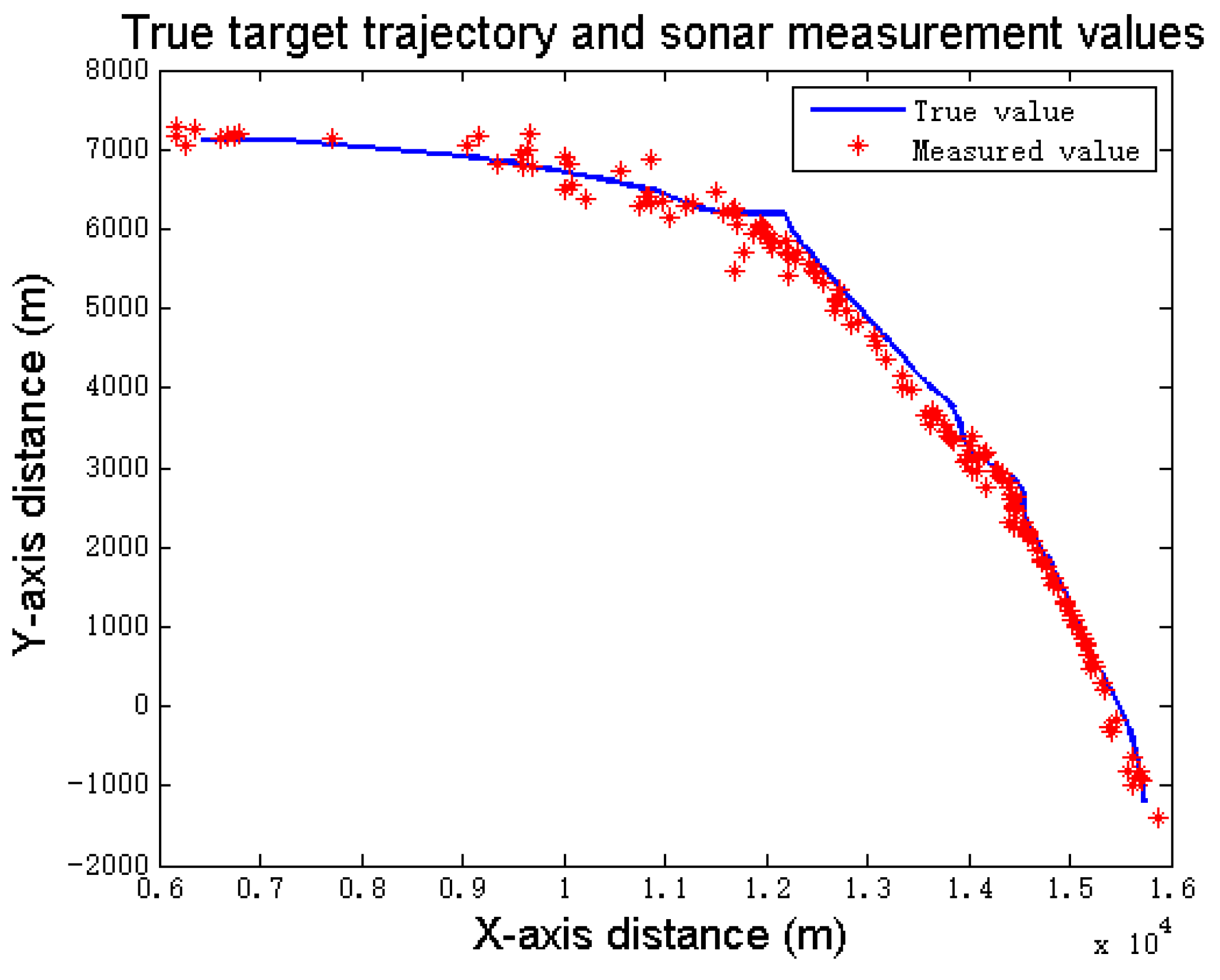
The tracking duration is approximately 4114 s, with a sonar scan period of approximately 17.1 s, resulting in a total of approximately 240 scan cycles. Due to changes in the relative motion of the target and the sonar, resulting in fluctuations in the amplitude of the echo signal, as well as target shift, steering maneuver, etc the measurement data are not continuously sampled. In practice, a total of 155 cycles of underwater target radial distance and azimuth measurements were collected. Figure 6 shows the true target track derived from the underwater target navigation equipment data, as well as the position measurements obtained by converting the target’s radial distance and azimuth detected by active sonar into Cartesian coordinates.
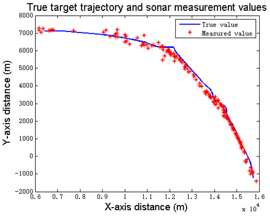
Figure 6.
True target trajectory and sonar measurement values.
3.2.2. Results and Analysis
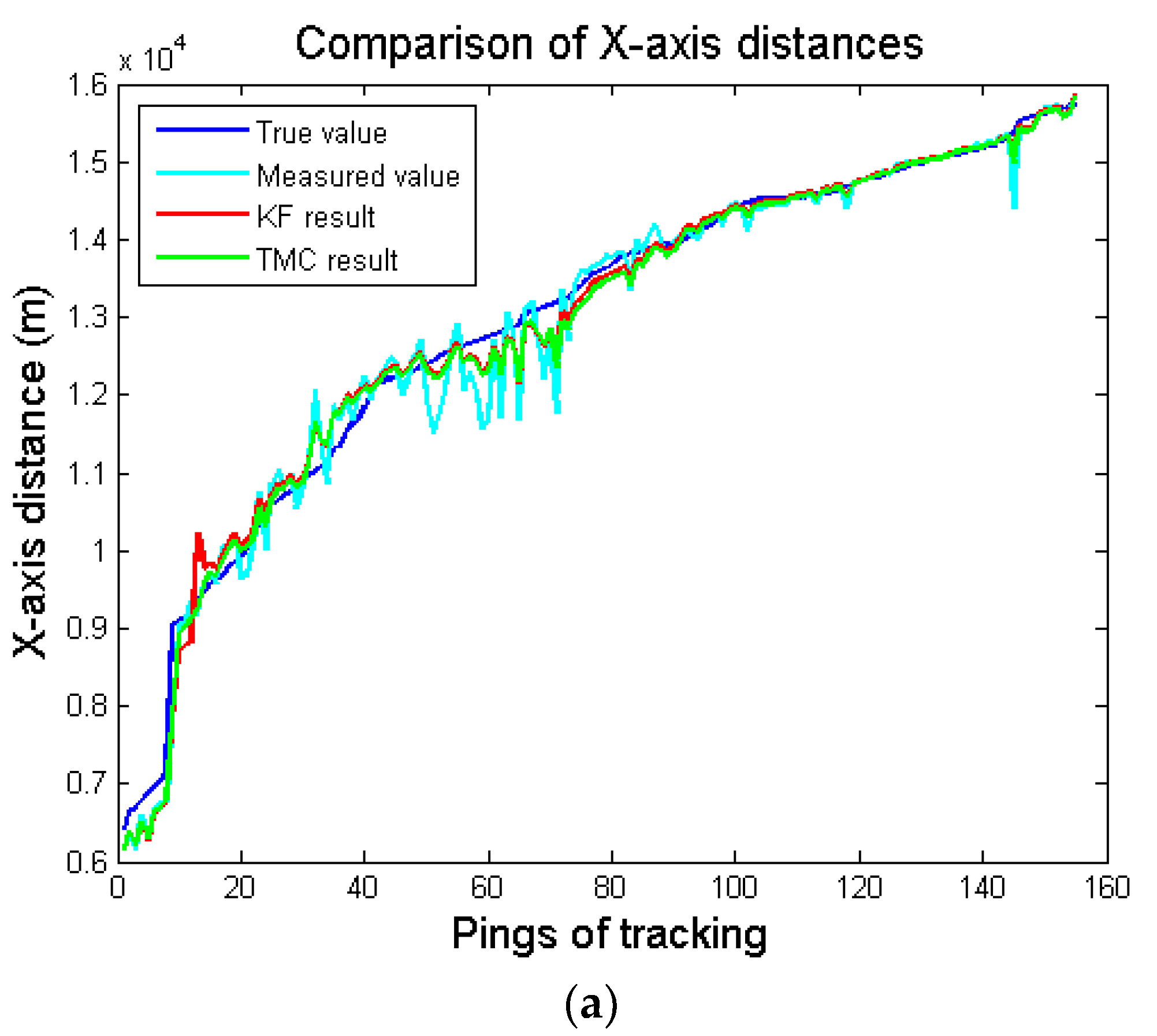
Assuming an RMSE of 100 m for the target’s radial distance measurements and an RMSE of 1.0° for the azimuth measurements, both the conventional KF tracking method and the TMC tracking method were used to track the underwater target. A comparative analysis was conducted on the target’s X-axis distance, Y-axis distance, radial distance, and azimuth obtained from the true values, measurements, KF tracking results, and TMC tracking results. The results are shown in Figure 7.
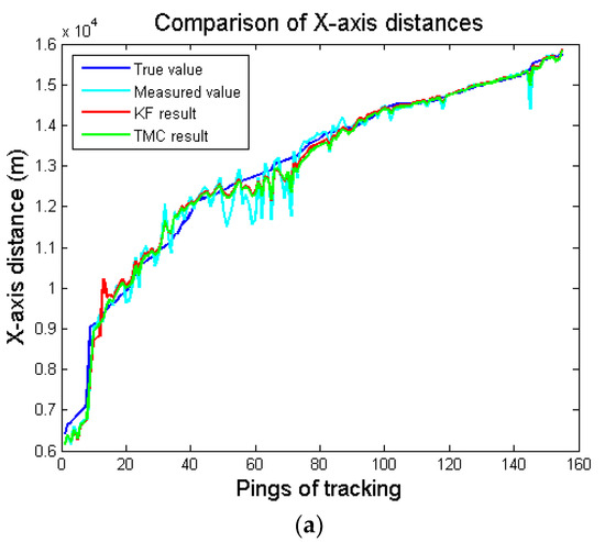
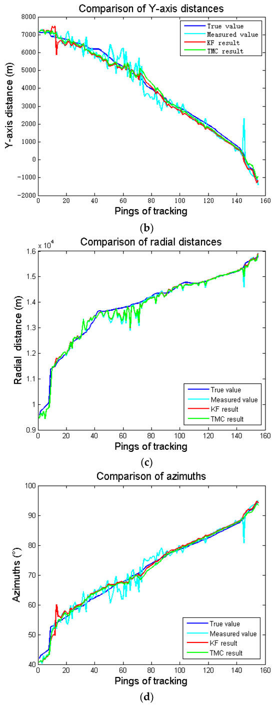
Figure 7.
Comparison of Target’s X-axis, Y-axis, Radial Distances, and Azimuths. (a) Comparison of X-axis distances, (b) Comparison of Y-axis distances, (c) Comparison of radial distances, (d) Comparison of azimuths.
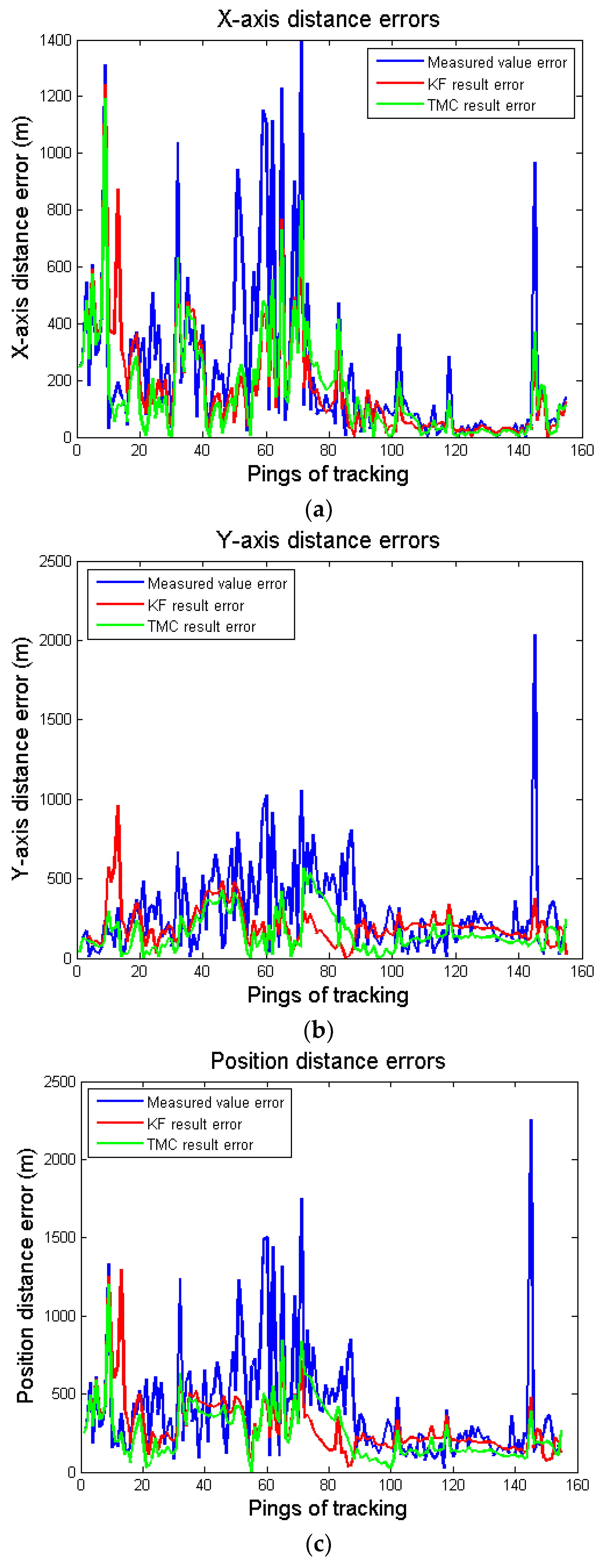
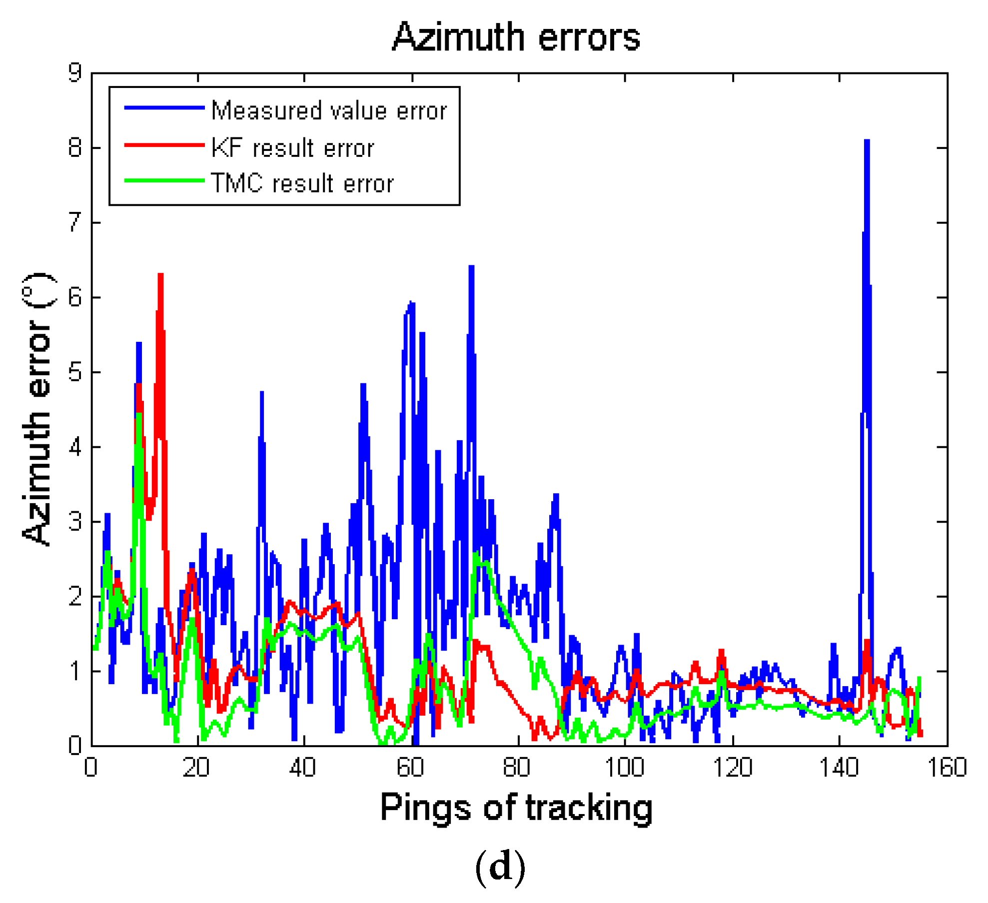
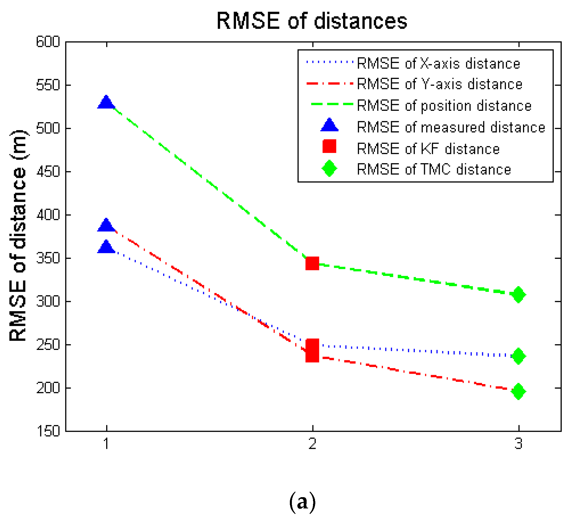
Furthermore, using the true target position as a reference, the absolute errors between the measurement values, KF tracking results, and TMC tracking results and the true values were calculated. The results are shown in Figure 8. The root mean square values of the errors were then calculated and are presented in Table 2 and Figure 9.
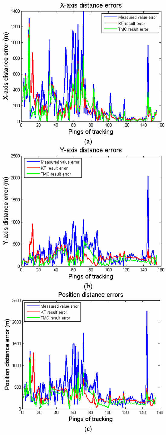

Figure 8.
Comparisons of distance and azimuth errors. (a) X-axis distance errors, (b) Y-axis distance errors, (c) Position distance errors, (d) Azimuth errors.
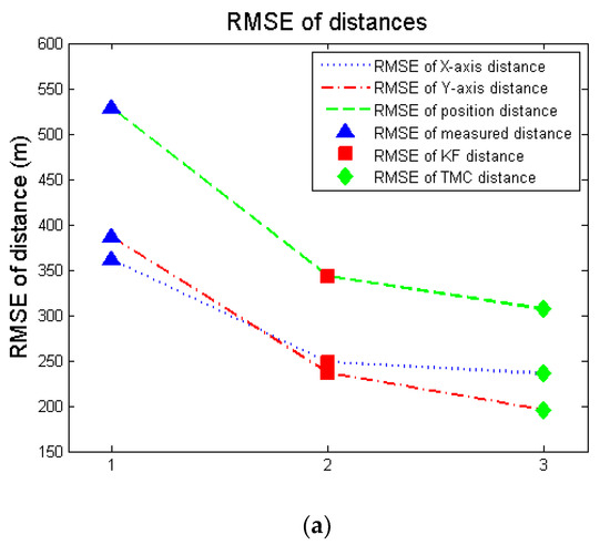
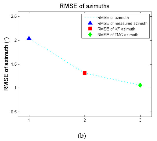
Figure 9.
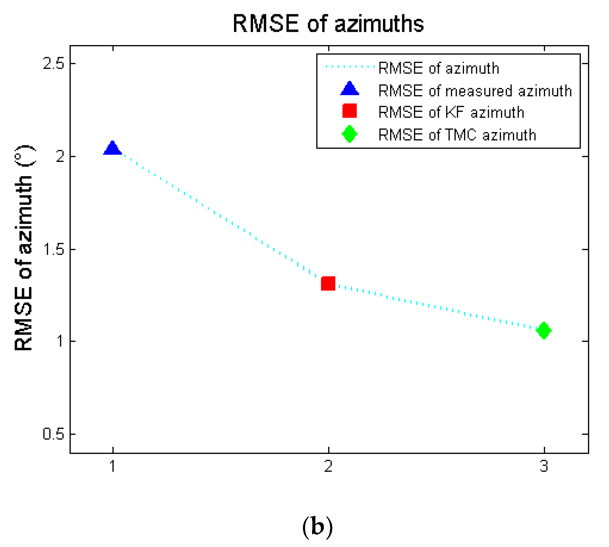
RMSE of distances and azimuths. (a) RMSE of position distances, (b) RMSE of azimuths.
As can be seen from Table 3, after using KF tracking processing, the RMSE of the target’s position distance and azimuth were reduced by 186.07 m and 0.73°, respectively, compared with the RMSE of the sonar measurements. Furthermore, when the TMC tracking method was applied, the RMSE of the target’s position distance and azimuth were further reduced: compared with the KF tracking method, the RMSE of the target’s position distance was reduced by 36.08 m, and the RMSE of the azimuth was reduced by 0.25°.
Table 3.
RMSE of offshore testing.
MSE analysis of the offshore testing results was carried out, and as can be seen from Table 4, the TMC tracking method reduced tracking error, and performance was due to the KF tracking method.
Table 4.
MSE of offshore testing.
Through analysis of the offshore testing data, it can be seen that the TMC tracking method can modify the target motion state equation in real time, so as to make it as close to the real target motion state as possible, rather than tracking according to the established target motion state equation as the KF method. Therefore, the TMC method can improve target tracking accuracy. When analyzing the offshore test data, if the measurement error of sonar on underwater target changes greatly, the performance of the TMC method may be affected. This is because, in a test, if the measurement error of sonar on an underwater target position changes greatly due to various factors (obviously beyond the normal measurement error range of sonar), the TMC method cannot accurately determine whether this change is caused by a change in the submarine target motion state or an increase in measurement error.
4. Conclusions
In order to solve problems such as state model mismatch and tracking accuracy decline caused by changes underwater target motion states, this study investigated and proposeed the TMC tracking method, which innovatively adopts the idea of real-time model correction. Firstly, a KF filter is applied to track the target detected by sonar. The proportion of newly entered measurement information in the forecast output will be smaller and smaller, so that the KF filter cannot keep up with the change in the target state in time. At this time, by comparing the residual covariance of the KF filter with the threshold generated by sonar measurement error, the change in the target motion state can be judged in real time. Then, a constant gain filter is used to modify the target motion model so that it is closer to the real motion state of the target so as to achieve the purpose of transient correction of the KF filter and to improve the precision of the target tracking output. Simulation verification and offshore testing showed that the TMC tracking method could improve the tracking accuracy of active sonar on underwater targets compared with the conventional KF method.
In this research, it was found that variation in the position measurement error of an active sonar on an underwater target will affect the performance of the TMC tracking method. In addition, based on the fact that active sonar can only measure the radial distance and azimuth of a target in real time, this study only established a two-dimensional motion model of a target. If active sonar can measure the target information of more dimensions in real time, such as velocity information, then the algorithm model can be extended to a higher dimension, the corresponding constant gain filter used for transient model correction will also adopt a higher dimension filter (such as α-β-γ filter, etc.), and the algorithm processing effect will be better. Both are worth continuing.
Author Contributions
Conceptualization, C.L. and S.F.; methodology, S.F. and C.L.; software, C.L.; validation, C.L. and S.F.; formal analysis, C.L.; investigation, C.L. and S.F.; resources, S.F.; data curation, C.L. and S.F.; writing—original draft preparation, C.L; writing—review and editing, C.L. and S.F.; visualization, C.L.; supervision, S.F.; project administration, S.F.; funding acquisition, S.F. All authors have read and agreed to the published version of the manuscript.
Funding
This research received no external funding.
Institutional Review Board Statement
Not applicable.
Informed Consent Statement
Not applicable.
Data Availability Statement
The data that support the findings of this study are available from the corresponding author upon reasonable request.
Acknowledgments
Yujuan Li has conducted a lot of work in the collection, analysis and processing of offshore testing data, and put forward useful suggestions for the experimental verification of the TMC method. Xiaoyuan Chen and Qiao Xu provided specific assistance in the language, text and structure of the article. I would like to express my sincere thanks to them for their hard work and helpful help.
Conflicts of Interest
The authors declare no conflict of interest.
References
- Friedland, B. Optimum steady-state position and velocity estimation using noisy sampled position data. IEEE Trans. Aerosp. Electron. Syst. 1973, 9, 906–911. [Google Scholar] [CrossRef]
- Hampton, R.L.T.; Cooke, J.R. Unsupervised tracking of maneuvering vehicles. IEEE Trans. Aerosp. Electron. Syst. 1973, 9, 197–207. [Google Scholar] [CrossRef]
- Singer, R.A. Estimating optimal tracking filter performance for manned maneuvering target. IEEE Trans. Aerosp. Electron. Syst. 1970, 6, 473–483. [Google Scholar] [CrossRef]
- Moose, R.L. An adaptive state estimation solution to The maneuvering targets problem. IEEE Trans. Aerosp. Electron. Syst. 1975, 20, 359–362. [Google Scholar] [CrossRef]
- Gholson, N.H.; Moose, R.L. Maneuvering target tracking using adaptive state estimation. IEEE Trans. Aerosp. Electron. Syst. 1977, 13, 310–316. [Google Scholar] [CrossRef]
- Zhou, H.R. “Current” statistical model and adaptive tracking algorithm for maneuvering targets. Acta Aeronaut. Astronaut. Sin. 1983, 4, 73–86. [Google Scholar]
- Kumar, K.S.P.; Zhou, H.; Kumar, K.S.P. A ‘current’ statistical model and adaptive algorithm for estimating maneuvering targets. J. Guid. Control Dyn. 1984, 7, 596–602. [Google Scholar]
- Mehrotra, K.; Mahapatra, P.R. A Jerk Model Track. Highly Maneuvering Targets. IEEE Trans. Aerosp. Electron. Syst. 1997, 33, 1094–1105. [Google Scholar] [CrossRef]
- Koteswara, R.S. Comments on “a jerk model for highly maneuvering targets”. IEEE Trans. Aerosp. Electron. Syst. 1998, 34, 982–983. [Google Scholar]
- Li, X.R.; Zhang, Y.M. Multiple-model estimation with variable structure part V: Likely-model set algorithm. IEEE Trans. Aerosp. Electron. Syst. 2000, 36, 448–466. [Google Scholar]
- Jia, B.; Blasch, E.; Pham, K.D.; Shen, D.; Wang, Z.; Tian, X.; Chen, G. Space object tracking and maneuver detection via interacting multiple model cubature Kalman filters. In Proceedings of the 2015 IEEE Aerospace Conference, Big Sky, MT, USA, 7–14 March 2015. [Google Scholar]
- Blom, H.A.P.; Bar-Shalom, Y. The interacting multiple model algorithm for systems with Markovian switching coefficients. IEEE Trans. Autom. Control 1988, 33, 780–783. [Google Scholar] [CrossRef]
- Kalata, P.R. The tracking index: A generalized parameter forα-β andα-β-γtarget trackers. IEEE Trans. Signal Process. 1984, 20, 174–182. [Google Scholar]
- John, J.S. The α-β-γ tracking filter with a noisy jerk as the maneuver model. IEEE Trans. Signal Process. 1993, 29, 578–580. [Google Scholar]
- Kalman, R.E. A new approach to linear filtering and prediction problems. J. Basic Eng. 1960, 82, 35. [Google Scholar] [CrossRef]
- Bucy, R.S.; Senne, K.D. Digital synthesis of non-linear filters. Automatica 1971, 7, 287–298. [Google Scholar] [CrossRef]
- Sunahara, Y.; Yamashita, K. An approximate method of state estimation for non-linear dynamical systems with state-dependent noise. Int. J. Control 1970, 11, 957–972. [Google Scholar] [CrossRef]
- Julier, S.J.; Uhlmann, J.K.; Durrant-Whyte, H.F. A new approach for filtering nonlinear system. In Proceedings of the American Control Conference, Seattle, WA, USA, 21–23 June 1995; pp. 1628–1632. [Google Scholar]
- Jia, B.; Xin, M.; Cheng, Y. High-degree cubature Kalman filter. Automatica 2013, 49, 510–518. [Google Scholar] [CrossRef]
- Gordon, N.J.; Salmond, D.J.; Smith, A.F.M. Novel approach to nonlinear/non—Gaussian bayesian state estimation. Radar Signal Process. IEE Proc. F 1993, 140, 107–113. [Google Scholar] [CrossRef]
- Joao, F.H. High-speed tracking with kernelized correlation filters. IEEE Trans. Pattern Anal. Mach. Intell. 2015, 37, 583–596. [Google Scholar]
- Li, F.; Zhang, X.Y. Underwater target tracking based on particle filter. In Proceedings of the 7th International Conference on Computer Science & Education, Melbourne, VIC, Australia, 14–17 July 2012; pp. 36–40. [Google Scholar]
- Shi, J.J. Research on Target Tracking Control Method of Small Autonomous Underwater Vehicles. Master’s Thesis, Harbin Engineering University, Harbin, China, 2012. [Google Scholar]
- El-Hawary, F.; Yang, J. Robust regression-based EKF for tracking underwater targets. Eng. Prof. 1995, 20, 31–41. [Google Scholar] [CrossRef]
- Yang, Y.B.; Wang, H.G. Application of a novel particle filter theory to underwater system target tracking. Underw. Acoust. Eng. 2011, 35, 47–54. [Google Scholar]
- Xu, Y.B. Research on particle filter tracking method based on Kalman filter. In Proceedings of the 2018 2nd IEEE Advanced Information Management, Communicates, Electronic and Automation Control Conference (IMCEC), Xi’an, China, 25–27 May 2018; pp. 1564–1568. [Google Scholar]
- Ma, S.; Wang, H.; Shen, X.; Sun, Z.; Sun, N. Research on Area of Uncertainty of Underwater Moving Target Based on Stochastic Maneuvering Motion Model. Sensors 2022, 22, 8837. [Google Scholar] [CrossRef] [PubMed]
- Ho, K.C.; Chan, Y.T. An asymptotically unbiased estimator for bearings-only and Doppler-bearing target motion analysis. IEEE Trans. Signal Process. 2006, 54, 809–822. [Google Scholar] [CrossRef]
- Liu, Q.H.; Gao, J.; Deng, N.M. Application of squared root variance CKF algorithm in torpedo tracking. Torpedo Technol. 2015, 23, 428–432. [Google Scholar]
- Gao, W.J.; Li, Y.A.; Chen, X.; Chen, Z.G. Application of IMM to underwater maneuver target tracking. Torpedo Technol. 2015, 23, 196–201. [Google Scholar]
- Zhang, X.F.; Xin, M.Z.; Sui, H.C.; Lei, P.; Liu, Y.C.; Yang, F.L. AUV ultra-Short baseline tracking algorithm based on interactive multiple model kalman filter. J. Underw. Unmanned Syst. 2022, 30, 29–36. [Google Scholar]
- Zhao, Z.Y.; Li, Y.A.; Chen, X.; Su, J. Passive track-ing of underwater maneuvering target based on double observation station. J. Unmanned Undersea Syst. 2018, 26, 40–45. [Google Scholar]
- Tian, W.; Fang, L.; Li, W.; Ni, N.; Wang, R.; Hu, C.; Liu, H.; Luo, W. Deep-Learning-Based Multiple Model Tracking Method for Targets with Complex Maneuvering Motion. Remote Sens. 2022, 14, 3276. [Google Scholar] [CrossRef]
- Wang, Y.; Wang, H.; Li, Q.; Xiao, Y.; Ban, X. Passive Sonar Target Tracking Based on Deep Learning. J. Mar. Sci. Eng. 2022, 10, 181. [Google Scholar] [CrossRef]
- Wang, M.; Xu, C.; Zhou, C.; Gong, Y.; Qiu, B. Study on underwater target tracking technology based on an LSTM–Kalman filtering method. Appl. Sci. 2022, 12, 5233. [Google Scholar] [CrossRef]
- Jin, H.M.; Li, J.X. Submarine Searching Strategies for Dipping Sonar on Antisubmarine Helicopter. Electron. Opt. Control 2011, 18, 26–28, 39. [Google Scholar]


Disclaimer/Publisher’s Note: The statements, opinions and data contained in all publications are solely those of the individual author(s) and contributor(s) and not of MDPI and/or the editor(s). MDPI and/or the editor(s) disclaim responsibility for any injury to people or property resulting from any ideas, methods, instructions or products referred to in the content. |
© 2024 by the authors. Licensee MDPI, Basel, Switzerland. This article is an open access article distributed under the terms and conditions of the Creative Commons Attribution (CC BY) license (https://creativecommons.org/licenses/by/4.0/).