Abstract
The environmental changes in the Caatinga biome have already resulted in it reaching levels of approximately 50% of its original vegetation, making it the third most degraded biome in Brazil, due to inadequate grazing practices that are driven by the difficulty of monitoring and estimating the yield parameters of forage plants, especially in agroforestry systems (AFS) in this biome. This study aimed to compare the predictive ability of different indexes with regard to the biomass and leaf area index of forage crops (bushveld signal grass and buffel grass) in AFS in the Caatinga biome and to evaluate the influence of removing system components on model performance. The normalized green red difference index (NGRDI) and the visible atmospherically resistant index (VARI) showed higher correlations (p < 0.05) with the variables. In addition, removing trees from the orthomosaics was the approach that most favored the correlation values. The models based on classification and regression trees (CARTs) showed lower RMSE values, presenting values of 3020.86, 1201.75, and 0.20 for FB, DB, and LAI, respectively, as well as higher CCC values (0.94). Using NGRDI and VARI, removing trees from the images, and using CART are recommended in estimating biomass and leaf area index in agroforestry systems in the Caatinga biome.
1. Introduction
Changes in the Caatinga biome have already resulted in it reaching approximately 50% of its original vegetation, making it the third most degraded biome in Brazil, behind only the Atlantic forest and Cerrado [1,2]. Although cattle raising is one of the main activities in the region, it is among the main sources of interference in the Caatinga due to the extensive practice of grazing, non-adjustment of grazing pressure, and grazing at inappropriate times, which are driven by the difficulty of monitoring and estimating yield parameters of forage plants [3,4,5].
Agroforestry systems (AFSs) are quite relevant in reconciling economic and environmental biases, contributing to several points, such as integrated land use, recovery of areas, conservation and promotion of biodiversity, reduction in erosion, and emission of greenhouse gases [6,7]. Denoting the importance of studies focused on the use of AFS in the Caatinga biome and the development of models that help in the process of monitoring and decision making of the producer, especially considering all the complexity and management needs that AFSs involve, it is essential to improve remote sensing techniques, which is a relevant tool in the process of monitoring and decision making in the agricultural environment [8,9]. Since it allows for information to be obtained remotely and reduces the need for slow, destructive field analysis, it can be used for, among its many applications, the estimation of crop yields.
Using unmanned aerial vehicles (UAVs) in monitoring productive areas has shown high growth over the years, mainly due to advances in altitude, camera quality, ease of flight, and image processing [10]. According to the literature consulted, several studies use this technology, relying mainly on the use of vegetation indexes [11,12,13,14], thus enabling the identification of yield traits of vegetation. These indexes relate different electromagnetic spectrum bands, starting from the interactions that the bands have with plant contact surface characteristics, which are influenced mainly by water content, chlorophyll content, and carotenoid species [15].
Several studies have applied vegetation indexes in conventional agricultural and agroforestry systems [12,16,17,18]. However, there is still a scarce number of studies that consider, in the modeling process, ways to circumvent the inherent complexity of the compositions of the systems, mainly those inserted in the Caatinga biome. Agroforestry systems in the Caatinga biome present a unique challenge due to their diverse combinations of species with varying morphological and physiological structures. These variations significantly influence the relationships between vegetation indices and vegetative characteristics, particularly within AFS in the Caatinga biome.
Different modeling techniques are constantly used in the literature [19,20,21,22,23,24], among these, machine learning methods stand out as an important tool in the process of generating predictive models, relying on algorithms that are capable of learning during model definition and therefore making the most of information as they quickly characterize complex patterns in the input data. Thus, it is possible to improve the models obtained in the process of automating tools for decision support [25,26,27,28]. Therefore, it is essential to compare this method with other models, especially classical and widespread models [29].
Given the above, it was hypothesized that the vegetation indexes are viable alternatives for estimating the yield parameters of forage crops in agroforestry systems in the Caatinga biome. Consequently, the present study aimed to compare the predictive ability of different vegetation indexes on the biomass and leaf area index of forage crops (bushveld signal grass and buffel grass) in agroforestry systems in the Caatinga biome and evaluate the influence of removing system components on model performance.
2. Materials and Methods
2.1. Location and Characterization of the Experimental Area
The study was carried out at the Federal Rural University of Pernambuco/Academic Unit of Serra Talhada (UFRPE/UAST) in Serra Talhada, Pernambuco, Brazil (Figure 1a). We evaluated, during two periods from 26 February 2021 to 17 June 2021 and 25 March 2022 to 29 June 2022, the development of areas of thinned, lowered, and enriched Caatinga with Urochloa mosambicensis (Hack.) Dandy (signal grass) and Cenchrus ciliaris L. (buffel grass) (7°57′2″ S, 38°17′53″ W and average altitude of 512 m).
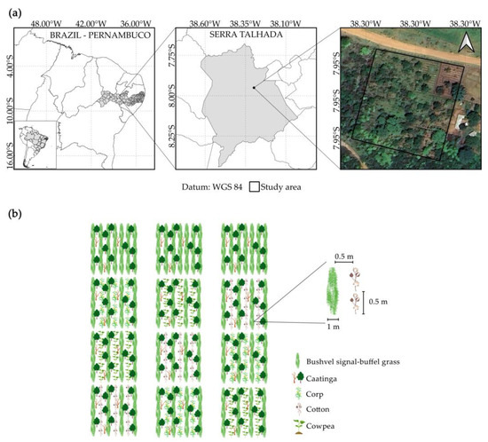
Figure 1.
(a) Location of the experiment, and (b) experimental design.
The experimental area was 7200 m2 (80 m × 90 m), divided into three blocks containing four 584 m2 (29.20 m × 20 m) plots, comprising four agroforestry systems in each block of the area (Figure 1b). The agroforestry systems relied on an integration between the vegetation of the Caatinga biome (Table 1), forage plants, and crops. Bushveld signal grass (Urochloa mosambicensis (Hack.) Dandy) and buffel grass (Cenchrus ciliaris L.) were used, and the crops were as follows: corn (Zea mays L.) cv. Batité, cowpea (Vigna unguiculata (L.) Walp.) cv. CCE-115 and cotton (Gossypium hirsutum L.) cv. BRS Aroeira. The treatments consisted of four agroforestry systems in the Caatinga biome, characterized as follows: (1) bushveld signal–buffel grass + cowpea + Caatinga; (2) bushveld signal–buffel grass + cotton + Caatinga; (3) bushveld signal–buffel grass + corn + Caatinga; and (4) bushveld signal–buffel grass + Caatinga (Figure 1b).

Table 1.
Species found in the experimental area.
In preparing the area, the Caatinga vegetation was thinned and lowered to make the environment more favorable for the development of other crops. The bushveld signal grass and buffel grass were already established in the area before the beginning of the experiment, and a uniform cut was made at a height of 10 cm from the ground with the aid of a backpack brush cutter (Stihl FS160). For planting the crops, 1 m wide and 26 m long planting strips were opened between the grasses, resulting in a gap of 0.5 m between the crops and the grass. The spacing was 0.5 m between plants and 2 m between rows.
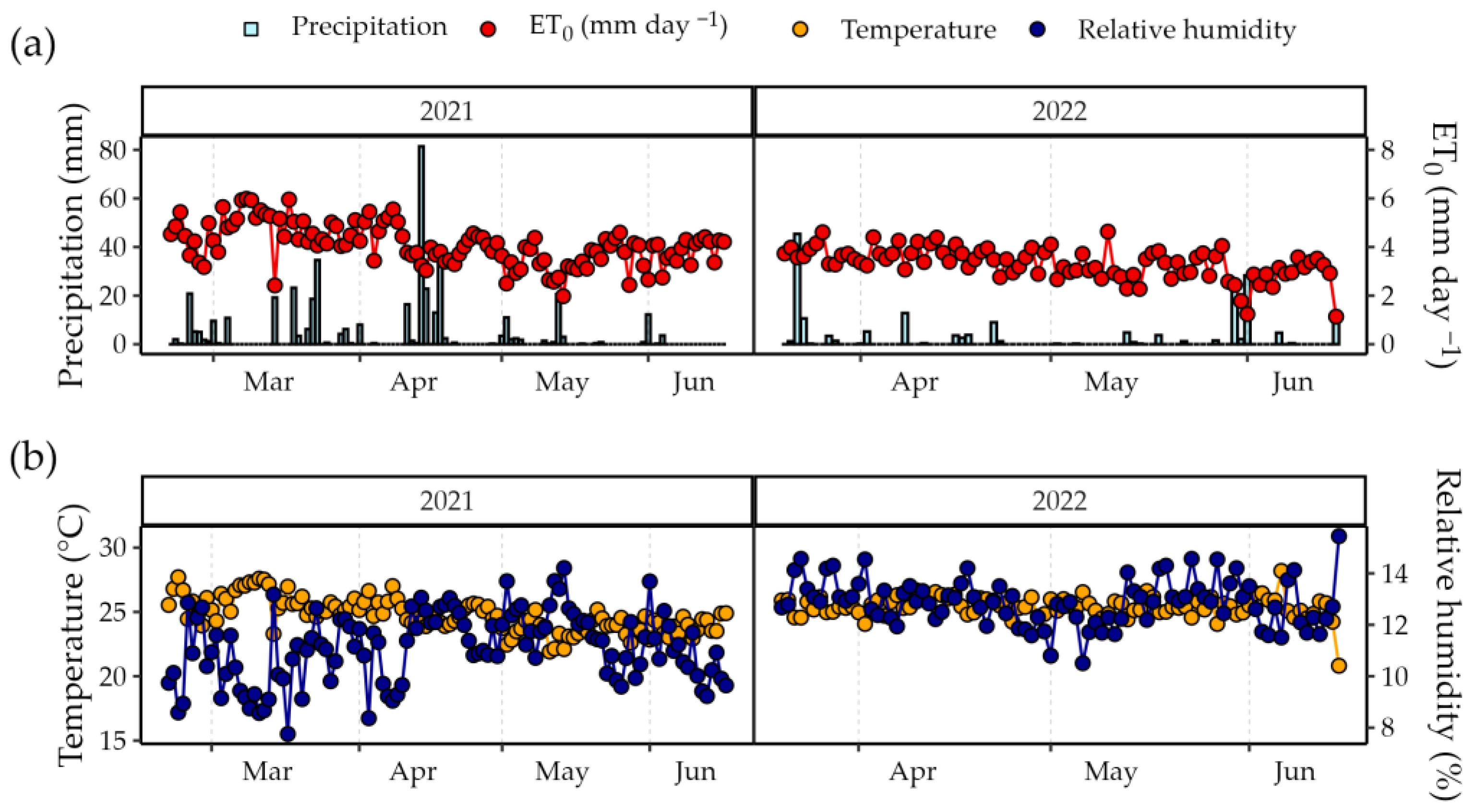
The region is characterized by climate BSwh-type (semiarid climate with dry winters and rainy summers) according to Köppen climate classification [30]. During the experimental period, air temperatures of 24.75 and 25.41 °C, relative humidity of 66.64 and 77.27%, accumulated precipitation of 419.80 and 180.3 mm, accumulated reference evapotranspiration of 483.76 and 292.77 mm, and global solar radiation of 19.02 and 17.01 MJ m−2 were recorded in 2021 and 2022, respectively, obtained from the meteorological station of the National Institute of Meteorology (INMET), located 548 m from the experimental area (Figure 2).
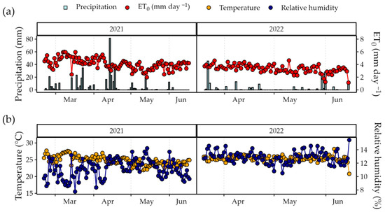
Figure 2.
Meteorological conditions during the experimental period, 26 February 2021 to 17 June 2021 and 25 February 2022 to 29 June 2022. (a) Precipitation and reference evapotranspiration (ET0) values [31]. (b) Air temperature and relative humidity.
2.2. Unmanned Aerial Vehicle Flight Pattern
An advanced DJI Phantom 3 UAV (DJI, Shenzhen, China), equipped with a 1/2.3″ CMOS sensor and 12.76 megapixels (12.4 effective megapixels), was used to capture the images (Figure 3a,b). The flight plan was executed according to the boustrophedon pattern [32] (Figure 3) using the free version of the DroneDeploy software (version 5.31.0). The flight height was maintained at 100 m above the ground, with an 85% overlap at the front and sides. The flight speed was three m s−1, and the total flight time was approximately 6 min. The image overlap pattern, an essential aspect of the image capture process, was set to at least 80% frontal and 70% lateral, following specific recommendations [33]. This meticulous planning minimized information loss. The image coordinates were obtained using the GPS/Glonass global positioning system integrated into the UAV. The images were collected weekly between 10 a.m. and 2 p.m., ensuring consistent illumination and avoiding the presence of clouds. This precaution was taken to prevent interference from shading in the capture area, thus ensuring the quality of the images. No image correction was applied to obtain the reflectance, and the digital image response was used for processing.
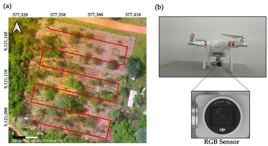
Figure 3.
(a) UAV’s trajectory performed during the flight. (b) UAV platform (DJI Phantom 3) and sensor (CMOS camera, Tokyo Electron Ltd., Tokyo, Japan) used in this study.
2.3. Orthomosaics and Vegetation Indices
The images collected in flight were processed into orthomosaic forms, which consist of building a single image from the composition of overlapping photos [32]. The orthomosaics were processed using WebODM (version 1.9.15) [34], an open-source drone mapping software. After the generation of the orthomosaics, georeferencing corrections were performed using QGIS (version 3.20.10) [35] via the LF Tools plugin. This tool performs georeferencing adjustment through control points on the ground, which were manually determined in the image by selecting known points that remained stationary during the collections, such as roofs and water tanks. Additionally, an affine polynomial function of degree one was adopted for the correction, and the nearest neighbor method was used for interpolation. Thus, after georeferencing adjustment, our orthomosaics were manipulated in R software (version 4.1.3) [36] with the aid of the raster [37] and FIELDimageR [38] packages. The orthomosaics underwent four approaches, Agrofor-Complete; Soil-Removed; Tree-Removed, and Tree + Soil-Removed, as described in Table 2.
Table 2.
Description of the files generated from each orthomosaic.
The removal of the components, soil, and tree was intended to improve the influence of each component on the correlation between the generated vegetation indexes and the parameters to be estimated. No crop removal occurred due to greater difficulty in differentiating the grasses. For soil removal, threshold values of the VARI vegetation index were used, using a cutoff value of −0.16. For the removal of the trees, a cut mask was manually created. Due to the easier identification, the orthomosaic from the beginning of the experiment (Figure 3) was used as a reference, when the crops had not yet been implemented. Subsequently, 11 RGB (Red, Green, Blue)-based vegetation indexes (Table 3) were calculated for each of the generated files (Table 2) on all collection dates.
Table 3.
Descriptive analysis of biomass and leaf area index of buffel grass and bushveld signal grass for each treatment.
2.4. Forage Mass and Leaf Area Index (LAI)
The forage mass and leaf area index of the grasses was determined on days coincident with the collection of images. Forage mass was cut at ground level with a 0.25 m2 frame in three representative points per plot for each grass. Subsequently, the samples were weighed to define the fresh biomass (FB), placed in paper bags, properly identified, and dried in an air-forced circulation oven at 55 °C for 72 h to determine the dry biomass (DB).
Leaf area index (LAI) was obtained using a portable AccuPAR ceptometer sensor (LP-80, Decagon Devices, Pullman, WA, USA) [48], taking five measurements at representative locations per plot, considering the same time interval and light conditions of the image collections.
2.5. Correlation Analysis
The Spearman’s correlation coefficients (ρ) were used to evaluate the correlations between the vegetation indexes and the considered crop parameters (fresh mass, dry mass, and LAI). This method was chosen because of its better ability to assess the degree of association in a scenario of more dispersed data and with the presence of outliers [49,50]. The correlation coefficient values were categorized as very strong (ρ ≥ 0.8), strong (0.6 ≤ ρ < 0.8), moderate (0.4 ≤ ρ < 0.6), weak (0.2 ≤ ρ < 0.4), and very weak (ρ < 0.2). Statistical analysis was performed using R software (version 4.1.3) [36].
2.6. Machine Learning Models
For the machine learning models, the following methods were used: linear regression, which is a statistical method used to determine relationships between a dependent variable (value to be predicted) and one or more independent variables (predictors), assuming a linear relationship between the variables [51]; neural networks (ANNs), which consist of a simplified process inspired by biological neural networks, enabling pattern recognition in complex datasets through learning [52,53]; support vector machines (SVMs), with learning that involves pattern recognition by defining a hyperplane that partitions the data into homogeneous areas, to assist in the prediction processes [25,54]; cubist (Cub), a model tree method characterized by the use of trees for further regression analysis, where regression is applied on the subset of data that are formed after the data partitioning performed by the trees [55]; boosted regression trees (BRTs), notable for their high predictive power when considering the concept of recursive binary splitting in conjunction with a learning (boosting) technique [56]; and classification and regression trees (CARTs), based on rules that allow trees to be created from recursive partitioning, dividing data into subsets based on independent factors [57].
2.7. Model Evaluation
The predictive performance of the models was evaluated using k-fold cross validation, repeated ten times, which consists of dividing the data into subsets, using one of the subsets as a test and the others to estimate the model, increasing reliability and unbiasedness during estimation [58]. The following were used to evaluate the cross-validation results: the root mean square error (RMSE), the mean absolute error (MAE), Lin’s concordance correlation coefficient (CCC), and the coefficient of determination (R2).
The modeling process was performed with R software version 4.1.3 [36], with the aid of the packages neuralnet [59], kernlab [60], Cubist [61], gbm [62], and rpart [63] for the ANNs, SVM, Cub, BRTs, and CART models, respectively. The packages caret [64] and DescTools [65] were used for evaluation.
3. Results
3.1. Correlating and Determining the Orthomosaic Treatment Approach
As in the results, there was no difference between the treatments performed; all images and the yield variables (FB, DB, and LAI) were evaluated together, that is, independent of the agroforestry systems. The average, maximum, minimum, median, and standard deviation data are described (Table 4).
Table 4.
Descriptive analysis of biomass and leaf area index of buffel grass and bushveld signal grass for each treatment.
The NGRDI, MGRVI, and VARI indexes showed the highest positive and significant (p < 0.05) correlations for fresh mass (0.8 for NGRDI, 0.8 for MGRVI, and 0.8 for VARI), dry mass (0.7 for NGRDI, 0.7 for MGRVI, and 0.7 for VARI), and LAI (0.7 for NGRDI 0.7 for MGRDI, and 0.7 for VARI), respectively. The SCI, SI, and * HUE indexes showed the highest negative and significant (p < 0.05) correlations for fresh biomass (0.8 for SCI, 0.7 for SI, and 0.7 for * HUE), dry mass (0.7 for SCI, 0.7 for SI, and 0.7 for * HUE), and LAI (0.7 for SCI, 0.6 for SI, and 0.5 for * HUE), respectively, while BGI, GLI, RGB, and BI showed non-significant occurrences (p > 0.05) (Figure 4). The indexes SCI and MGRVI showed significant behavior (p < 0.05) identical to NGRDI with correlations of 0.8, 0.7, and 0.7 for FB, DB, and LAI, respectively, with SCI values in modulo equal to the values of NGRDI. It was decided to remove both in the estimation process, keeping only the NGRDI (Figure 4).

Figure 4.
Spearman’s correlation coefficients of the relationship between the considered features and the vegetation indexes for each approach on orthomosaics. The asterisk (*) represents a statistically significant difference (p < 0.05). (a) Original file containing all components of the study area (soil, crops, trees). (b) File with soil and tree components removed. (c) File with tree component removed. (d) File with solo component removed.
The approach to treating the orthomosaics by removing components (tree and soil) that contributed the most to improving correlation values was the removal of trees (Figure 4) and was used in generating the predictive models.
3.2. Analysis of Prediction Models
Regarding the linear regression models, the NGRDI showed a better fit for FB (RMSE = 4002.04, MAE = 3551.13, CCC = 0.83, R2 = 0.75) and DB (RMSE = 1743.56, MAE = 1514.18, CCC = 0.71, R2 = 0.69), and the VARI for LAI (RMSE = 0.31, MAE = 0.26, CCC = 0.77, R2 = 0.71), in which it showed a less obvious difference between the indexes than for FB and DB (Table 5).
Table 5.
Results of the cross-validation process for the simple linear regression models.
For the machine learning methods, the best models were found for the partitioned regression tree method (Table 6), even compared to linear regression (Table 5), presenting a lower RMSE, that is, with values of 3020.86, 1201.75, and 0.20 for FB, DB, and LAI, respectively, as well as higher precision and accuracy for the predicted values (CCC), presenting values of 0.94 for FB, DB, and LAI.
Table 6.
Results of the cross-validation process for the machine learning methods.
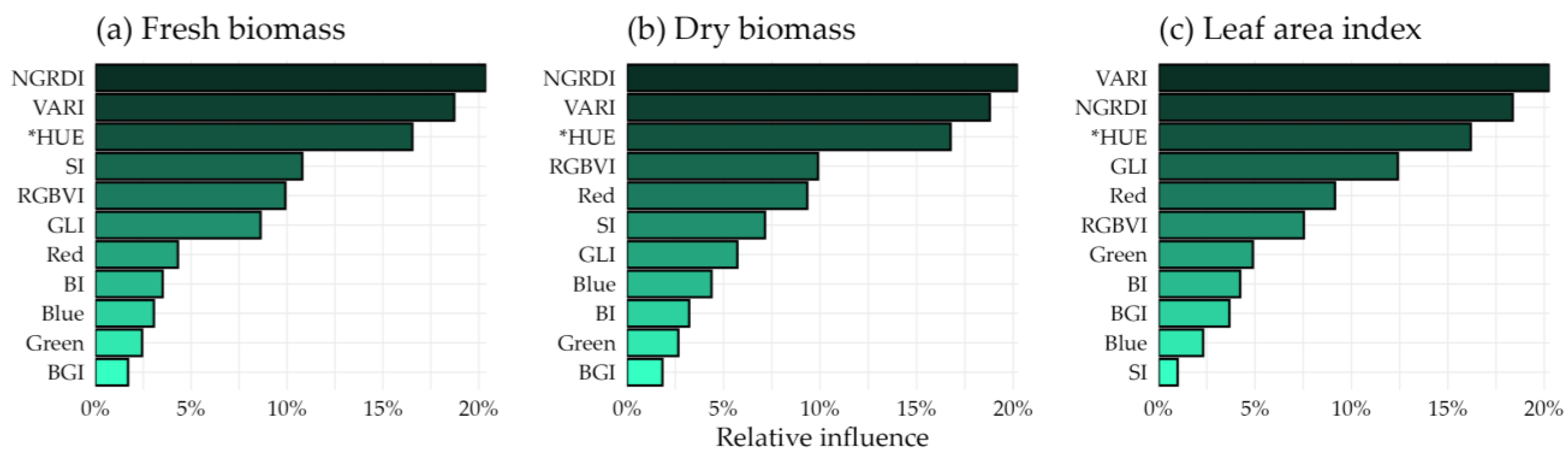
Analyzing the influences of the variables in the CART prominence model, one notices that NGRDI and VARI are prominent, as well as in the linear correlation indexes (Figure 5), followed by the * HUE index.
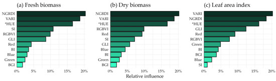
Figure 5.
The relative influence of the indexes on the final classification and regression tree (CART) models. (a) Fresh biomass, (b) dry biomass, and (c) leaf area index.
4. Discussion
Removing the trees from the orthomosaics for the estimation process proved important in predicting the production variables of bushveld signal grass and buffel grass in agroforestry systems in the Caatinga biome, similar to that found by [66] in their analysis of aboveground tree biomass in an agroforestry system, where only the trees were extracted for model generation. The removal of the trees in this study was superior even when compared to the removal of the trees together with the ground surface. This is possibly because the ground surface acts as a balance to the high values that occur due to saturation problems of the indexes, occasioned in denser canopy conditions [67], as the ground values are represented by values near or below zero by most indexes. Therefore, removing the soil from the orthomosaics would potentiate the saturation problem of the RGB sensor products, compromising the estimation of the yield parameters, reinforced by the considerable influence of the * HUE soil index on the best-performing CART model (Figure 5).
The MGRVI, developed by [44] from the NGRDI, with the premise that the squared elevation of the reflectances used in generating the indexes contributes to amplifying the difference between them, showed identical behavior to that visualized for the NGRDI. That demonstrates that in this experiment, no influence of squared elevation was observed in the association with the analyzed elements, characterizing this process as irrelevant in the prediction models, different from [68], where NGRDI was better in the process of extracting the vegetation of Haloxylon ammodendron compared to MGRVI. As for the SCI, developed based on the variation in the soil tone [46], it is exactly the inverse of the NGRDI and contributes solely to visual aspects that could be obtained by inverting the final NGRDI values or even the color scale used.
The generally superior predictive performance of NGRDI (FB and DB) followed by VARI (LAI) (see Table 5 and Figure 5) corresponds to the various studies in the literature that relate it to biomass, such as [69], who described NGRDI as efficient in identifying biomass and yield and capturing small differences in chlorophyll content of the corn crop. Ref. [70] found an optimal correlation of NGRDI with alfalfa biomass. Ref. [71] also found excellent contributions of the VARI in their models, highlighting the predictive ability even in shadier conditions, thus denoting the capability of these indexes even in the most adverse situations inherent to remote sensing data collection. Unlike the relationships presented by [72] evaluating the severity of diseases on leaves under controlled conditions in image taking, few indexes showed a strong relationship with the adjusted parameters, demonstrating the influence of environmental and physical conditions imposed during image taking, either by meteorological issues, the inclination of the sun, or even by the complexity of the production field. In any case, the satisfactory ratio shown by NGRDI and VARI may be related to the greater focus, of their respective formulas, on the red and green bands, as they have a higher quantum yield and a higher reflection rate, respectively [73,74,75].
The linear regression models, with a model that is easier to reproduce, and the other models generated, although they showed a worse performance than CART, can still be used. According to [76], even under conditions where precision and accuracy are not obtained, the methods can still be recommended due to the cost, the time-consuming and destructive measurements, and the producer’s experience in their area. The models developed presented satisfactory predictive performance with considerably high accuracy and precision, given the various factors that influence the estimation process, such as environmental conditions, the complexity of vegetation, equipment, and the quality of the data survey [77]. The better performance of the CART method, as per the calculated values of CCC (0.94) and R2 (0.89), is due to factors such as the ability to leverage information through learning, being robust to the outlier, non-parametric, and, most importantly, being less sensitive to learning data [78]. It is important to highlight that unfavorable weather conditions have resulted in insufficient yields of cowpea, corn, and cotton crops, limiting the consideration of their impact on the system during the modeling process. Therefore, it is important to conduct research that takes these factors into account to make significant advances in estimative methods in AFS. Furthermore, the process of removing components from orthomosaics through threshold values or cutting masks is still performed manually, which can lead to a prolonged process in large-scale applications, particularly in the removal of trees involving variable structures. Therefore, it is crucial to develop automated algorithms for such tasks, considering precision and process optimization.
5. Conclusions
In this study, different vegetation indices and algorithms were used for modeling the biomass and leaf area index of forage crops (common grass and buffel grass) in agroforestry systems in the Caatinga biome. Additionally, the removal of system components (trees and soils) was performed to improve the accuracy of the models. Based on the presented results, we suggest employing regression tree-based models (CART) as a viable option when constructing predictive models for biomass and leaf area index of common grass and buffel grass in agroforestry systems within the Caatinga biome.
The robustness of these models, evidenced by their ability to handle outliers and their relative insensitivity to training data, makes them suitable for the complexity of the conditions found in this environment. Furthermore, the simplicity and ease of replication of linear regression-based models, particularly when using indices like NGRDI and VARI, make them a viable option for estimating productive indices in these conditions. It is also worth emphasizing the importance of tree removal from orthomosaics as a significant procedure in predicting both evaluated modeling methods.
Author Contributions
Conceptualization, A.C.B., E.J.O.d.S. and W.M.d.S.; methodology, A.C.B., C.d.J.P.C., D.M.J., E.J.O.d.S., J.C.B.D.J. and W.M.d.S.; software, A.C.B., A.M.d.R.F.J., E.J.O.d.S. and W.M.d.S.; validation, A.M.d.R.F.J., J.C.B.D.J., M.L.d.S.M. and M.V.d.C.; formal analysis, D.M.J., E.J.O.d.S., J.C.B.D.J., M.V.d.C. and W.M.d.S.; investigation, A.C.B., C.d.J.P.C., E.J.O.d.S., J.C.B.D.J., M.L.d.S.M. and W.M.d.S.; resources, A.C.B., D.M.J., E.J.O.d.S., J.C.B.D.J. and M.V.d.C.; data curation, A.C.B., C.d.J.P.C., E.J.O.d.S., M.L.d.S.M. and W.M.d.S.; writing—original draft preparation, A.C.B., C.d.J.P.C., E.J.O.d.S., M.L.d.S.M. and W.M.d.S.; writing—review and editing, A.M.d.R.F.J., D.M.J., J.C.B.D.J. and M.V.d.C.; visualization, A.C.B., A.M.d.R.F.J., E.J.O.d.S. and W.M.d.S.; supervision, E.J.O.d.S. and J.C.B.D.J.; project administration, E.J.O.d.S., J.C.B.D.J. and W.M.d.S.; funding acquisition, E.J.O.d.S., J.C.B.D.J. and M.V.d.C. All authors have read and agreed to the published version of the manuscript.
Funding
Financial support was provided by the Foundation for the Support of Science and Technology of the State of Pernambuco (FACEPE) under grants IBPG-1035-5.01/21. The authors would like to thank the Coordination for the Improvement of Higher Education Personnel (CAPES) under the Finance Code 001. A.M.d.R.F.J. acknowledges support from the São Paulo Research Foundation—FAPESP grant 2023/05323-4. M.V.d.C. acknowledges a scholarship from the National Council for Scientific and Technological Development—CNPq.
Institutional Review Board Statement
Not applicable.
Informed Consent Statement
Not applicable.
Data Availability Statement
The original contributions presented in the study are included in the article, further inquiries can be directed to the corresponding author.
Acknowledgments
We thank the Section Managing Editor, Damaris Zhao, and three anonymous reviewers for their insightful comments and suggestions on the manuscript.
Conflicts of Interest
The authors declare no conflicts of interest.
References
- Oliveira, V.R.; e Silva, P.S.L.; de Paiva, H.N.; Pontes, F.S.T.; Antonio, R.P. Growth of Arboreal Leguminous Plants and Maize Yield in Agroforestry Systemsm. Rev. Arvore 2016, 40, 679–688. [Google Scholar] [CrossRef]
- Queiroz, M.G.; da Silva, T.G.F.; de Souza, C.A.A.; da Rosa Ferraz Jardim, A.M.; do Nascimento Araújo, G.; de Souza, L.S.B.; de Moura, M.S.B. Composition of Caatinga Species under Anthropic Disturbance and Its Correlation with Rainfall Partitioning. Floresta E Ambient. 2021, 28, e20190044. [Google Scholar] [CrossRef]
- Carvalho, W.F.; Alves, A.A.; Pompeu, R.C.F.F.; Araújo, A.R.; Fernandes, F.É.P.; dos Santos Costa, C.; de Sousa Oliveira, D.; Memória, H.Q.; Guedes, L.F.; Muir, J.P.; et al. Effect of Concentrate Supplement to Ewes on Nutritive Value of Ingested Caatinga Native Forage Nutritive Value as Affected by Season. Trop. Anim. Health Prod. 2021, 53, 556. [Google Scholar] [CrossRef] [PubMed]
- de Queiroz, M.G.; da Silva, T.G.F.; Zolnier, S.; Jardim, A.M.D.R.F.; de Souza, C.A.A.; Júnior, G.D.N.A.; de Morais, J.E.F.; de Souza, L.S.B. Spatial and Temporal Dynamics of Soil Moisture for Surfaces with a Change in Land Use in the Semi-Arid Region of Brazil. Catena 2020, 188, 104457. [Google Scholar] [CrossRef]
- Pinheiro, F.M.; Nair, P.K.R. Silvopasture in the Caatinga Biome of Brazil: A Review of Its Ecology, Management, and Development Opportunities. For. Syst. 2018, 27, eR01S. [Google Scholar] [CrossRef]
- Sharma, P.; Bhardwaj, D.R.; Singh, M.K.; Nigam, R.; Pala, N.A.; Kumar, A.; Verma, K.; Kumar, D.; Thakur, P. Geospatial Technology in Agroforestry: Status, Prospects, and Constraints. Environ. Sci. Pollut. Res. 2022, 30, 116459–116487. [Google Scholar] [CrossRef] [PubMed]
- Suárez, L.R.; Suárez Salazar, J.C.; Casanoves, F.; Ngo Bieng, M.A. Cacao Agroforestry Systems Improve Soil Fertility: Comparison of Soil Properties between Forest, Cacao Agroforestry Systems, and Pasture in the Colombian Amazon. Agric. Ecosyst. Environ. 2021, 314, 107349. [Google Scholar] [CrossRef]
- Carneiro, F.M.; Angeli Furlani, C.E.; Zerbato, C.; Candida de Menezes, P.; da Silva Gírio, L.A.; Freire de Oliveira, M. Comparison between Vegetation Indices for Detecting Spatial and Temporal Variabilities in Soybean Crop Using Canopy Sensors. Precis. Agric. 2020, 21, 979–1007. [Google Scholar] [CrossRef]
- Xiao, J.; Xiong, K. A Review of Agroforestry Ecosystem Services and Its Enlightenment on the Ecosystem Improvement of Rocky Desertification Control. Sci. Total Environ. 2022, 852, 158538. [Google Scholar] [CrossRef]
- DiMaggio, A.M.; Perotto-Baldivieso, H.L.; Ortega-S, J.A.; Walther, C.; Labrador-Rodriguez, K.N.; Page, M.T.; Martinez, J.D.L.L.; Rideout-Hanzak, S.; Hedquist, B.C.; Wester, D.B. A Pilot Study to Estimate Forage Mass from Unmanned Aerial Vehicles in a Semi-Arid Rangeland. Remote Sens. 2020, 12, 2431. [Google Scholar] [CrossRef]
- Andrade, T.G.; Junior, A.S.D.A.; Souza, M.O.; Lopes, J.W.B.; Vieira, P.F.D.M.J. Soybean Yield Prediction Using Remote Sensing in Southwestern Piauí State, Brazil. Rev. Caatinga 2022, 35, 105–116. [Google Scholar] [CrossRef]
- Arenas-Corraliza, M.G.; López-Díaz, M.L.; Rolo, V.; Cáceres, Y.; Moreno, G. Phenological, Morphological and Physiological Drivers of Cereal Grain Yield in Mediterranean Agroforestry Systems. Agric. Ecosyst. Environ. 2022, 340, 108158. [Google Scholar] [CrossRef]
- Beniaich, A.; Silva, M.L.N.; Guimarães, D.V.; Avalos, F.A.P.; Terra, F.S.; Menezes, M.D.; Avanzi, J.C.; Cândido, B.M. UAV-Based Vegetation Monitoring for Assessing the Impact of Soil Loss in Olive Orchards in Brazil. Geoderma Reg. 2022, 30, e00543. [Google Scholar] [CrossRef]
- Freitas, R.G.; Pereira, F.R.S.; Dos Reis, A.A.; Magalhães, P.S.G.; Figueiredo, G.K.D.A.; do Amaral, L.R. Estimating Pasture Aboveground Biomass under an Integrated Crop-Livestock System Based on Spectral and Texture Measures Derived from UAV Images. Comput. Electron. Agric. 2022, 198, 107122. [Google Scholar] [CrossRef]
- Xue, J.; Su, B. Significant Remote Sensing Vegetation Indices: A Review of Developments and Applications. J. Sens. 2017, 2017, 1353691. [Google Scholar] [CrossRef]
- Castro, R. Remote Monitoring of Coffee Cultivation through Computational Processing of Satellite Images. In Proceedings of the 2019 7th International Engineering, Sciences and Technology Conference (IESTEC), Panama City, Panama, 9–11 October 2019; pp. 13–18. [Google Scholar] [CrossRef]
- Giuffrida, M.V.; Klapp, I.; Huang, J.; Sangjan, W.; Mcgee, R.J.; Sankaran, S. Optimization of UAV-Based Imaging and Image Processing Orthomosaic and Point Cloud Approaches for Estimating Biomass in a Forage Crop. Remote Sens. 2022, 14, 2396. [Google Scholar] [CrossRef]
- Wengert, M.; Piepho, H.P.; Astor, T.; Graß, R.; Wijesingha, J.; Wachendorf, M. Assessing Spatial Variability of Barley Whole Crop Biomass Yield and Leaf Area Index in Silvoarable Agroforestry Systems Using UAV-Borne Remote Sensing. Remote Sens. 2021, 13, 2751. [Google Scholar] [CrossRef]
- Azadbakht, M.; Ashourloo, D.; Aghighi, H.; Homayouni, S.; Shahrabi, H.S.; Matkan, A.A.; Radiom, S. Alfalfa Yield Estimation Based on Time Series of Landsat 8 and PROBA-V Images: An Investigation of Machine Learning Techniques and Spectral-Temporal Features. Remote Sens. Appl. Soc. Environ. 2022, 25, 100657. [Google Scholar] [CrossRef]
- Cosenza, D.N.; Vogel, J.; Broadbent, E.N.; Silva, C.A. Silvicultural Experiment Assessment Using Lidar Data Collected from an Unmanned Aerial Vehicle. For. Ecol. Manag. 2022, 522, 120489. [Google Scholar] [CrossRef]
- Kaushal, R.; Islam, S.; Tewari, S.; Tomar, J.M.S.; Thapliyal, S.; Madhu, M.; Trinh, T.L.; Singh, T.; Singh, A.; Durai, J. An Allometric Model-Based Approach for Estimating Biomass in Seven Indian Bamboo Species in Western Himalayan Foothills, India. Sci. Rep. 2022, 12, 7527. [Google Scholar] [CrossRef]
- Kearney, S.P.; Porensky, L.M.; Augustine, D.J.; Gaffney, R.; Derner, J.D. Monitoring Standing Herbaceous Biomass and Thresholds in Semiarid Rangelands from Harmonized Landsat 8 and Sentinel-2 Imagery to Support within-Season Adaptive Management. Remote Sens. Environ. 2022, 271, 112907. [Google Scholar] [CrossRef]
- Swayze, N.C.; Tinkham, W.T.; Creasy, M.B.; Vogeler, J.C.; Hoffman, C.M.; Hudak, A.T. Influence of UAS Flight Altitude and Speed on Aboveground Biomass Prediction. Remote Sens. 2022, 14, 1989. [Google Scholar] [CrossRef]
- Li, D.; Li, X.; Xi, B.; Hernandez-Santana, V. Evaluation of Method to Model Stomatal Conductance and Its Use to Assess Biomass Increase in Poplar Trees. Agric. Water Manag. 2022, 259, 107228. [Google Scholar] [CrossRef]
- Bawa, A.; Samanta, S.; Himanshu, S.K.; Singh, J.; Kim, J.J.; Zhang, T.; Chang, A.; Jung, J.; DeLaune, P.; Bordovsky, J.; et al. A Support Vector Machine and Image Processing Based Approach for Counting Open Cotton Bolls and Estimating Lint Yield from UAV Imagery. Smart Agric. Technol. 2023, 3, 100140. [Google Scholar] [CrossRef]
- De Graeve, M.; Birse, N.; Hong, Y.; Elliott, C.T.; Hemeryck, L.Y.; Vanhaecke, L. Multivariate versus Machine Learning-Based Classification of Rapid Evaporative Ionisation Mass Spectrometry Spectra towards Industry Based Large-Scale Fish Speciation. Food Chem. 2023, 404, 134632. [Google Scholar] [CrossRef] [PubMed]
- Durmuş, Y.; Atasoy, A.F. Application of Multivariate Machine Learning Methods to Investigate Organic Compound Content of Different Pepper Spices. Food Biosci. 2023, 51, 102216. [Google Scholar] [CrossRef]
- Shi, H.; Yang, D.; Tang, K.; Hu, C.; Li, L.; Zhang, L.; Gong, T.; Cui, Y. Explainable Machine Learning Model for Predicting the Occurrence of Postoperative Malnutrition in Children with Congenital Heart Disease. Clin. Nutr. 2022, 41, 202–210. [Google Scholar] [CrossRef]
- Servia, H.; Pareeth, S.; Michailovsky, C.I.; de Fraiture, C.; Karimi, P. Operational Framework to Predict Field Level Crop Biomass Using Remote Sensing and Data Driven Models. Int. J. Appl. Earth Obs. Geoinf. 2022, 108, 102725. [Google Scholar] [CrossRef]
- Alvares, C.A.; Stape, J.L.J.L.; Sentelhas, P.C.; Leonardo, J.; Gonçalves, M.; Stape, J.L.J.L.; Sparovek, G.; De Moraes Gonçalves, J.L.; Sparovek, G. Köppen’s Climate Classification Map for Brazil. Meteorol. Z. 2013, 22, 711–728. [Google Scholar] [CrossRef]
- Allen, R.G.; Pereira, L.S.; Raes, D.; Smith, M. Crop Evapotranspiration—Guidelines for Computing Crop Water Requirements. In FAO Irrigation and Dranaige; FAO, Ed.; FAO—Food and Agriculture Organization of the United Nations: Roma, Italy, 1998; p. 56. ISBN 92-5-104219-5. [Google Scholar]
- Rossello, N.B.; Carpio, R.F.; Gasparri, A.; Garone, E. Information-Driven Path Planning for UAV With Limited Autonomy in Large-Scale Field Monitoring. IEEE Trans. Autom. Sci. Eng. 2021, 19, 2450–2460. [Google Scholar] [CrossRef]
- Arantes, B.H.T.; Arantes, L.T.; Costa, E.M.; Ventura, M.V.A. Drone Aplicado Na Agricultura Digital. Ipê Agron. J. 2019, 3, 14–18. [Google Scholar] [CrossRef]
- WebODM. WebODM Drone Mapping Software. OpenDroneMap. Available online: https://www.opendronemap.org/webodm/ (accessed on 10 January 2021).
- QGIS Development Team. QGIS Geographic Information System. Available online: https://qgis.org/ro/site (accessed on 10 January 2024).
- R Core Team. R: A Language and Environment for Statistical Computing; R Foundation for Statistical Computing: Vienna, Austria, 2024; Available online: https://www.R-project.org/ (accessed on 10 January 2024).
- Hijmans, R. Raster: Geographic Data Analysis and Modeling. R Package Version 3.6-26. 2023. Available online: https://CRAN.R-project.org/package=raster (accessed on 10 January 2024).
- Matias, F.I.; Caraza-Harter, M.V.; Endelman, J.B. FIELDimageR: An R Package to Analyze Orthomosaic Images from Agricultural Field Trials. Plant Phenome J. 2020, 3, e20005. [Google Scholar] [CrossRef]
- Richardson, A.J.; Weigand, C.L. Distinguishing Vegetation from Soil Background Information. Photogramm. Eng. Remote Sens. 1977, 43, 1541–1552. [Google Scholar]
- Zarco-Tejada, P.J.; Berjón, A.; López-Lozano, R.; Miller, J.R.; Martín, P.; Cachorro, V.; González, M.R.; De Frutos, A. Assessing Vineyard Condition with Hyperspectral Indices: Leaf and Canopy Reflectance Simulation in a Row-Structured Discontinuous Canopy. Remote Sens. Environ. 2005, 99, 271–287. [Google Scholar] [CrossRef]
- Louhaichi, M.; Borman, M.M.; Johnson, D.E. Spatially Located Platform and Aerial Photography for Documentation of Grazing Impacts on Wheat. Geocarto Int. 2001, 16, 65–70. [Google Scholar] [CrossRef]
- Escadafal, R.; Belghit, R.; Ben-Moussa, A. Indices Spectraux Pour La Télédétection de La Dégradation Des Milieux Naturels En Tunisie Aride. In Proceedings of the 6th International Symposium on Physical Measurements and Signatures in Remote Sensing, Val-d’Isère, France, 17–21 January 1994; pp. 17–21. [Google Scholar]
- Tucker, C.J. Red and Photographic Infrared Linear Combinations for Monitoring Vegetation. Remote Sens. Environ. 1979, 8, 127–150. [Google Scholar] [CrossRef]
- Bendig, J.; Yu, K.; Aasen, H.; Bolten, A.; Bennertz, S.; Broscheit, J.; Gnyp, M.L.; Bareth, G. Combining UAV-Based Plant Height from Crop Surface Models, Visible, and near Infrared Vegetation Indices for Biomass Monitoring in Barley. Int. J. Appl. Earth Obs. Geoinf. 2015, 39, 79–87. [Google Scholar] [CrossRef]
- Possoch, M.; Bieker, S.; Hoffmeister, D.; Bolten, A.; Schellberg, J.; Bareth, G. Multi-Temporal Crop Surface Models Combined with the RGB Vegetation Index from UAV-Based Images for Forage Monitoring in Grassland. Int. Arch. Photogramm. Remote Sens. Spat. Inf. Sci. 2016, 41, 991–998. [Google Scholar] [CrossRef]
- Mathieu, R.; Pouget, M.; Cervelle, B.; Escadafal, R. Relationships between Satellite-Based Radiometric Indices Simulated Using Laboratory Reflectance Data and Typic Soil Color of an Arid Environment. Remote Sens. Environ. 1998, 66, 17–28. [Google Scholar] [CrossRef]
- Gitelson, A.A.; Kaufman, Y.J.; Stark, R.; Rundquist, D. Novel Algorithms for Remote Estimation of Vegetation Fraction. Remote Sens. Environ. 2002, 80, 76–87. [Google Scholar] [CrossRef]
- Fang, H.; Li, W.; Wei, S.; Jiang, C. Seasonal Variation of Leaf Area Index (LAI) over Paddy Rice Fields in NE China: Intercomparison of Destructive Sampling, LAI-2200, Digital Hemispherical Photography (DHP), and AccuPAR Methods. Agric. For. Meteorol. 2014, 198, 126–141. [Google Scholar] [CrossRef]
- Schober, P.; Schwarte, L.A. Correlation Coefficients: Appropriate Use and Interpretation. Anesth. Analg. 2018, 126, 1763–1768. [Google Scholar] [CrossRef] [PubMed]
- Winter, J.C.F.; Gosling, S.D.; Potter, J. Comparing the Pearson and Spearman Correlation Coefficients across Distributions and Sample Sizes: A Tutorial Using Simulations and Empirical Data. Psychol. Methods 2016, 21, 273–290. [Google Scholar] [CrossRef] [PubMed]
- Wang, Y.; Shi, W.; Wen, T. Prediction of Winter Wheat Yield and Dry Matter in North China Plain Using Machine Learning Algorithms for Optimal Water and Nitrogen Application. Agric. Water Manag. 2023, 277, 108140. [Google Scholar] [CrossRef]
- Gue, I.H.V.; Ubando, A.T.; Tseng, M.L.; Tan, R.R. Artificial Neural Networks for Sustainable Development: A Critical Review. Clean Technol. Environ. Policy 2020, 22, 1449–1465. [Google Scholar] [CrossRef]
- Hasson, U.; Nastase, S.A.; Goldstein, A. Direct Fit to Nature: An Evolutionary Perspective on Biological and Artificial Neural Networks. Neuron 2020, 105, 416–434. [Google Scholar] [CrossRef] [PubMed]
- Mousavizadegan, M.; Hosseini, M.; Sheikholeslami, M.N.; Hamidipanah, Y.; Reza Ganjali, M. Smartphone Image Analysis-Based Fluorescence Detection of Tetracycline Using Machine Learning. Food Chem. 2023, 403, 134364. [Google Scholar] [CrossRef] [PubMed]
- Alabi, T.R.; Abebe, A.T.; Chigeza, G.; Fowobaje, K.R. Estimation of Soybean Grain Yield from Multispectral High-Resolution UAV Data with Machine Learning Models in West Africa. Remote Sens. Appl. Soc. Environ. 2022, 27, 100782. [Google Scholar] [CrossRef]
- Döpke, J.; Fritsche, U.; Pierdzioch, C. Predicting Recessions with Boosted Regression Trees. Int. J. Forecast. 2017, 33, 745–759. [Google Scholar] [CrossRef]
- Pourghasemi, H.R.; Rahmati, O. Prediction of the Landslide Susceptibility: Which Algorithm, Which Precision? Catena 2018, 162, 177–192. [Google Scholar] [CrossRef]
- Tajik, S.; Ayoubi, S.; Zeraatpisheh, M. Digital Mapping of Soil Organic Carbon Using Ensemble Learning Model in Mollisols of Hyrcanian Forests, Northern Iran. Geoderma Reg. 2020, 20, e00256. [Google Scholar] [CrossRef]
- Fritsch, S.; Guenther, F.; Wright, M. Neuralnet: Training of Neural Networks. R Package Version 1.44.2. 2019. Available online: https://CRAN.R-project.org/package=neuralnet (accessed on 10 January 2024).
- Karatzoglou, A.; Hornik, K.; Smola, A.; Zeileis, A. Kernlab—An S4 Package for Kernel Methods in R. J. Stat. Softw. 2004, 11, 1–20. [Google Scholar] [CrossRef]
- Kuhn, M.; Quinlan, R. Cubist: Rule-and Instance-Based Regression Modeling. R Package Version 0.4.2.1. 2023. Available online: https://CRAN.R-project.org/package=Cubist (accessed on 10 January 2024).
- Greg, R.; Developers, G. gbm: Generalized Boosted Regression Models. R Package Version 2.1.9. 2024. Available online: https://CRAN.R-project.org/package=gbm (accessed on 10 January 2024).
- Therneau, T.; Atkinson, B. rpart: Recursive Partitioning and Regression Trees. R Package Version 4.1.23. 2023. Available online: https://CRAN.R-project.org/package=rpart (accessed on 10 January 2024).
- Kuhn, M. Building Predictive Models in R Using the Caret Package. J. Stat. Softw. 2008, 28, 1–26. [Google Scholar] [CrossRef]
- Signorell, A. DescTools: Tools for Descriptive Statistics. R Package Version 0.99.54. 2024. Available online: https://CRAN.R-project.org/package=DescTools (accessed on 10 January 2024).
- Lourenço, P.; Godinho, S.; Sousa, A.; Gonçalves, A.C. Estimating Tree Aboveground Biomass Using Multispectral Satellite-Based Data in Mediterranean Agroforestry System Using Random Forest Algorithm. Remote Sens. Appl. Soc. Environ. 2021, 23, 100560. [Google Scholar] [CrossRef]
- Cao, Z.; Cheng, T.; Ma, X.; Tian, Y.; Zhu, Y.; Yao, X.; Chen, Q.; Liu, S.; Guo, Z.; Zhen, Q.; et al. A New Three-Band Spectral Index for Mitigating the Saturation in the Estimation of Leaf Area Index in Wheat. Int. J. Remote Sens. 2017, 38, 3865–3885. [Google Scholar] [CrossRef]
- Xu, J.; Gu, H.; Meng, Q.; Cheng, J.; Liu, Y.; Jiang, P.; Sheng, J.; Deng, J.; Bai, X. Spatial Pattern Analysis of Haloxylon Ammodendron Using UAV Imagery—A Case Study in the Gurbantunggut Desert. Int. J. Appl. Earth Obs. Geoinf. 2019, 83, 101891. [Google Scholar] [CrossRef]
- Elazab, A.; Ordóñez, R.A.; Savin, R.; Slafer, G.A.; Araus, J.L. Detecting Interactive Effects of N Fertilization and Heat Stress on Maize Productivity by Remote Sensing Techniques. Eur. J. Agron. 2016, 73, 11–24. [Google Scholar] [CrossRef]
- Tang, Z.; Parajuli, A.; Chen, C.J.; Hu, Y.; Revolinski, S.; Medina, C.A.; Lin, S.; Zhang, Z.; Yu, L.X. Validation of UAV-Based Alfalfa Biomass Predictability Using Photogrammetry with Fully Automatic Plot Segmentation. Sci. Rep. 2021, 11, 3336. [Google Scholar] [CrossRef] [PubMed]
- Sapkota, B.; Singh, V.; Neely, C.; Rajan, N.; Bagavathiannan, M. Detection of Italian Ryegrass in Wheat and Prediction of Competitive Interactions Using Remote-Sensing and Machine-Learning Techniques. Remote Sens. 2020, 12, 2977. [Google Scholar] [CrossRef]
- Alves, K.S.; Guimarães, M.; Ascari, J.P.; Queiroz, M.F.; Alfenas, R.F.; Mizubuti, E.S.G.; Del Ponte, E.M. RGB-Based Phenotyping of Foliar Disease Severity under Controlled Conditions. Trop. Plant Pathol. 2022, 47, 105–117. [Google Scholar] [CrossRef]
- Hogewoning, S.W.; Wientjes, E.; Douwstra, P.; Trouwborst, G.; van Ieperen, W.; Croce, R.; Harbinson, J. Photosynthetic Quantum Yield Dynamics: From Photosystems to Leaves. Plant Cell 2012, 24, 1921–1935. [Google Scholar] [CrossRef] [PubMed]
- Kume, A. Importance of the Green Color, Absorption Gradient, and Spectral Absorption of Chloroplasts for the Radiative Energy Balance of Leaves. J. Plant Res. 2017, 130, 501–514. [Google Scholar] [CrossRef] [PubMed]
- Zhen, S.; van Iersel, M.W. Far-Red Light Is Needed for Efficient Photochemistry and Photosynthesis. J. Plant Physiol. 2017, 209, 115–122. [Google Scholar] [CrossRef] [PubMed]
- Rotz, S.; Duncan, E.; Small, M.; Botschner, J.; Dara, R.; Mosby, I.; Reed, M.; Fraser, E.D.G. The Politics of Digital Agricultural Technologies: A Preliminary Review. Sociol. Ruralis 2019, 59, 203–229. [Google Scholar] [CrossRef]
- Colaço, A.F.; Trevisan, R.G.; Karp, F.H.S.; Molin, J.P. Yield Mapping Methods for Manually Harvested Crops. Comput. Electron. Agric. 2020, 177, 105693. [Google Scholar] [CrossRef]
- Choubin, B.; Zehtabian, G.; Azareh, A.; Rafiei-Sardooi, E.; Sajedi-Hosseini, F.; Kişi, Ö. Precipitation Forecasting Using Classification and Regression Trees (CART) Model: A Comparative Study of Different Approaches. Environ. Earth Sci. 2018, 77, 314. [Google Scholar] [CrossRef]


Disclaimer/Publisher’s Note: The statements, opinions and data contained in all publications are solely those of the individual author(s) and contributor(s) and not of MDPI and/or the editor(s). MDPI and/or the editor(s) disclaim responsibility for any injury to people or property resulting from any ideas, methods, instructions or products referred to in the content. |
© 2024 by the authors. Licensee MDPI, Basel, Switzerland. This article is an open access article distributed under the terms and conditions of the Creative Commons Attribution (CC BY) license (https://creativecommons.org/licenses/by/4.0/).