Abstract
Predictive maintenance (PdM) is implemented to efficiently manage maintenance schedules of machinery and equipment in manufacturing by predicting potential faults with advanced technologies such as sensors, data analysis, and machine learning algorithms. This paper introduces a study of different methodologies for automatically classifying the failures in PdM data. We first present the performance evaluation of fault classification performed by shallow machine learning (SML) methods such as Decision Trees, Support Vector Machines, k-Nearest Neighbors, and one-dimensional deep learning (DL) techniques like 1D-LeNet, 1D-AlexNet, and 1D-VGG16. Then, we apply normalization, which is a scaling technique in which features are shifted and rescaled in the dataset. We reapply classification algorithms to the normalized dataset and present the performance tables in comparison with the first results we obtained. Moreover, in contrast to existing studies in the literature, we generate balanced dataset groups by randomly selecting normal data and all faulty data for all fault types from the original dataset. The dataset groups are generated with 100 different repetitions, recording performance scores for each one and presenting the maximum scores. All methods utilized in the study are similarly employed on these groups. From these scores, the use of 1D-LeNet deep learning classifiers and feature normalization resulted in achieving the highest overall accuracy and F1-score performance of 98.50% and 98.32%, respectively. As a result, the goal of this study was to develop an efficient approach for automatic fault classification, leveraging data balance, and additionally, to provide an analysis of one-dimensional deep learning and shallow machine learning-based classification methods. In light of the experimentation and comparative analysis, this study successfully achieves its stated goal by demonstrating that one-dimensional deep learning and data balance collectively emerge as the optimal approach, offering good prediction accuracy.
1. Introduction
In recent decades, due to the expansion of the industrial internet, digital technologies, and smart systems, companies are accelerating their innovation and generating productivity gains by using artificial intelligence. For instance, in manufacturing, the emergence of the Industrial Internet of Things (IIoT) and machine learning technologies can enable the monitoring of equipment performance, predict maintenance needs, and optimize production processes. The concept of the IIoT is defined as the creation of a common network platform that includes all internet-based objects which can generate, exchange, and analyze industrial data using this platform. All these objects can communicate with each other through different protocols on this network [1]. The IIoT aims to make smarter factories, increase efficiency, activity, and economy, and create an environment that enables them to produce complex products in shorter times and with higher quality by integrating into production facilities the fourth industrial revolution, or Industry 4.0. The goal of Industry 4.0 is firstly to make factories and machines self-aware and enable them to gain the ability to make autonomous decisions and self-control about production, assembly, and maintenance [2,3].
One of the most important outcomes of Industry 4.0 is predictive maintenance (PdM), which is an improved digital version of machine maintenance. Key benefits of PdM can be summarized as follows: the detection of abnormal machine behavior, prediction of failure modes, improvement of machine control, and high product quality [4]. In addition, it contributes to reducing the risks of machine failures, extending the life of machinery, optimizing maintenance time, and the use of spare parts [5,6].
PdM and real-time analysis of equipment situation information, e.g., failure, normal, or healthy state, is usually obtained from sensors on the equipment and/or external measurements taken by portable devices, and then all this measurement data are processed via software [7]. In order to achieve healthier and more successful results in PdM, it is necessary to collect sufficient numbers of temperature, vibration, noise, lubrication, and corrosion signals from the machine in the production process [8]. A neural network can be trained with these signals, which come through sensors on the equipment. Machine performance can be monitored, and predictions about future situations can be made by using an artificial neural network model. With the PdM applications made in this way, the aim is to minimize the number of unscheduled failures and outages, reduce the cost of maintenance, and improve the efficiency of machinery [9,10].
PdM seeks to determine optimal maintenance parameters by analyzing fault classification results, which involves identifying the root cause of failures and categorizing them based on priority and potential impact. In recent years, various types of machine learning methods have been applied for analyzing and classifying the faults. In the literature, a Support Vector Machine (SVM) algorithm for diagnosing induction motor faults was presented using frequency-domain vibration signals [11]. In another study, wavelet transform (WT), a well-known time–frequency domain analysis tool, was used to diagnose and prognose bearing faults [12]. As another example, artificial neural network techniques and fuzzy integral were considered for the fault diagnosis of large-scale power systems [13]. In addition to these studies, by applying feature extraction using wavelet and applying classification using the decision tree (DT) machine learning algorithm, fault diagnosis of the monoblock centrifugal pump was made with vibration data [14]. In a paper [15], a logistic regression classification method which applied to a labelled oil analysis dataset was used to classify machine conditions, e.g., healthy or faulty. In the literature, there are different studies which have been conducted in the field of PdM, such as bearing fault detection and bearing degradation performed by shallow machine learning algorithms [16,17]. Orrù et al. [18] presented a machine learning model with two different algorithms such as SVM and multi-layer perceptron for early fault prediction of a centrifugal pump in the oil and gas industry. Pinedo et al. [19] used machine learning techniques for analyzing vibration signals and feature extraction to classify the wear level of bearings, essentially aiming for fault identification and classification. In view of the fault diagnosis of industrial process equipment, the authors introduced a convolutional neural network identification method with continuous wavelet transform on the vibration signal of the equipment and achieved good diagnosis results [20]. Gao et al. suggested a diagnosis study based on machine learning which combined the data self-generation and convolution neural network methods for classification of typical chiller faults [21]. In Ref. [22], the authors proposed a k-Nearest neighbor (k-NN) hierarchical clustering method in their paper for dynamic ensemble selection in Random Forests to solve fault classification problems, which are a significant part of industrial process.
While these studies contribute valuable insights, there are limitations and gaps in the existing literature. In particular, many studies are based on shallow machine learning algorithms. Additionally, data imbalance issues persist and affect the performance of fault classification models. Despite these contributions, existing work often faces challenges such as limited scalability, suboptimal performance due to data instability, and reliance on shallow machine learning methods. Our work aims to address these challenges by introducing novel methodologies for fault classification in industrial environments, developing an efficient approach for automatic fault classification by leveraging data balance and normalization techniques, and conducting a comprehensive analysis comparing one-dimensional deep learning methods with shallow machine learning-based approaches.
Most of the PdM studies cited in the literature that we mentioned above have utilized data from experimental setups, with very few relying on real-world data. There are several challenging estimation and classification problems that need to be solved associated with PdM in the industry. Mostly, it is difficult and almost impossible to obtain real industrial data in this area. Therefore, synthetic data obtained from real or software simulations are used in the literature. An explainable model and interface were proposed for PdM applications with a public dataset that reflects the real predictive maintenance encountered in the industry [23]. In paper [23], after analyzing the dataset [24], the classifier was trained, its performance was measured, and finally, the explanations provided by an explainable model and interface were evaluated. In another publication using the same PdM dataset, an approach for self-adaptive cyber–physical systems was proposed in the literature [25]. In the last part of their paper, a case study was conducted with a specific focus on the fault prediction module within the cyber–physical systems approach they proposed. Within the scope of this study, classification was performed to estimate the fault diagnosis (machine failure and non-failure) using only three features of the dataset. Finally, clustering algorithms were applied to the dataset, and the clustered fault types were displayed in 3D graphics. The discussion section in our study provides detailed accounts of other studies in the literature utilizing this dataset, including a comparison table with explanations and performance metrics.
In our study presented in this paper, we used the same dataset constructed with the aim of reflecting real predictive maintenance data in the industry [24]. The dataset contains 10,000 data points and it can be defined as an imbalanced dataset since only 3.4% of points represent fault data. The general architecture of our study is presented in Figure 1 as a flowchart diagram. In this paper, essentially, shallow classification techniques were applied for general machine failure and other fault type labels in the imbalanced dataset. Unlike the studies in the literature, the classification performances were examined with deep learning architectures considering the features included in the dataset as a one-dimensional vector. Then, simulations were carried out on the dataset after feature normalization, the classification algorithms were repeated, and the performance results were recorded. Eventually, the balanced datasets were generated for each fault type over the whole dataset. The study was completed by comparing the performance metrics by applying shallow and deep learning classification models on the imbalanced and balanced datasets with and without feature normalization. In short, this study unfolds through the following pathways, and can be summarized as follows:
- Within the scope of classification studies, in addition to shallow machine learning algorithms, one-dimensional deep learning architectures (1D-LeNet, 1D-AlexNet, and 1D-VGG16) were also used for PdM.
- Before fault classification, the data preprocessing operation mentioned in the “Dataset Description and Preprocessing” section was applied to the original dataset to remove outliers, unlike the studies using the Matzka PdM dataset.
- Feature normalization techniques such as min/max and z-score, which were not investigated in the Matzka PdM dataset, were used to ensure that the features were on a similar scale and had the same range of values.
- To demonstrate the impact of imbalanced and balanced distributions of labeled data on classifier performance, new dataset groups were generated for all fault types; generations were performed with 100 different repetitions and the maximum performance scores are displayed in tables, diverging from the analyses conducted with the Matzka PdM dataset.
- A table was constructed to compare this study with others in the literature that used the same original PdM dataset, focusing on methodology, dataset type, fault type and performance metrics.
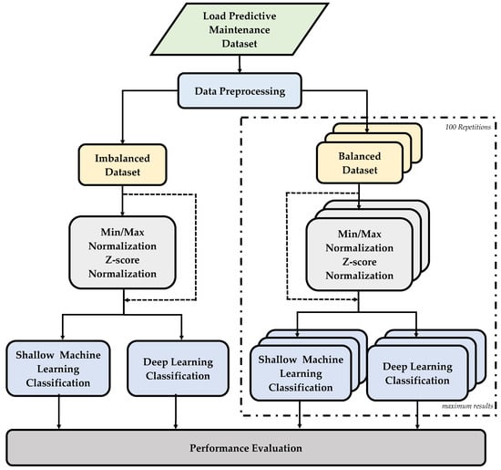
Figure 1.
Flowchart diagram of the proposed approach.
Figure 1.
Flowchart diagram of the proposed approach.
2. Materials and Methods
2.1. Dataset Description and Data Preprocessing
The dataset used for PdM known as the “AI4I 2020 Predictive Maintenance Dataset”, which is available to access in the UCI library, is utilized in this study [24]. This dataset represents actual predictive maintenance data experienced in industry, since it is hard to collect PdM statistics from production areas. Table 1 shows the features and label descriptions in the dataset. The dataset contains 10,000 cases, of which 3.4% are fault data, which makes the dataset imbalanced. Each case has six features in columns, one machine failure label and five machine failure types.

Table 1.
The description of the dataset.
Data preprocessing is the procedure of preparing data for analysis by editing, removing, or fixing data that are corrupted, incorrect, wrongly formatted, incomplete, irrelevant, or duplicated. This operation enhances data quality and helps to supply more modest, correct, and trustful data information for machine learning applications. For these reasons, the dataset was examined in the context of data preprocessing.
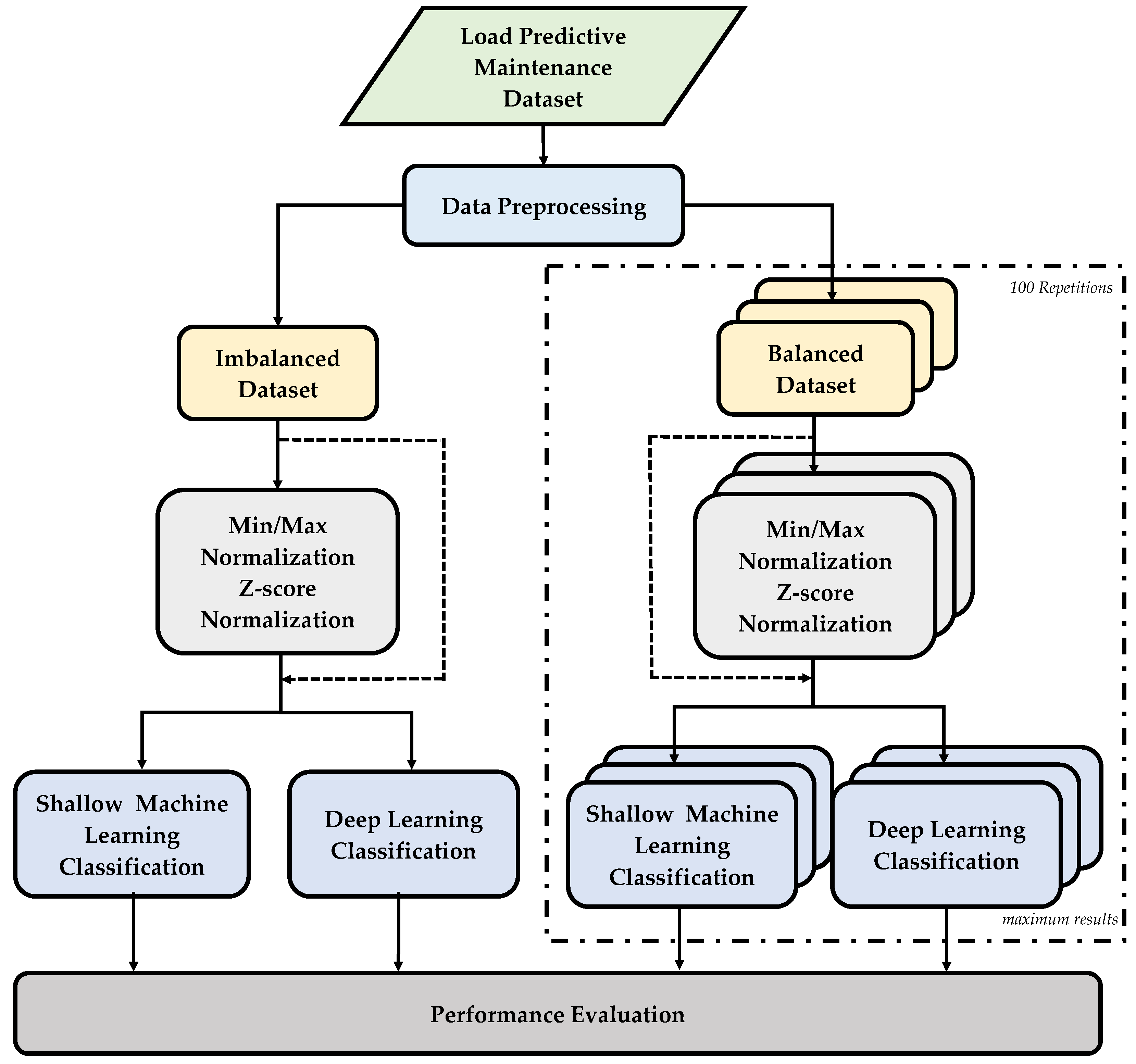
The machine failure (MF) class label is set to 1 if a machine fails and 0 otherwise. In other words, if any of the fault types from heat dissipation failure (HDF), overstrain failure (OSF), power failure (PWF), tool wear failure (TWF) occur except random failures (RNF), machine failure is reported as true. Unusual data that did not meet this condition, which is one of the contributions of this study, were excluded from the dataset. For instance, despite the fact that the RNF fault type is labeled 1 in 18 rows in the dataset, the machine failure columns are labeled as 0. Similarly, the machine failure values are labeled as 1 in 9 rows in the dataset, and the values in the fault type columns are labeled as 0. Since these rows did not contain data of any fault type and their label was machine failure 1, they were removed from the dataset. Figure 2 presents the explainable graphical structure of machine failure and non-failure classes. It illustrates the relationships among the four fault types investigated in the study—HDF, OSF, PWF, and TWF—as well as the distinct RNF fault type, in the context of both machine failure and non-failure scenarios.
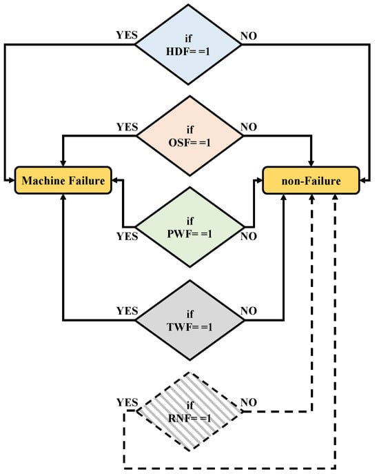
Figure 2.
The explainable graphical structure of machine failure and non-failure classes.
2.2. Feature Normalization
A normalization process is required for the data to have an equal contribution to the proposed model. The aim here is to bring the data to a common standard among the datasets so that they can be compared and to put the significant differences between the data into a single order. The most commonly used methods for data standardization are min–max normalization [26] and z-score normalization [27].
In min–max normalization [26], the original data are converted by linear conversion to the new data range, which is typically 0–1. The equation is given as follows:
where y is the normalization value, x represents the value of data, and xmin and xmax denote the minimum and maximum value of the data.
In z-score normalization, any y-value of the variable is normalized by the z-score, known as the mean and standard deviation of the variable [27]. The equations for mean, standard deviation, and z-score are as follows:
where z is the normalization value, and μ and σ denote the mean and standard deviation.
2.3. Shallow Classification Algorithms
In the classification-based machine learning approaches, classification models predict categorical labels to extract a model which represents the data classes. In our study, shallow machine learning (SML) classification algorithms are used to predict between machine failure and fault type labels from the dataset. In the following subtitles, we define the basic terms about SML algorithms such as DTs, SVMs, and k-NNs.
2.3.1. Decision Trees (DTs)
A DT is a supervised learning algorithm, which is performed for both classification and regression applications [28]. It is frequently used in machine learning due to its simple perception compared to other classification methods, lower-cost attributes, ease of integrating with a database, and high performance of reliability [29]. It is a classification method, which builds a model in the form of a tree, whose structure consists of decision nodes and leaf nodes according to classification, feature, and target. The decision tree algorithm is developed by splitting the dataset into smaller pieces. A decision node may contain one or more branches and the first node is called the root node. A decision tree can consist of both categorical and numerical data.
2.3.2. Support Vector Machines (SVMs)
Vapnik [30] created the supervised machine learning algorithm known as SVM, which is used for classification, regression, and outlier detection. Owing to its robustness and significant accuracy performance with less computational power, SVM is generally implemented for solving classification objectives. The linear SVM approach involves representing each input data point as a point in an n-dimensional space, where n corresponds to the number of input dimensions. The classification operation is performed by identifying a hyperplane that effectively separates the data into two different classes.
To provide a brief overview, SVM can be mathematically explained as follows.
In the above equation, x indicates the input feature vector of the classifier, w represents the weight vector of the hyperplane, T is the transpose, and the hyperplane position is expressed as b.
2.3.3. k-Nearest Neighbors (k-NNs)
k-NNs [31] is widely used in classification due to its simplicity, speed, flexibility in understanding and implementation, as well as its high performance and simplicity in the learning process. k-NNs determines the class of a test sample by selecting the most frequently occurring class among its k nearest neighbors. The performance of the k-NN algorithm mainly depends on the distance metric used to identify the k adjacent neighbors of a given point. Let X1 and X2 be represented by feature vectors:
where m is the dimensionality of the feature space. The adjacency can be measured by distance and the most frequently used one is the Euclidean distance given by:
where x1i and x2i are the ith features of X1 and X2, separately.
2.4. Deep Learning/CNN Architectures for Classification
In deep learning (DL), which is one of the most popular approaches in recognition and classification applications, a model can learn to perform tasks directly from data such as text, sound, or image with high accuracy achievements [32,33]. In DL models, some machine learning terms such as network design, number of layers, number of neurons, the architecture of the neural network, and optimization algorithm have gained more importance. DL uses multiple layers of nonlinear processing units for feature extraction and transformation. The most common scenario is that each node receives as inputs the outputs of every node from the previous layer in the structure [34]. Datasets used in deep learning can primarily consist of texts, images, audio, videos, or numerical data points. For instance, the image dataset consists of different features such as per-pixel density values, edge patterns, and special shapes. Some of these features better represent the original image data [35].
A convolutional neural network (CNN) is a network architecture for deep learning that learns directly from two-dimensional image input. As an end-to-end diagnostic model, it is understood from the literature that it achieves a higher performance at a lower cost [36]. A one-dimensional CNN (1D-CNN) has a less complex network structure and lower computational complexity than a two-dimensional CNN (2D-CNN) and accepts one-dimensional raw data as input directly without any preprocessing.
According to model structures and performance algorithms, one-dimensional LeNet (1D-LeNet), one-dimensional AlexNet (1D-AlexNet), and one-dimensional VGG16 (1D-VGG16) architectures are the most popular ones in 1D-CNN networks. In comparison to other types of algorithms, 1D-LeNet [37], 1D-AlexNet [38], and 1D-VGG16 [39] are used in several real engineering areas since they have simple model structures and fewer configuration parameters. In addition, 1D-LeNet, 1D-AlexNet, and 1D-VGG16 can process information more quickly and are also appropriate for fault classification. These deep learning architectures also demonstrate good performance for time series data classification [40,41].
Due to LeNet, AlexNet, and VGG16 networks having relatively simple structures and powerful classification capabilities, this paper employs these deep networks for PdM fault diagnosis. In the next section, these three types of convolutional neural network structures, called 1D-LeNet, 1D-AlexNet, and 1D-VGG16 classifiers, are presented for automatic feature extraction and fault identification of the dataset.
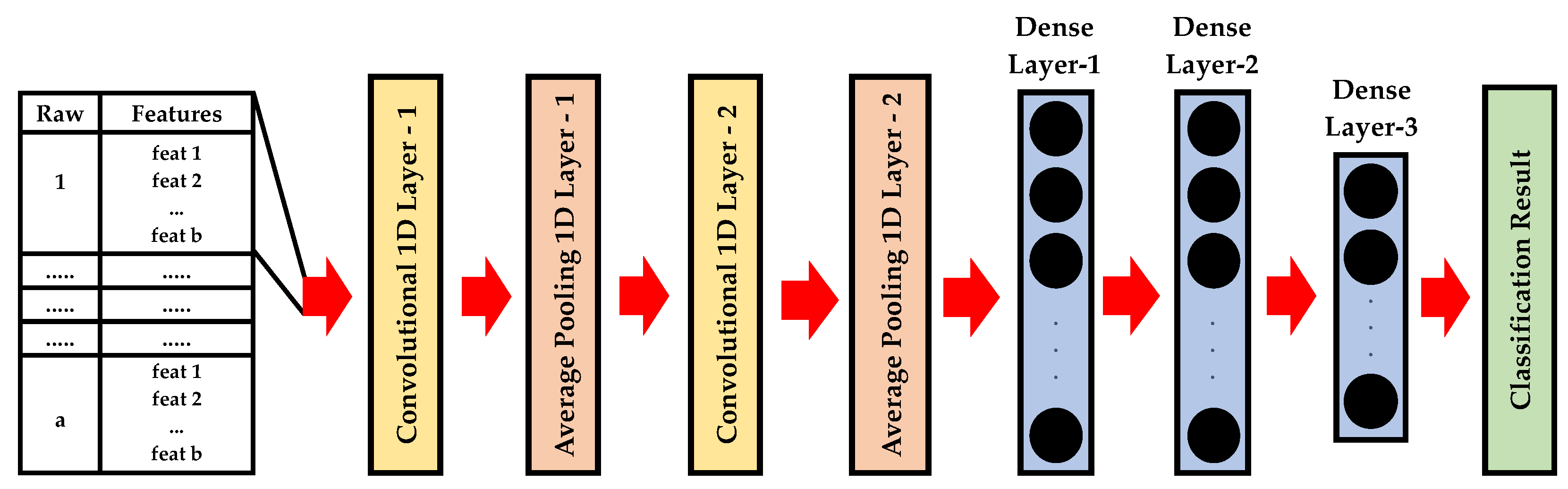
2.4.1. 1D-LeNet
The LeNet architecture, one of the convolutional neural networks, was introduced by Le Cun [37] and continued to be improved until 1998 [42]. LeNet was first proposed for digit classification, and then it was accepted to achieve promising performance in many application fields [43].
In this study, in the first instance to carry out PdM fault classification with deep learning architecture, the 1D-LeNet network is used. 1D-LeNet has two convolutional 1D layers and two average-pooling 1D layers for feature extraction, and then three fully connected layers for classification as shown in Figure 3.
Figure 3.
The structure of the 1D-LeNet.
2.4.2. 1D-AlexNet
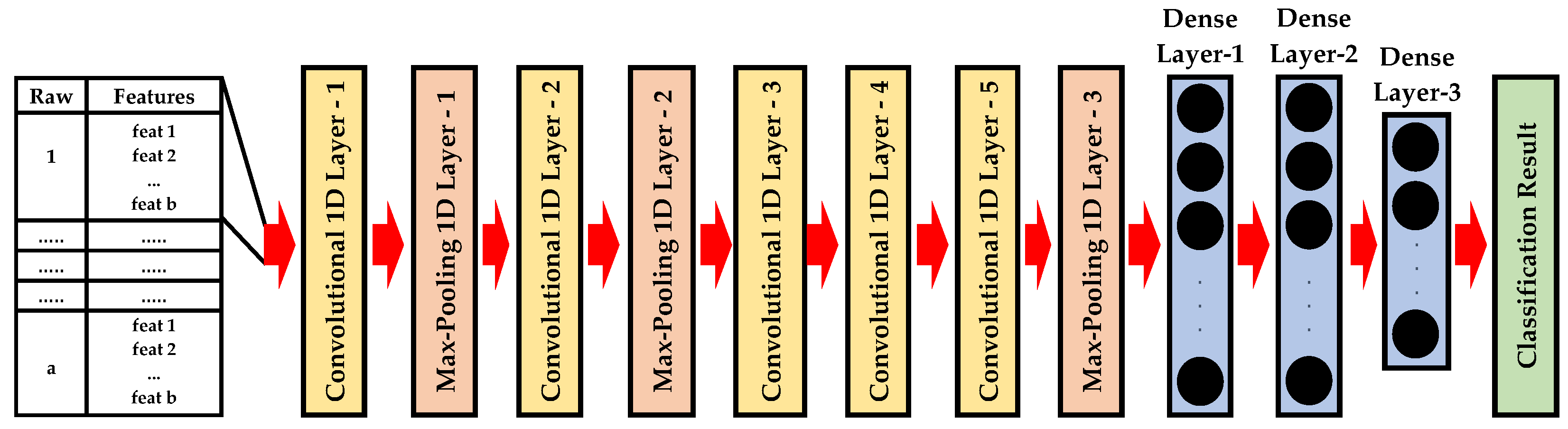
To increase accuracy and lower computing costs, epochal CNN models have been developed. One of them, AlexNet, was the lead in deep CNN models and made them popular in research on deep learning after winning the ILSVRC-2012 ImageNet competition. In this machine learning competition, the classification accuracy rate was increased from 74.3% to 83.6%, making deep learning famous again. It was developed by Alex Krizhevsky, Ilya Sutskever, and Geoffrey Hinton [38]. Convolutional neural networks are deepened by using the AlexNet structure, obtaining high accuracy in the training results. In the part of the study called PdM fault classification with deep learning, a second deep learning classifier named 1D-AlexNet architecture was used.
The 1D-AlexNet architecture has a similar design and parameters to the 1D-LeNet previously described. 1D-AlexNet has five convolutional 1D layers and three max-pooling 1D layers for feature extraction then three fully connected layers for classification. It is composed of eight layers with adjustable parameters as shown in Figure 4.
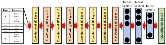
Figure 4.
The structure of 1D-AlexNet.
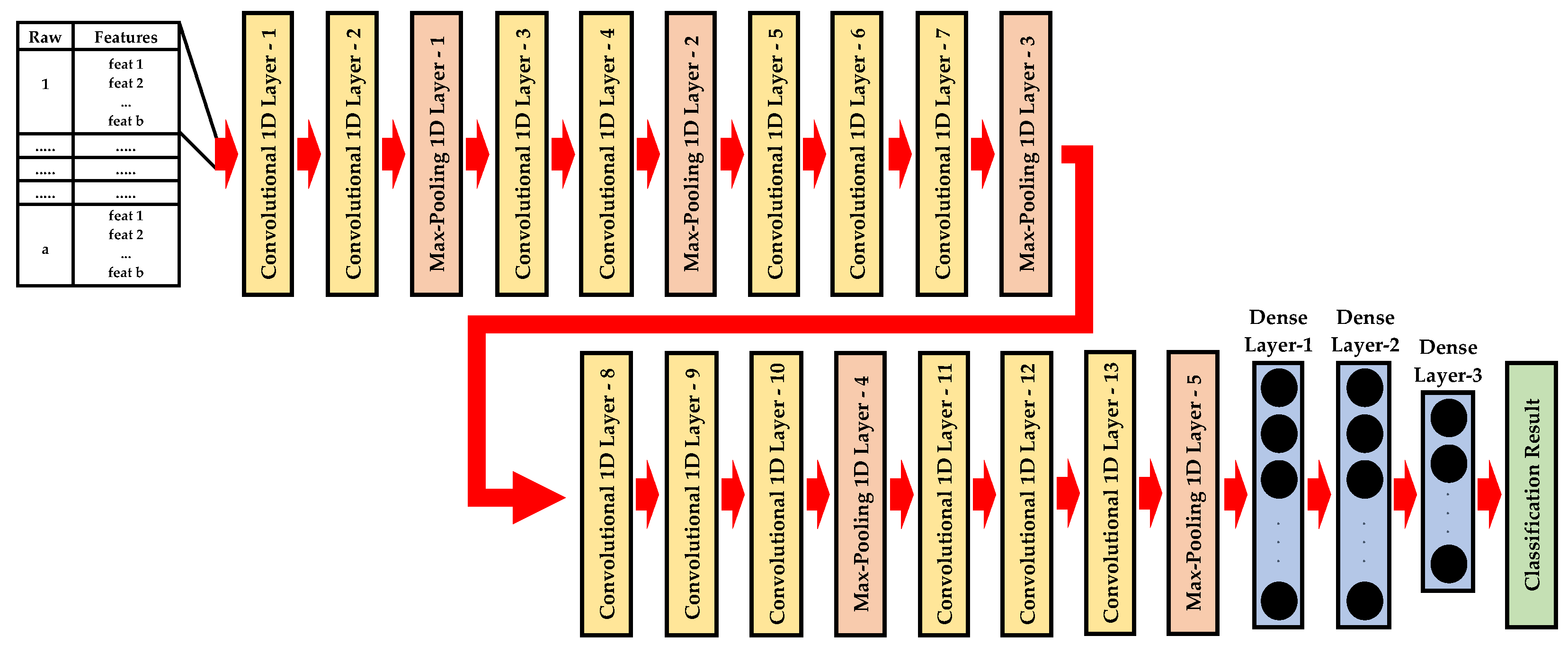
2.4.3. 1D-VGG16
The other convolutional neural network architecture known as VGG16, short for “Visual Geometry Group 16”, was created by the Visual Geometry Group at the University of Oxford [39]. The VGG-16 frame was originally designed for image classification tasks. To build another deep learning architecture for this study, the VGG16 convolutional neural network is modified for the one-dimensional PdM dataset. 1D-VGG16 mainly contains of a total of 13 convolutional 1D layers, 5 max-pooling 1D layers, and 3 fully connected layers as shown in Figure 5.
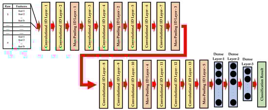
Figure 5.
The structure of 1D-VGG16.
2.5. Performance Metrics
The success of the classification model is measured by the number of samples assigned to the correct class and the number of samples assigned to the wrong class. These numbers are specified in the confusion matrix and represent how much the model is correctly predicting on the entire set of data. In a two-class example, the confusion matrix [44] is shown in Table 2.
Table 2.
The representation of the confusion matrix.
Here, TP (True Positive) denotes the determination of the positive class as a positive class. FP (False Positive) means the determination of the negative class as a positive class. TN (True Negative) represents the determination of the negative class as a negative class. FN (False Negative) refers to the determination of the positive class as a negative class. In our study, the positive class represents failure and the negative class represents non-failure.
The most popularly used performance metrics (recall, precision, specificity, accuracy, and F1-score) were used to evaluate fault classifiers in this study. The mathematical equations for each of these metrics are given in Equations (9) through (13):
In PdM fault classification applications, the performance of a classifier is calculated by its responses against unseen test input values before anything else. So, the dataset is separated into k-folds using the k-fold cross-validation (CV) method. When the k−1 portion of dataset is used for training, another is used for testing. This operation is repeated until all pieces are used for testing [45].
3. Experimental Results
The different fault types considered for this study are MF and four independent failure modes such as HDF, OSF, PWF, and TWF.
In this study, firstly, the experiments which were conducted with SML such as DTs, SVMs, and k-NNs were performed using MATLAB2021b. In continuation to our previous study, training and evaluation processes for DL classification algorithms like 1D-LeNet, 1D-AlexNet, and 1D-VGG16 were performed on a Python-based Google Colaboratory (Colab) environment utilizing NVIDIA graphics processing units (GPUs), specifically the NVIDIA-SMI version 535.104.05 with CUDA Version 12.2, and with access to 15GB of RAM.
In the all following experiments, we used 5-fold cross-validation and then 4-fold was used for training and the remaining 1-fold for testing (80% for training and 20% for testing) and we obtained the average results for the performance metrics for all fault classification studies with an imbalanced and balanced dataset with and without feature normalization.
In the Table 3 below, it is shown how the imbalanced and balanced datasets were generated as the number of rows labeled failure and non-failure for each fault types. Balanced datasets were generated 100 different times from the imbalanced data, each time ensuring the inclusion of all faulty data for each fault type, while non-failure data were randomly sampled to achieve balance each time.
Table 3.
The details of datasets used in our experiments.
3.1. Performance Metrics for MF Class Using Imbalanced Dataset without Feature Normalization
After the data preprocessing operation, the dataset is imbalanced since it comprises a total of 9973 rows which include 9643 non-failure and 330 machine-failure-labeled data. Firstly, the classification studies for the machine failure label were performed on the imbalanced dataset without any normalization.
Performance results of the classification with the imbalanced dataset without normalization are given separately in Table 4. For all experiments, the classification performance scores from different types of SML algorithms (DTs, SVMs, and k-NNs) and DL techniques (1D-LeNet, 1D-AlexNet, and 1D-VGG16) are shown in the tables. The overall accuracy values are high in both the shallow and deep machine learning algorithms.
Table 4.
Results of SML and DL classifiers for MF fault type with imbalanced and balanced dataset (without and with normalization).
When the classes are imbalanced (e.g., the majority in our dataset are in the non-failure label), the classification model performance seems good if it is evaluated according to the accuracy score. In other words, as the bias in the class distributions are high in imbalanced datasets, accuracy metrics can become unreliable [46,47]. Hence, it would be more useful to choose the F1-score (also known as F-measure), which is the most popular metric when evaluating the performance of classification in an imbalanced dataset. F1-score provides strong/reliable results for the imbalanced dataset and evaluates both the recall and precision ability of the model. According to the results that are shown in Table 4, the general F1-score values are below 54% in each shallow and deep learning classification algorithm.
In discussing other metrics, DT and SVM models demonstrate higher recall and precision compared to the other models, with DTs achieving a recall of 18.79% and precision of 87.32%, and SVM achieving a recall of 20.91% and precision of 88.46%. On the other hand, the k-NN model shows significantly higher recall (50%) but lower precision (56.70%) compared to DTs and SVMs. The 1D-LeNet, 1D-AlexNet, and 1D-VGG16 models, which are deep learning architectures, display relatively lower recall and precision values compared to DTs and SVMs. Among these, 1D-AlexNet demonstrates the highest precision at 73.68%, while 1D-LeNet has the lowest recall at 6.67%. All models show high specificity values. This is primarily based on the imbalance in the dataset, where the normal class (non-failure) overbalances the failure class. Therefore, the models tend to accurately identify the normal class (not fault class), resulting in high specificity scores.
Figure 6 shows the comparison of fault classification performance metrics for SML and DL models on an imbalanced dataset without normalization.
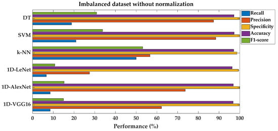
Figure 6.
Performance metrics comparison for different models on imbalanced dataset without feature normalization.
3.2. Performance Metrics for MF Class Using Balanced Dataset without Feature Normalization
In order to examine the classification performance for a balanced dataset for the machine failure label, we generated a balanced dataset which consisted of 330 rows of machine failure data and 402 rows that were randomly selected from non-failure labeled data in the dataset with 100 different repetitions. In addition to classical machine learning methods such as DTs, SVMs, and k-NNs, three types of deep learning architectures including 1D-LeNet, 1D-AlexNet, and 1D-VGG16 were utilized with 100 different balanced datasets and the maximum classification performance scores are displayed in the Table 4. The classification studies for the MF label were repeated on the balanced dataset without feature normalization.
The performance results of classification with a balanced dataset, without normalization, for both SML and DL models, were separately added to the existing Table 4. The performance metric values, especially recall, precision, and F1-score, are better, with higher results in both shallow and deep machine learning algorithms when compared to the results obtained in the previous section. It can be clearly said that improvement in these classification performance metrics for shallow machine learning algorithms is better than for deep learning architectures.
Figure 7 shows the comparison of fault classification performance metrics for SML and DL models on a balanced dataset without normalization.
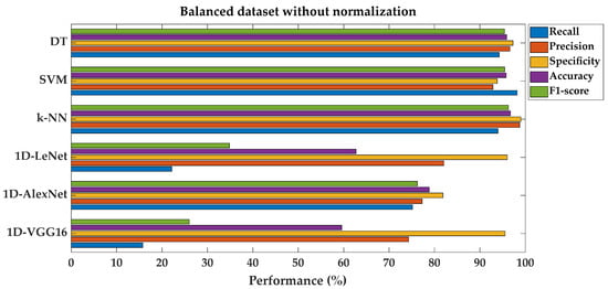
Figure 7.
Performance metrics comparison for different models on balanced dataset without feature normalization.
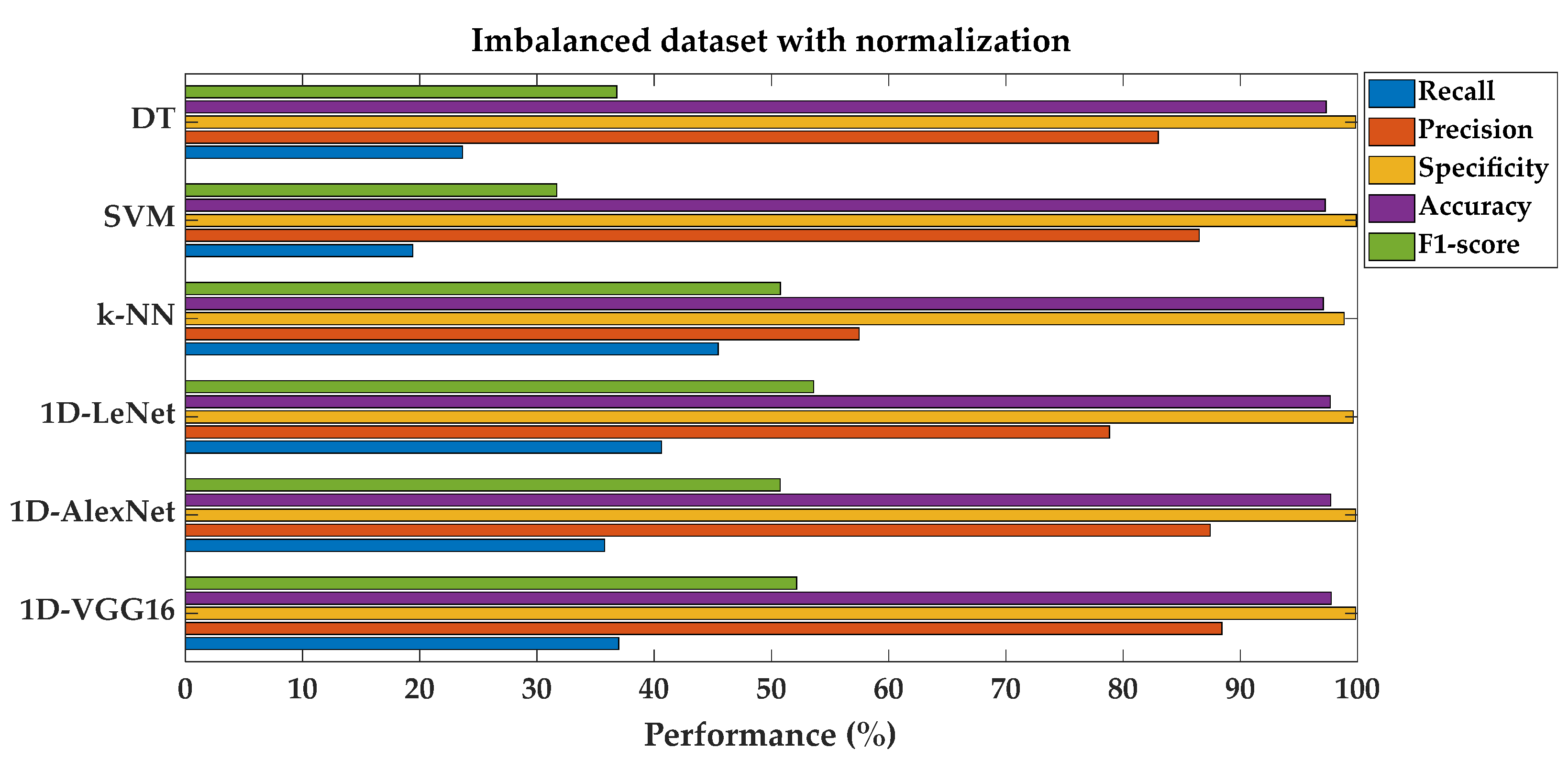
3.3. Performance Metrics for MF Class Using Imbalanced and Balanced Dataset with Feature Normalization
The normalization operation, which is one of the preprocessing techniques, was applied to ensure that all the features included in the imbalanced and balanced datasets had an equal impact on the proposed classification models.
First of all, for the machine failure label, min/max normalization and z-score normalization were performed on the features found in the imbalanced dataset and then the shallow and deep learning classification algorithms were applied on the new normalized dataset, separately. Performance metrics were calculated individually for min/max and z-score normalization. The maximum performance values of these two normalization results were added to the existing Table 4 to prevent confusion caused by an overflow of data. When analyzing the performances of the SML models, it is evident that both DT and SVM models possess higher recall and precision compared to others. Specifically, the DT model achieves a recall rate of 23.64% and a precision rate of 82.98%, while the SVM model attains a recall rate of 19.39% and a precision rate of 86.49%. Conversely, the k-NN model shows a higher recall rate of 45.45% but a lower precision rate of 57.47% when compared to DTs and SVMs. In terms of deep learning architectures, such as 1D-LeNet, 1D-AlexNet, and 1D-VGG16, they generally display relatively similar performance metrics compared to SVM models in the imbalanced dataset with feature normalization. For instance, both 1D-AlexNet and 1D-VGG16 demonstrate higher accuracy and F1-score rates at 97.70% and 50.75%, and 97.75% and 52.14%, respectively, than the SML models.
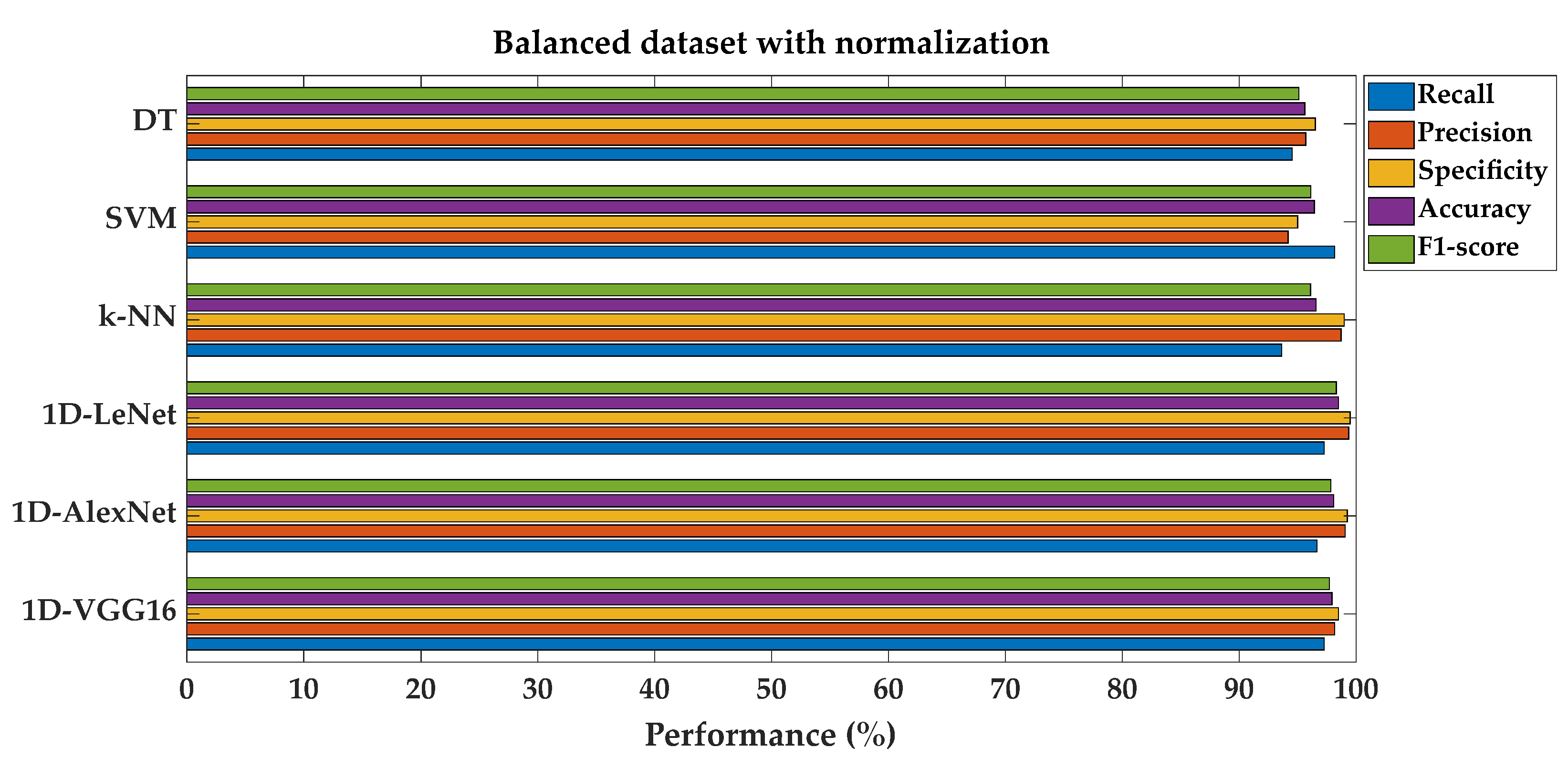
Secondly, for the MF label, the balanced dataset was generated according to Table 3. The same approach as the previous study was performed again on the balanced dataset and performance results are given separately in Table 4. After the normalization process, performance metrics in Table 4 show improvement for most of the SML algorithms and all DL architectures compared to the studies conducted in the first two sections of the experimental results. For instance, DT achieves a recall rate of 94.55% and a precision rate of 95.71% after normalization and balancing of the dataset. Similarly, SVM demonstrates a recall rate of 98.18% and a precision rate of 94.19%. Even the k-NN model, which already showed high performance, sees further improvement with a recall rate of 93.64% and a precision rate of 98.72%. Moreover, as can be seen from Table 4, the highest classification performance values were obtained in DL classification algorithms such as 1D-LeNet, 1D-AlexNet, and 1D-VGG16 using a balanced dataset with feature normalization. These models achieved remarkable recall rates of 97.27%, 96.67%, and 97.27%, respectively. Additionally, they demonstrated the highest precision rates of 99.38%, 99.07%, and 98.17%, highlighting their capacity to accurately classify fault predictions. These high recall and precision rates contributed to increased F1-scores of 98.32%, 97.85%, and 97.72%, reflecting the overall effectiveness of DL models in achieving a balance between precision and recall. Bar graphs which were prepared to visually demonstrate the performance improvement are given below. Figure 8 and Figure 9 compare fault classification performance metrics for both SML and DL models on imbalanced and balanced datasets, each with normalization.
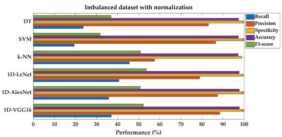
Figure 8.
Performance metrics comparison for different models on imbalanced dataset with feature normalization.
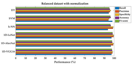
Figure 9.
Performance metrics comparison for different models on balanced dataset with feature normalization.
3.4. Performance Metrics for Fault Type Classification Using Balanced Dataset without and with Feature Normalization
In this part of the study, balanced dataset groups were generated for each fault type such as HDF, OSF, PWF, and TWF with 100 different repetitions according to Table 3. In each repetition, all failure data for each fault type and randomly selected different non-failure data are utilized in the dataset. At the conclusion of these repetitions, the maximum classification performance scores among the SML and DL classifier models were obtained for different fault types and are displayed in Table 5. The deep learning classifier models, 1D-LeNet, 1D-AlexNet, and 1D-VGG16, used for each fault type had the same structure and number of layers, neurons, and the same sizes in the fault classification experiments. Training and performance evaluation were performed by applying k-fold cross-validation and each model was trained and validated with k equal to five. SML and DL classification algorithms were separately investigated on a min/max-normalized and z-score-normalized dataset. While preparing the Table 5, the maximum performance results from two normalizations were utilized, min/max and z-score, to avoid confusion stemming from appearing data.
Table 5.
Results of SML and DL classifiers for different fault types using balanced dataset (without and with normalization).
Table 5 contains the results of experiments conducted with a balanced dataset without normalization for each fault type (HDF, OSF, PWF, and TWF), indicating that shallow classification methods achieve high values in critical performance metrics such as precision, specificity, and F1-score. In addition, as can be seen from Table 5, the one-dimensional DL models achieved higher classification performance values compared to the shallow classification models when trained on a balanced dataset with feature normalization for each fault type (HDF, OSF, PWF, and TWF). Additionally, the results demonstrate that the 1D-LeNet model achieved the highest classification performance values among all the models when trained on a balanced dataset with feature normalization for each type of fault.
4. Discussion
In the literature, many studies about fault diagnosis have been carried out with shallow classification methods. Some of these studies, which use the same dataset reflecting real PdM data [24], are presented in Table 6, along with their classification methodology, dataset type, fault type, and performance metrics.
Matzka [23] implemented an explainable model with an interface for PdM applications. A confusion matrix was generated from the results of the binary classification for the machine failure label conducted with the bagged trees ensemble classifier by applying the 5-fold cross-validation method. The accuracy and F1-score of the study were calculated as 98.34% and 77.98%, respectively. In the study, an original imbalanced dataset was used without any data preprocessing operation and without feature normalization.
The data-blind machine learning (ML) framework presented in paper [48] achieved 97.30% accuracy on the imbalanced original dataset, focusing only on the machine failure class, and used a data-blind ML algorithm without any data preprocessing, a departure from our approach outlined in this study.
Random undersampling boosting (RusBoost), GradientBoost (GB), Extreme gradient boosting (XGBoost), and Categorical Boosting (CatBoost) are boosting methods which struggle with imbalance. In studies in the literature, these models have been applied to the same dataset. Four papers using these algorithms reached 92.74% accuracy, 45.90% F1-score [49], 94.55% accuracy, 49% F1-score [50], 95.74% accuracy [51] and 88.83% accuracy [52] scores, respectively. When we compared our study with these boosting techniques, our method was found to outperform these models. For example, our paper (98.50% accuracy) demonstrated its superiority on the same predictive maintenance dataset.
In one of the other studies in the literature, the authors present a machine learning -based approach for industrial machine failure and they achieve the highest performance by using the DT classification method among the non-deep learning algorithms [53]. The selected machine learning method (DT) reached max. 77.66% F1-score values in paper. In addition to these methods, hybrid studies have used unsupervised and supervised machine learning (HUS-ML) classification algorithms. From these studies, the authors achieved the highest accuracy of 98.46% and F1-score of 78.80% [54]. Our study, including both SML and DL classification algorithms alongside data preprocessing, provides a more comprehensive analysis of not only machine failure class but also all other fault types in the dataset.
Another basic approach in fault classification involves the studies using a Random Forest (RF) model, which is one of the ensemble learning techniques [55]. The authors achieved 98.40% accuracy in their results with a dataset which was divided into two parts, such as 80% train and 20% test, without cross-validation. However, in this particular study, only shallow machine learning approaches were employed, with no cross-validation conducted. In contrast, we implemented a 5-fold cross-validation approach.
In another study in the literature [56], an approach for a mathematics-based data quality assessment of the synthetic industrial dataset [24] was proposed. They suggested a form of mathematical modeling, which is called a binary logistic regression (BLR), to be carried out for data quality evaluation verification and to solve binary classification problems. The researchers obtained the classification results as follows: accuracy was 97.10% and F1-score was 44.07%. The study was conducted with an imbalanced dataset using only machine failure class without normalization and data preprocessing.
In other studies which were implemented on the same dataset, researchers reached good performance metrics of classifiers for the prediction of machine failures with state-of-the-art methods, e.g., Density-Based Spatial Clustering of Applications with Noise (DBSCAN) and Clustering by Fast Search and Find of Density Peaks (CFSFDP—63% F1-score) [57], Evolving Fuzzy Neural Classifier with Expert rules (EFNCExp—97.30% accuracy) [58] and a Data Filling Approach based on Probability Analysis in Incomplete Soft sets (DFPAIS—83.74% accuracy) [59]. The results were directly sourced from related papers in which the authors used the same PdM dataset [24] as that used in our current study. However, unlike our study, these studies do not include data preprocessing and cleaning operations. Furthermore, our study encompasses all fault types in the original PdM dataset, enabling a performance comparison of the effects of data balancing using DL and SML.
Our study was carried out by using SML and DL classification algorithms on both an imbalanced and balanced dataset after data preprocessing operations on an original PdM dataset. In the classification performance results on the imbalanced dataset for the failure and non-failure labels, high accuracy was observed alongside relatively low F1-score values across all scores, with SML algorithms notably outperforming DL. Due to achieving higher performance on the F1-score, we employed a generation operation that involved creating 100 different balanced datasets. In each repetition, non-failure data were randomly selected to ensure a balanced representation. Subsequently, fault classification was conducted on each dataset, with the maximum results recorded from these iterations. Since the ranges of features are very different in the used dataset, feature normalization methods such as min–max normalization and z-score normalization were applied. It was observed that feature normalization moderately increased the performance of the classification performance metrics in SML and especially DL classification methods. In this paper, considering the machine learning-based approaches, it can be said that classification performance results obtained from balanced datasets have higher overall performance values than imbalanced ones. To summarize, it is seen from Table 6 that 1D-LeNet, 1D-AlexNet, and 1D-VGG16 algorithms from DL classifiers reached better performance results compared to SML approaches such as DTs, SVMs, and k-NNs in this study.
Table 6.
Performance comparison using classification algorithms with same dataset.
Table 6.
Performance comparison using classification algorithms with same dataset.
| Literature | Classification Algorithm | Dataset Type | Fault Class | Performance Metrics (%) | |
|---|---|---|---|---|---|
| Matzka [23] | Bagged Trees | Imbalanced | MF | Acc = 98.34 | F1 = 77.98 |
| Pastorino and Biswas [48] | Data-Blind Machine Learning | Imbalanced | MF | Acc = 97.30 | F1 = - |
| Torcianti and Matzka [49] | Random Undersampling Boosting Trees | Imbalanced | MF | Acc = 92.74 | F1 = 45.90 |
| Diao et al. [57] | Density-Based Spatial Clustering of Applications with NoiseClustering by Fast Search and Find of Density Peaks | Imbalanced | MF | Acc = - | F1 = 63.00 |
| Mota et al. [50] | Gradient Boosting | Imbalanced | MF | Acc = 94.55 | F1 = 49.00 |
| Vuttipittayamongkol and Arreeras [53] | Decision Tree | Imbalanced | MF | Acc = - | F1 = 77.66 |
| de Campos Souza and Lughofer [58] | Evolving Fuzzy Neural Classifier with Expert rules | Imbalanced | MF | Acc = 97.30 | F1 = - |
| Sharma et al. [55] | Random Forest | Imbalanced | MF | Acc = 98.40 | F1 = - |
| Iantovics and Enăchescu [56] | Binary Logistic Regression | Imbalanced | MF | Acc = 97.10 | F1 = 44.07 |
| Vandereycken and Voorhaar [51] | Extreme Gradient Boosting | Imbalanced | MF | Acc = 95.74 | F1 = - |
| Chen et al. [52] | Combination of Synthetic minority oversampling technique for nominal and continuous, Conditional tabular generative adversarial network and Categorical Boosting | Imbalanced | MF | Acc = 88.83 | F1 = - |
| Harichandran et al. [54] | Hybrid Unsupervised and Supervised Machine Learning | Imbalanced | MF | Acc = 98.46 | F1 = 78.80 |
| Kong et al. [59] | A Data Filling Approach based on Probability Analysis in Incomplete Soft sets | Imbalanced | MF | Acc = 83.74 | F1 = - |
| In this study | Decision Trees | Imbalanced | MF | Acc = 97.31 | F1 = 36.79 |
| Support Vector Machines | Imbalanced | MF | Acc = 97.29 | F1 = 33.82 | |
| k-Nearest Neighbors | Imbalanced | MF | Acc = 97.08 | F1 = 53.14 | |
| 1D-LeNet | Balanced | MF | Acc = 98.50 | F1 = 98.32 | |
| 1D-AlexNet | Balanced | MF | Acc = 98.09 | F1 = 97.85 | |
| 1D-VGG16 | Balanced | MF | Acc = 97.95 | F1 = 97.72 | |
MF: machine failure, Acc: accuracy, and F1: F1-score.
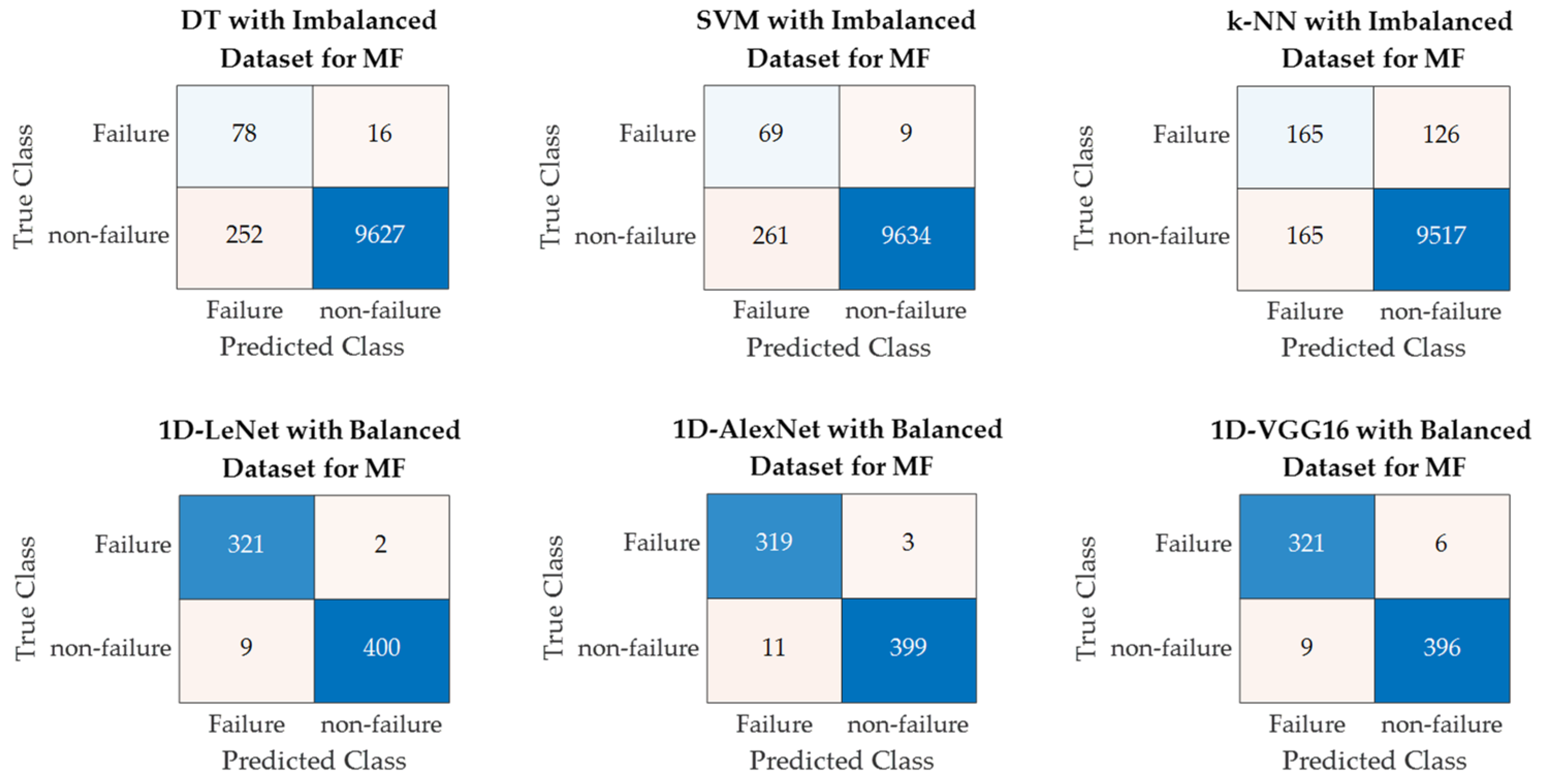
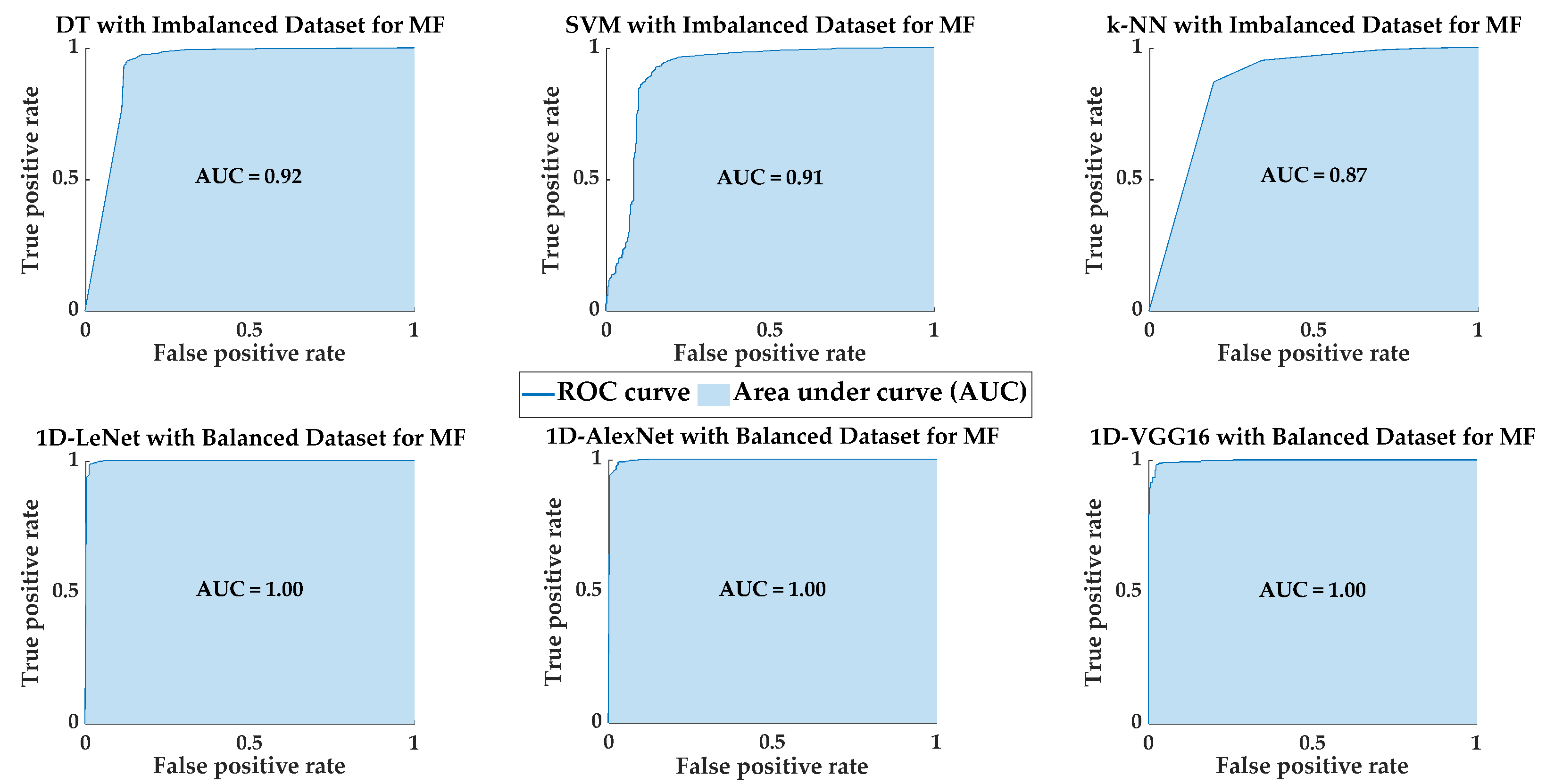
Figure 10 shows the confusion matrices for PdM fault classification using SML and DL models, illustrating the highest classification performance achieved by each model. Additionally, Figure 11 presents the ROC curves and AUC values for SML and DL models, demonstrating the highest classification performance achieved by each model. In future studies, we will apply data augmentation techniques to the original PdM dataset. In addition to binary classification, multi-class classification will be conducted to classify different fault types present in the original PdM dataset, and their performance will be examined. Also, in future studies, one-dimensional predictive maintenance data will be transformed into two-dimensional images and fault classification will be performed on these images using different deep learning algorithms.
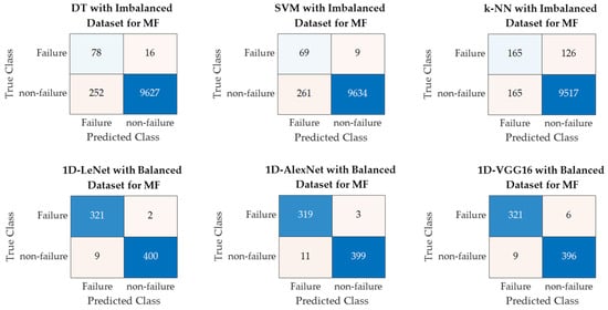
Figure 10.
Confusion matrices for fault classification using SML algorithms and 1-D DL models.
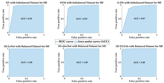
Figure 11.
The ROC curve and AUC values for fault classification using SML algorithms and 1D DL models.
5. Conclusions
In this study, we examined the machine learning techniques for detecting and classifying the failures in a dataset which structurally reflects real predictive maintenance sensor data commonly encountered in industry. DL architectures such as LeNet, AlexNet, and VGG16 models in their one-dimensional versions achieved much better classification performances than SML methods on balanced datasets. Additionally, we generated 100 different balanced datasets from the imbalanced dataset. Separate simulations were conducted for each dataset, and the maximum performance results are presented in the tables. The classification methods proposed in the study reached successful high performance values, even though different dataset groups and fault types from the original PdM dataset were used in comparison to other studies in the literature. From the experimental results and discussion, it can be surely said that when data balance is achieved, using 1D-LeNet deep learning classifiers and feature normalization processes enhances the capability of recognizing and categorizing the faults with a highest accuracy and F1-score of 98.50% and 98.32%, respectively. Especially, the F1-score demonstrates a 20% improvement compared to the highest F1-score from studies in the literature. When considering all the results obtained in the study collectively, one-dimensional deep learning classification methods on a balanced dataset with normalized features can be recommended for the practical applications of fault classification in the PdM studies.
Author Contributions
Software, U.I., Y.A. and A.N.; methodology, U.I., Y.A. and A.N.; writing—original draft, U.I.; writing—review and editing, U.I., Y.A. and A.N.; supervision, Y.A. and A.N. All authors have read and agreed to the published version of the manuscript.
Funding
This research received no external funding.
Institutional Review Board Statement
Not applicable.
Informed Consent Statement
Not applicable.
Data Availability Statement
We used a publicly available dataset called the “AI4I 2020 Predictive Maintenance” for our study, from the UCI data repository [24].
Conflicts of Interest
The authors declare no conflicts of interest.
References
- Vermesan, O.; Friess, P. (Eds.) Internet of Things: Converging Technologies for Smart Environments and Integrated Ecosystems; River Publishers: Aalborg, Denmark, 2013. [Google Scholar]
- Guzmán, V.E.; Muschard, B.; Gerolamo, M.; Kohl, H.; Rozenfeld, H. Characteristics and Skills of Leadership in the Context of Industry 4.0. Procedia Manuf. 2020, 43, 543–550. [Google Scholar] [CrossRef]
- Cao, Q.; Zanni-Merk, C.; Samet, A.; Reich, C.; De Beuvron, F.D.B.; Beckmann, A.; Giannetti, C. KSPMI: A knowledge-based system for predictive maintenance in industry 4.0. Robot. Comput. Integr. Manuf. 2022, 74, 102281. [Google Scholar] [CrossRef]
- Li, Z. Deep Learning Driven Approaches for Predictive Maintenance: A Framework of Intelligent Fault Diagnosis and Prognosis in the Industry 4.0 Era. Ph.D. Thesis, Norwegian University of Science and Technology, Trondheim, Norway, 2018; p. 132. [Google Scholar]
- Levitt, J. Complete Guide to Preventive and Predictive Maintenance; Industrial Press Inc.: South Norwalk, CT, USA, 2003. [Google Scholar]
- Achouch, M.; Dimitrova, M.; Dhouib, R.; Ibrahim, H.; Adda, M.; Sattarpanah Karganroudi, S.; Ziane, K.; Aminzadeh, A. Predictive Maintenance and Fault Monitoring Enabled by Machine Learning: Experimental Analysis of a TA-48 Multistage Centrifugal Plant Compressor. Appl. Sci. 2023, 13, 1790. [Google Scholar] [CrossRef]
- Velmurugan, R.S.; Dhingra, T. Maintenance strategy selection and its impact in maintenance function: A conceptual framework. Int. J. Oper. Prod. Manag. 2015, 35, 1622–1661. [Google Scholar] [CrossRef]
- Kiangala, K.S.; Wang, Z. Initiating predictive maintenance for a conveyor motor in a bottling plant using industry 4.0 concepts. Int. J. Adv. Manuf. Technol. 2018, 97, 3251–3271. [Google Scholar] [CrossRef]
- Lee, J. Machine performance monitoring and proactive maintenance in computer-integrated manufacturing: Review and perspective. Int. J. Comput. Integr. Manuf. 1995, 8, 370–380. [Google Scholar] [CrossRef]
- Li, D.; Landström, A.; Fast-Berglund, Å.; Almström, P. Human-centred dissemination of data, information and knowledge in industry 4.0. Procedia CIRP 2019, 84, 380–386. [Google Scholar] [CrossRef]
- Baccarini, L.M.R.; e Silva, V.V.R.; de Menezes, B.R.; Caminhas, W.M. SVM practical industrial application for mechanical faults diagnostic. Expert Syst. Appl. 2011, 38, 6980–6984. [Google Scholar] [CrossRef]
- Zhang, Z.; Wang, Y.; Wang, K. Fault diagnosis and prognosis using wavelet packet decomposition, Fourier transform and artificial neural network. J. Intell. Manuf. 2013, 24, 1213–1227. [Google Scholar] [CrossRef]
- Xiong, G.; Shi, D.; Chen, J.; Zhu, L.; Duan, X. Divisional fault diagnosis of large-scale power systems based on radial basis function neural network and fuzzy integral. Electr. Power Syst. Res. 2013, 105, 9–19. [Google Scholar] [CrossRef]
- Muralidharan, V.; Sugumaran, V. Feature extraction using wavelets and classification through decision tree algorithm for fault diagnosis of mono-block centrifugal pump. Measurement 2013, 46, 353–359. [Google Scholar] [CrossRef]
- Phillips, J.; Cripps, E.; Lau, J.W.; Hodkiewicz, M.R. Classifying machinery condition using oil samples and binary logistic regression. Mech. Syst. Signal Process. 2015, 60, 316–325. [Google Scholar] [CrossRef]
- Konar, P.; Chattopadhyay, P. Bearing fault detection of induction motor using wavelet and Support Vector Machines (SVMs). Appl. Soft Comput. 2011, 11, 4203–4211. [Google Scholar] [CrossRef]
- Rai, A.; Upadhyay, S.H. Intelligent bearing performance degradation assessment and remaining useful life prediction based on self-organising map and support vector regression. Proc. Inst. Mech. Eng. Part C J. Mech. Eng. Sci. 2018, 232, 1118–1132. [Google Scholar] [CrossRef]
- Orrù, P.F.; Zoccheddu, A.; Sassu, L.; Mattia, C.; Cozza, R.; Arena, S. Machine Learning Approach Using MLP and SVM Algorithms for the Fault Prediction of a Centrifugal Pump in the Oil and Gas Industry. Sustainability 2020, 12, 4776. [Google Scholar] [CrossRef]
- Pinedo-Sanchez, L.A.; Mercado-Ravell, D.A.; Carballo-Monsivais, C.A. Vibration analysis in bearings for failure prevention using CNN. J. Braz. Soc. Mech. Sci. Eng. 2020, 42, 628. [Google Scholar] [CrossRef]
- Deng, H.; Zhang, W.X.; Liang, Z.F. Application of BP Neural Network and Convolutional Neural Network (CNN) in Bearing Fault Diagnosis. Mater. Sci. Eng. 2021, 1043, 42–46. [Google Scholar] [CrossRef]
- Gao, J.; Han, H.; Ren, Z.; Fan, Y. Fault diagnosis for building chillers based on data self-production and deep convolutional neural network. J. Build. Eng. 2021, 34, 102043. [Google Scholar] [CrossRef]
- Zheng, J.; Liu, Y.; Ge, Z. Dynamic Ensemble Selection Based Improved Random Forests for Fault Classification in Industrial Processes. IFAC J. Syst. Control 2022, 20, 100189. [Google Scholar] [CrossRef]
- Matzka, S. Explainable artificial intelligence for predictive maintenance applications. In Proceedings of the Third International Conference on Artificial Intelligence for Industries, Irvine, CA, USA, 21–23 September 2020; pp. 69–74. [Google Scholar]
- Matzka, S. AI4I 2020 Predictive Maintenance Dataset. UCI Machine Learning Repository. 2020. Available online: www.explorate.ai/dataset/predictiveMaintenanceDataset.csv (accessed on 22 December 2021).
- Azeri, N.; Hioual, O.; Hioual, O. Towards an Approach for Modeling and Architecting of Self-Adaptive Cyber-Physical Systems. In Proceedings of the 2022 4th International Conference on Pattern Analysis and Intelligent Systems (PAIS), Oum El Bouaghi, Algeria, 12–13 October 2022; pp. 1–7. [Google Scholar]
- Han, J.; Kamber, M.; Pei, J. Data Mining: Concepts and Techniques, 3rd ed.; Morgan Kaufmann Publisher: Waltham, MA, USA, 2011. [Google Scholar]
- Bhanja, S.; Das, A. Impact of Data Normalization on Deep Neural Network for Time Series Forecasting. arXiv 2018, arXiv:1812.05519. [Google Scholar]
- Quinlan, J.R. C4. 5: Programs for Machine Learning; Elsevier: Amsterdam, The Netherlands, 2014. [Google Scholar]
- Chien, C.F.; Chen, L.F. Data mining to improve personnel selection and enhance human capital: A case study in high-technology industry. Expert Syst. Appl. 2008, 34, 280–290. [Google Scholar] [CrossRef]
- Vapnik, V.N. An overview of statistical learning theory. IEEE Trans. Neural Netw. 1999, 10, 988–999. [Google Scholar] [CrossRef] [PubMed]
- Cover, T.; Hart, P. Nearest Neighbor pattern classification. IEEE Trans. Inf. Theory 1967, 13, 21–27. [Google Scholar] [CrossRef]
- Kim, S.H.; Choi, H.L. Convolutional Neural Network for Monocular Vision-based Multi-target Tracking. Int. J. Control Autom. Syst. 2019, 17, 2284–2296. [Google Scholar] [CrossRef]
- Lee, S.J.; Choi, H.; Hwang, S.S. Real-time Depth Estimation Using Recurrent CNN with Sparse Depth Cues for SLAM System. Int. J. Control Autom. Syst. 2020, 18, 206–216. [Google Scholar] [CrossRef]
- Deng, L. Deep Learning: Methods and Applications. Found. Trends Signal Process. 2013, 7, 197–387. [Google Scholar] [CrossRef]
- Song, H.A.; Lee, S.Y. Hierarchical Representation Using NMF. In International Conference on Neural Information Processing; Springer: Berlin/Heidelberg, Germany, 2013. [Google Scholar]
- Abdeljaber, O.; Sassi, S.; Avci, O.; Kiranyaz, S.; Ibrahim, A.A.; Gabbouj, M. Fault detection and severity identification of ball bearings by online condition monitoring. IEEE Trans. Ind. Electro 2018, 66, 8136–8147. [Google Scholar] [CrossRef]
- Le Cun, Y.; Jackel, L.D.; Boser, B.; Denker, J.S.; Graf, H.P.; Guyon, I.; Henderson, D.; Howard, R.E.; Hubbard, W. Handwritten digit recognition: Applications of neural network chips and automatic learning. IEEE Commun. Mag. 1989, 27, 41–46. [Google Scholar] [CrossRef]
- Krizhevsky, A.; Sutskever, I.; Hinton, G.E. Imagenet classification with deep convolutional neural networks. Commun. ACM 2017, 60, 84–90. [Google Scholar] [CrossRef]
- Simonyan, K.; Zisserman, A. Very deep convolutional networks for large-scale image recognition. arXiv 2014, arXiv:1409.1556. [Google Scholar]
- Wu, Y.; Yang, F.; Liu, Y.; Zha, X.; Yuan, S. A comparison of 1-D and 2-D deep convolutional neural networks in ECG classification. arXiv 2018, arXiv:1810.07088. [Google Scholar]
- Xie, S.; Ren, G.; Zhu, J. Application of a new one-dimensional deep convolutional neural network for intelligent fault diagnosis of rolling bearings. Sci. Prog. 2020, 103, 36850420951394. [Google Scholar] [CrossRef]
- Lecun, Y.; Bottou, L.; Bengio, Y.; Haffner, P. Gradient-based learning applied to document recognition. Proc. IEEE 1998, 86, 2278–2324. [Google Scholar] [CrossRef]
- Eren, L. Bearing fault detection by one-dimensional convolutional neural networks. Math. Probl. Eng. 2017, 2017, 8617315. [Google Scholar] [CrossRef]
- Pietikäinen, M. Local Binary Patterns. Scholarpedia 2010, 5, 9775. [Google Scholar] [CrossRef]
- Rodriguez, J.D.; Perez, A.; Lozano, J.A. Sensitivity Analysis of k-Fold Cross Validation in Prediction Error Estimation. IEEE Trans. Pattern Anal. Mach. Intell. 2010, 32, 569–575. [Google Scholar] [CrossRef]
- Batista, G.E.; Prati, R.C.; Monard, M.C. A study of the behavior of several methods for balancing machine learning training data. ACM SIGKDD Explor. Newsl. 2004, 6, 20–29. [Google Scholar] [CrossRef]
- Hossin, M.; Sulaiman, M. A review on evaluation metrics for data classification evaluations. Int. J. Data Min. Knowl. Manag. Process 2015, 5, 1. [Google Scholar]
- Pastorino, J.; Biswas, A.K. Data-Blind ML: Building privacy-aware machine learning models without direct data access. In Proceedings of the IEEE Fourth International Conference on Artificial Intelligence and Knowledge Engineering, Laguna Hills, CA, USA, 1–3 December 2021; pp. 95–98. [Google Scholar]
- Torcianti, A.; Matzka, S. Explainable Artificial Intelligence for Predictive Maintenance Applications using a Local Surrogate Model. In Proceedings of the 4th International Conference on Artificial Intelligence for Industries, Laguna Hills, CA, USA, 20–22 September 2021; pp. 86–88. [Google Scholar]
- Mota, B.; Faria, P.; Ramos, C. Predictive Maintenance for Maintenance-Effective Manufacturing Using Machine Learning Approaches. In Proceedings of the 17th International Conference on Soft Computing Models in Industrial and Environmental Applications, Salamanca, Spain, 5–7 September 2022; Lecture Notes in Networks and Systems. Volume 531, pp. 13–22. [Google Scholar]
- Vandereycken, B.; Voorhaar, R. TTML: Tensor trains for general supervised machine learning. arXiv 2022, arXiv:2203.04352. [Google Scholar]
- Chen, C.-H.; Tsung, C.-K.; Yu, S.-S. Designing a Hybrid Equipment-Failure Diagnosis Mechanism under Mixed-Type Data with Limited Failure Samples. Appl. Sci. 2022, 12, 9286. [Google Scholar] [CrossRef]
- Vuttipittayamongkol, P.; Arreeras, T. Data-driven Industrial Machine Failure Detection in Imbalanced Environments. In Proceedings of the IEEE International Conference on Industrial Engineering and Engineering Management, Kuala Lumpur, Malaysia, 7–10 December 2022; pp. 1224–1227. [Google Scholar]
- Harichandran, A.; Raphael, B.; Mukherjee, A. Equipment Activity Recognition and Early Fault Detection in Automated Construction through a Hybrid Machine Learning Framework. Comput. Aided Civ. Infrastruct. Eng. 2022, 38, 253–268. [Google Scholar] [CrossRef]
- Sharma, N.; Sidana, T.; Singhal, S.; Jindal, S. Predictive Maintenance: Comparative Study of Machine Learning Algorithms for Fault Diagnosis. In Proceedings of the Proceedings of the International Conference on Innovative Computing & Communication (ICICC), Delhi, India, 19–20 February 2022. [Google Scholar]
- Iantovics, L.B.; Enăchescu, C. Method for Data Quality Assessment of Synthetic Industrial Data. Sensors 2022, 22, 1608. [Google Scholar] [CrossRef] [PubMed]
- Diao, L.; Deng, M.; Gao, J. Clustering by Constructing Hyper-Planes. IEEE Access 2021, 9, 70167–70181. [Google Scholar] [CrossRef]
- Souza, P.V.C.; Lughofer, E. EFNC-Exp: An evolving fuzzy neural classifier integrating expert rules and uncertainty. Fuzzy Sets Syst. 2023, 466, 108438. [Google Scholar] [CrossRef]
- Kong, Z.; Lu, Q.; Wang, L.; Guo, G. A Simplified Approach for Data Filling in Incomplete Soft Sets. Expert Syst. Appl. 2023, 213, 119248. [Google Scholar] [CrossRef]


Disclaimer/Publisher’s Note: The statements, opinions and data contained in all publications are solely those of the individual author(s) and contributor(s) and not of MDPI and/or the editor(s). MDPI and/or the editor(s) disclaim responsibility for any injury to people or property resulting from any ideas, methods, instructions or products referred to in the content. |
© 2024 by the authors. Licensee MDPI, Basel, Switzerland. This article is an open access article distributed under the terms and conditions of the Creative Commons Attribution (CC BY) license (https://creativecommons.org/licenses/by/4.0/).