
Text Classification Model Based on Graph Attention Networks and Adversarial Training

Abstract
Featured Application
Abstract
1. Introduction
- We utilize three distinct graph attention networks (GATs) to extract features from the contextual vocabulary of input text sequences. By concatenating these features with the original input text sequences, we achieve a superior representation of the text.
- During the model training process, we introduce noise perturbations for adversarial training. Experimental results indicate that the incorporation of noise perturbations enhances the model’s generalization ability on original samples and improves robustness.
- We employ a multi-head attention mechanism, wherein the weight matrices assign higher numerical values to key information. The experiments demonstrate that this approach can further enhance classification accuracy.
2. Materials and Methods
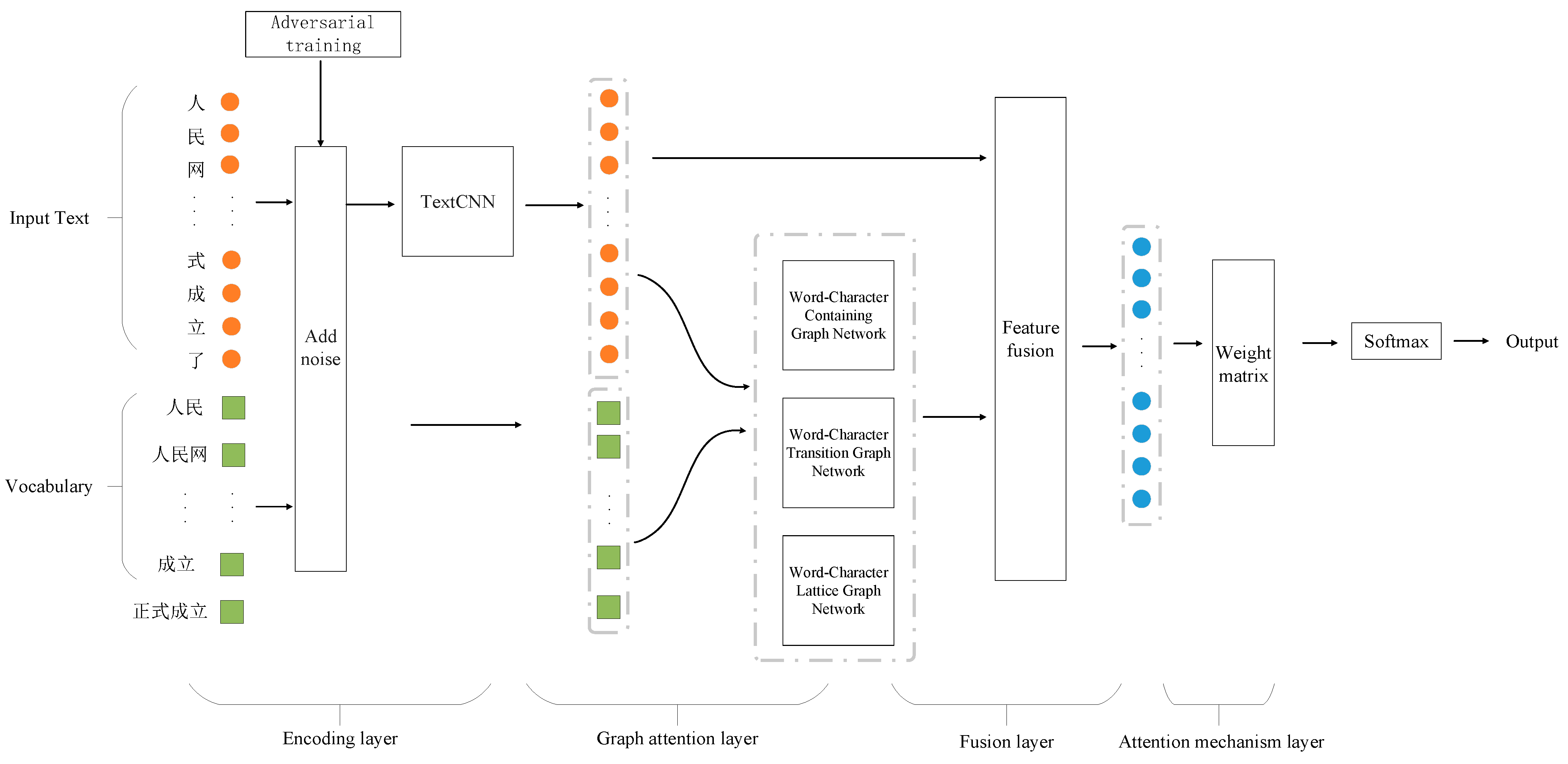
2.1. Model Framework
2.1.1. Subsection Encoding Layer
2.1.2. Graph Attention Layer
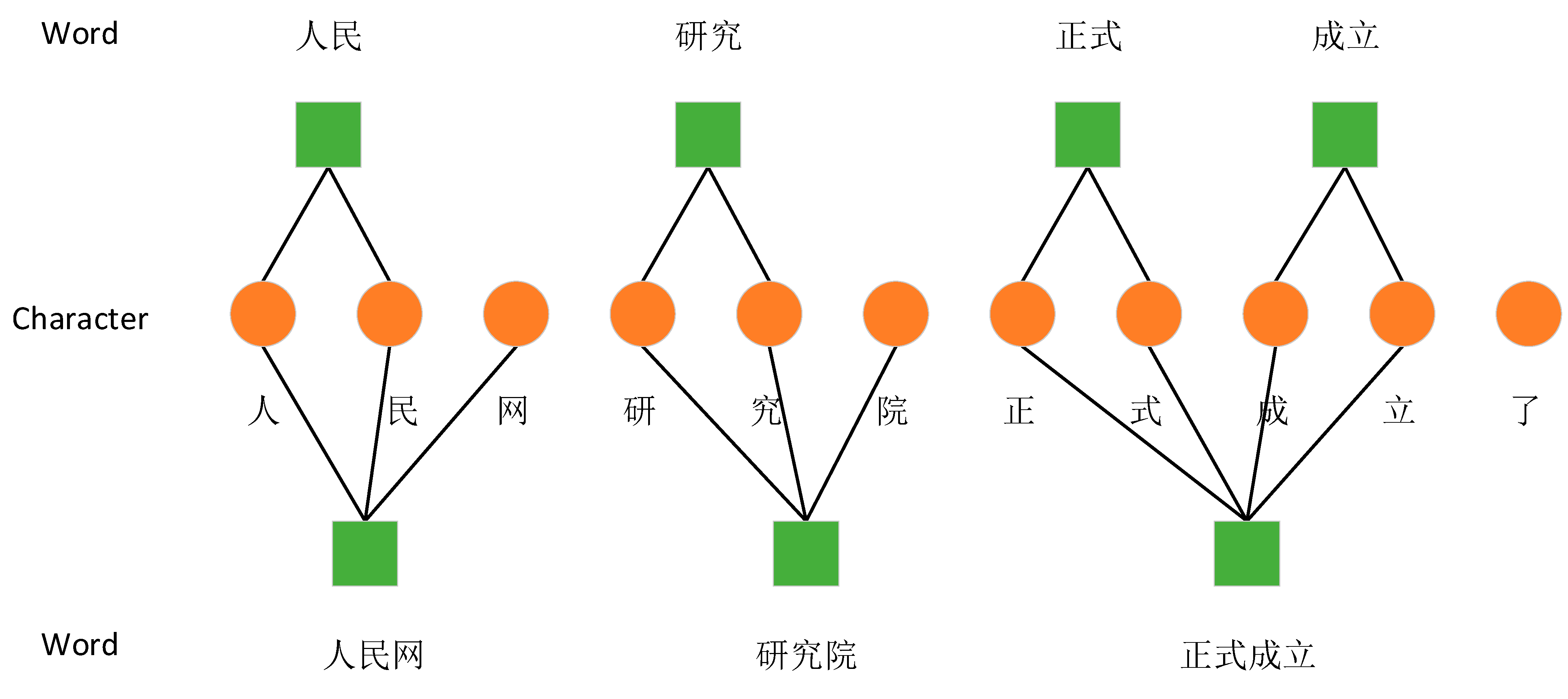
- Word–Character Containing Graph Network: This network is designed to aid characters in acquiring boundary information and semantic information from self-matching vocabulary. It establishes connections between characters and their directly associated words, enriching the characters with deeper lexical insights.
- Word–Character Transition Graph Network: This network captures the semantic information of the nearest contextual vocabulary. It transitions between characters and words that form contextual relationships, helping to understand the flow and connection of ideas within the text.
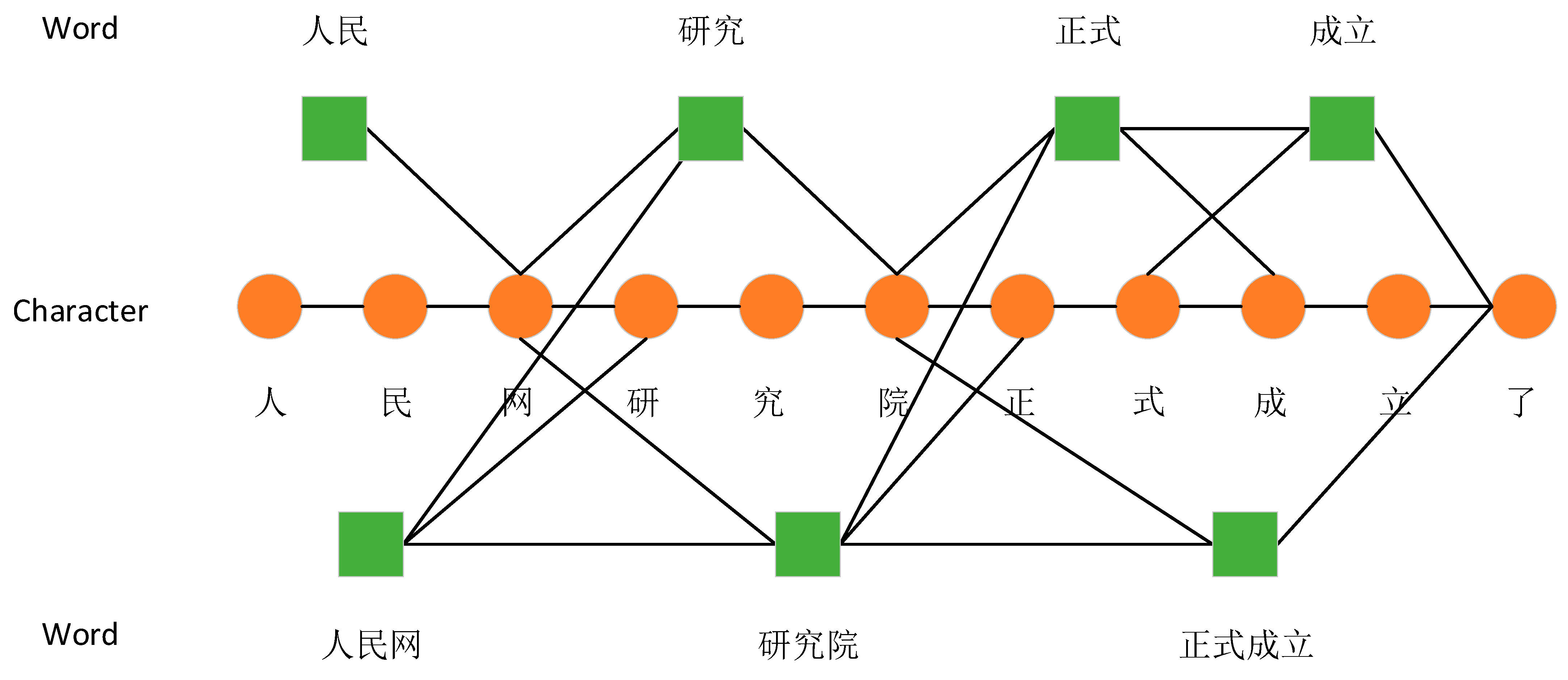
- Word–Character Lattice Graph Network: Inspired by Zhang Yue’s [23] use of a lattice structure in LSTM models to integrate vocabulary knowledge, this paper extracts the lattice structure to form the third attention network layer. This structure allows for a more flexible and interconnected approach to handling complex character–word relationships, providing a mesh-like framework that captures broader lexical fields.
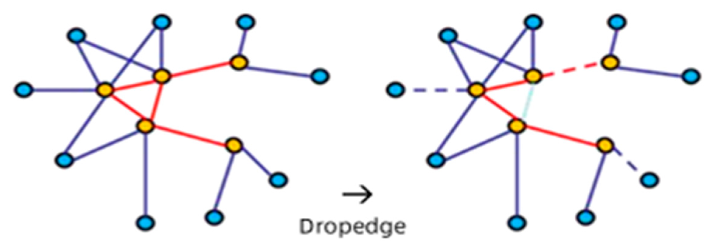
2.1.3. Adjacency Matrix Processing
2.1.4. Fusion Layer
2.1.5. Attention Mechanism Layer
2.2. Experiments
2.2.1. Data Collection and Preprocessing
2.2.2. Hardware Configuration
2.2.3. Parameter Settings
2.2.4. Comparison Model
- TextCNN [7]: This utilizes Word2Vec to generate word vectors, followed by feature extraction through convolutional kernels of varying sizes. After passing through a max pooling layer, classification is performed using a Softmax function.
- TextCNN+Att: After feature extraction using convolutional kernels of different sizes, the text passes through a weight adjustment layer that uses an attention mechanism to adjust weight values. This layer captures the dependency relationships between words based on the degree of influence of each word in the sequence on the text classification task and can learn the internal structural information of the sequence text.
- TextRNN [8]: The use of RNN can effectively process sequence information and better extract contextual information features.
- Transformer [28]: This comprises an encoder and decoder, using Word2Vec for converting input text into feature vectors. The self-attention mechanism effectively addresses the problem of long-distance dependencies in classification tasks.
- BiLSTM [8]: This generates word vectors using Word2Vec and utilizes bidirectional LSTM layers to extract semantic information and dependencies in text, followed by classification through a fully connected layer.
- HANs [29]: HANs is a Chinese short text classification model that uses CNN and BiLSTM to encode the character level and word-level features, respectively, and concatenates two-level features for classification.
- CNN-highway + RNN [1]: This is a Chinese text classification model based on character-level features, where the sentence is encoded by highway-CNN and LSTM, respectively, and two outputs are concatenated for classification.
- TextGCN [14]: Text-GCN constructs a heterogeneous graph based on the document and its words, and enables graph convolution networks to perform semi-supervised text classification.
- Text-level-GNN [30]: Text-level-GNN is a text-level graph neural network model-based message passing mechanism, where a graph is constructed for each sentence and the words in the sentence are viewed as nodes.
- RAFG [31]: RAFG is a Chinese text classification model that uses BiLSTMs to encode the Chinese radical information at character-level and word-level, respectively.
- MACNN [32]: MACNN is a Chinese short text classification model to integrate character-level and word-level features by sentence-level attention mechanisms.
- CW-GAT [33]: CW-GAT is a model that utilizes graph attention networks to effectively capture and integrate the interaction between character-level and word-level representations for improved Chinese text classification.
- TextCNN+GAT+Att+FGM (TGAF): In this model, noise perturbation is added to the word embedding component for adversarial training. Adversarial samples are constructed during training to enable the model to correctly identify more adversarial examples, thereby enhancing the model’s generalizability and robustness against adversarial attacks.
2.2.5. Evaluation Criteria
3. Results and Discussion
3.1. Sentiment Analysis Model Performance Evaluation
3.2. Ablation Experiment
4. Conclusions
Author Contributions
Funding
Institutional Review Board Statement
Informed Consent Statement
Data Availability Statement
Conflicts of Interest
References
- Chung, T.; Xu, B.; Liu, Y.; Ouyang, C.; Li, S.; Luo, L. Empirical study on character level neural network classifier for Chinese text. Eng. Appl. Artif. Intell. 2019, 80, 1–7. [Google Scholar] [CrossRef]
- Harris, Z.S. Distributional Structure. Word 2015, 10, 2–162. [Google Scholar]
- McCallum, A.; Nigam, K. A Comparison of Event Models for Naive Bayes Text Classification. In Proceedings of the AAAI-98 Workshop on Learning for Text Categorization, Madison, WI, USA, 26–27 July 1998; Volume 752, pp. 41–48. [Google Scholar]
- Joachims, T. Text Categorization with Support Vector Machines: Learning with Many Relevant Features. In Proceedings of the 10th European Conference on Machine Learning, Chemnitz, Germany, 21–23 April 1998; Springer: Berlin/Heidelberg, Germany, 1998; pp. 137–142. [Google Scholar]
- Xie, X.; Ge, S.; Hu, F.; Xie, M.; Jiang, N. An Improved Algorithm for Sentiment Analysis Based on Maximum Entropy. Soft Comput. 2019, 23, 599–611. [Google Scholar] [CrossRef]
- Mikolov, T.; Sutskever, I.; Chen, K.; Corrado, G.S.; Dean, J. Distributed Representations of Words and Phrases and their Compositionality. Adv. Neural Inf. Process. Syst. 2013, 26. [Google Scholar]
- Kim, Y. Convolutional Neural Networks for Sentence Classification. In Proceedings of the 2014 Conference on Empirical Methods in Natural Language Processing, Doha, Qatar, 25–29 October 2014; pp. 1746–1751. [Google Scholar]
- Liu, P.; Qiu, X.; Huang, X. Recurrent Neural Network for Text Classification with Multi-Task Learning. arXiv 2016, arXiv:1605.05101. [Google Scholar]
- Yang, M.; Tu, W.; Wang, J.; Xu, F.; Chen, X. Attention Based LSTM for Target Dependent Sentiment Classification. In Proceedings of the 31st AAAI Conference on Artificial Intelligence, San Francisco, CA, USA, 4–9 February 2017; AAAI: Menlo Park, CA, USA, 2017; pp. 5013–5014. [Google Scholar]
- Bahdanau, D.; Cho, K.; Bengio, Y. Neural machine translation by jointly learning to align and translate. arXiv 2014, arXiv:1409.0473. [Google Scholar]
- Raffel, C.; Ellis, D.P.W. Feed-Forward Networks with Attention can Solve Some Long-Term Memory Problems. arXiv 2015, arXiv:1512.08756. [Google Scholar]
- Gu, Y.; Yang, K.; Fu, S.; Chen, S.; Li, X.; Marsic, I. Multimodal Affective Analysis Using Hierarchical Attention Strategy with Word-Level Alignment. In Proceedings of the 56th Annual Meeting of the Association for Computational Linguistics, Melbourne, Australia, 15–20 July 2018. [Google Scholar]
- Li, Z.; Zhang, Y.; Wei, Y.; Wu, Y.; Yang, Q. End-to-End Adversarial Memory Network for Cross-Domain Sentiment Classification. In Proceedings of the 26th International Joint Conference on Artificial Intelligence, Melbourne, Australia, 19–25 August 2017; pp. 2023–2030. [Google Scholar]
- Kipf, T.N.; Welling, M. Semi-Supervised Classification with Graph Convolutional Networks. arXiv 2016, arXiv:1609.02907. [Google Scholar]
- Yao, L.; Mao, C.S.; Luo, Y. Graph Convolutional Networks for Text Classification. In Proceedings of the Thirty-First Innovative Applications of Artificial Intelligence Conference, Pasadena, CA, USA, 14–16 July 2009; AAAI Press: Menlo Park, CA, USA, 2019; pp. 7370–7377. [Google Scholar]
- Velickovic, P.; Cucurull, G.; Casanova, A.; Romero, A.; Lio, P.; Bengio, Y. Graph attention networks. arXiv 2017, arXiv:1710.10903. [Google Scholar]
- Liu, Y.; Guan, R.; Giunchiglia, F.; Liang, Y.; Feng, X. Deep Attention Diffusion Graph Neural Networks for Text Classification. In Proceedings of the 2021 Conference on Empirical Methods in Natural Language Processing (EMNLP), Online, 7–11 November 2021. [Google Scholar]
- Linmei, H.; Yang, T.; Shi, C.; Ji, H.; Li, X. Heterogeneous Graph Attention Networks for Semi-supervised Short Text Classification. In Proceedings of the 2019 Conference on Empirical Methods in Natural Language Processing and the 9th International Joint Conference on Natural Language Processing (EMNLP-IJCNLP), Hong Kong, China, 3–7 November 2019. [Google Scholar]
- Ai, W.; Wei, Y.; Shao, H.; Shou, Y.; Meng, T.; Li, K. Edge-enhanced minimum-margin graph attention network for short text classification. Expert Syst. Appl. 2024, 251, 124069. [Google Scholar] [CrossRef]
- Li, J.; Qiu, M.; Zhang, Y.; Xiong, N.; Li, Z. A Fast Obstacle Detection Method by Fusion of Double-Layer Region Growing Algorithm and Grid-SECOND Detector. IEEE Access 2021, 9, 32053–32063. [Google Scholar] [CrossRef]
- Wang, Y.; Wang, C.; Zhan, J.; Ma, W.; Jiang, Y. Text FCG: Fusing Contextual Information via Graph Learning for text classification. Expert Syst. Appl. 2023, 219, 119658. [Google Scholar] [CrossRef]
- Madry, A.; Makelov, A.; Schmidt, L.; Tsipras, D.; Vladu, A. Towards Deep Learning Models Resistant to Adversarial Attacks. In Proceedings of the International Conference on Learning Representations, Vancouver, BC, Canada, 30 April–3 May 2018. [Google Scholar]
- Zhang, Y.; Yang, J. Chinese NER Using Lattice LSTM. In Proceedings of the 56th Annual Meeting of the Association for Computational Linguistics, Melbourne, Australia, 15–20 July 2018; Volume 1, pp. 1554–1564. [Google Scholar]
- Dataset: THUCNews. Available online: http://thuctc.thunlp.org/ (accessed on 15 September 2022).
- Dataset: Tutiao [DS/OL]. Available online: https://github.com/aceimnorstuvwxz/toutiao-dataset (accessed on 6 September 2022).
- Dataset: Weibo2018. Available online: https://github.com/dengxiuqi/weibo2018 (accessed on 26 September 2018).
- Dataset: SougouCS. Available online: https://tianchi.aliyun.com/dataset/94521 (accessed on 8 September 2022).
- Vaswani, A.; Shazeer, N.; Parmar, N.; Uszkoreit, J.; Jones, L.; Gomez, A.N.; Kaiser, Ł.; Polosukhin, I. Attention is All You Need. In Proceedings of the 31st International Conference on Neural Information Processing Systems, Long Beach, CA, USA, 4–9 December 2017; pp. 6000–6010. [Google Scholar]
- Zhou, Y.; Xu, J.; Cao, J.; Xu, B.; Li, C.; Xu, B. Hybrid attention networks for chinese short text classification. Comput. Y Sist. 2017, 21, 759–769. [Google Scholar] [CrossRef]
- Kingma, P.D.; Ba, J. Adam: A Method for Stochastic Optimization. In Proceedings of the 3rd International Conference on Learn ing Representations, San Diego, CA, USA, 7–9 May 2015. [Google Scholar]
- Tao, H.; Tong, S.; Zhao, H.; Xu, T.; Jin, B.; Liu, Q. A Radical-Aware Attention-Based Model for Chinese Text Classification. In Proceedings of the Thirty-Third AAAI Conference on Artificial Intelligence, Honolulu, HI, USA, 27 January–1 February 2019; pp. 5125–5132. [Google Scholar]
- Hao, M.; Xu, B.; Liang, J.; Zhang, B.; Yin, X. Chinese short text classification with mutual-attention convolu tional neural networks. ACM Trans. Asian Low Resour. Lang. Inf. Process. 2020, 19, 61:1–61:13. [Google Scholar] [CrossRef]
- Yang, S.; Liu, Y. A Character-Word Graph Attention Networks for Chinese Text Classification. In Proceedings of the 2021 IEEE International Conference on Big Knowledge (ICBK), Auckland, New Zealand, 7–8 December 2021; pp. 462–469. [Google Scholar] [CrossRef]


| Datasets | Class | Training | Test | Average Length |
|---|---|---|---|---|
| THUCNews | 10 | 190,000 | 10,000 | 24.7 |
| Toutiao | 15 | 135,000 | 15,000 | 22.4 |
| 2 | 89,736 | 10,000 | 57.1 | |
| SougouCS | 12 | 28,347 | 6387 | 18.3 |
| Parameter | Value |
|---|---|
| System | Windows10 |
| Language | python |
| GPU | RTX 3070 |
| CUDA | 11.1 |
| Parameter | Value |
|---|---|
| Batch_size | 64 |
| Learning_rate | 0.001 |
| Learning decay rate | 0.01 |
| Max_len | 128 |
| Drop_rate | 0.4 |
| Epoch | 50 |
| Optimizer | Adam |
| THUCNews | Toutiao | SougouCS | ||
|---|---|---|---|---|
| TextCNN | 0.9044 | 0.8530 | 0.9707 | 0.7976 |
| TextCNN+Att | 0.9129 | 0.8644 | 0.9815 | 0.8123 |
| TextRNN | 0.9102 | 0.8572 | 0.9736 | 0.8044 |
| Transformer | 0.9092 | 0.8661 | 0.9310 | 0.7553 |
| BiLSTM | 0.8515 | 0.7661 | 0.9767 | 0.7418 |
| HANs | 0.9159 | 0.8554 | 0.9647 | 0.8152 |
| CNN-highway + RNN | 0.8810 | 0.8053 | 0.9694 | 0.7117 |
| TextGCN | 0.9071 | 0.8713 | 0.8400 | 0.8105 |
| Text-level-GNN | 0.7995 | 0.8371 | 0.8354 | 0.7779 |
| RAFG | 0.8636 | 0.7805 | 0.9627 | 0.6795 |
| MACNN | 0.9214 | 0.8620 | 0.9650 | 0.8187 |
| CW-GAT | 0.9220 | 0.8738 | 0.9830 | 0.8262 |
| TGAF | 0.9301 | 0.8812 | 0.9874 | 0.8351 |
| THUCNews | Toutiao | SougouCS | ||
|---|---|---|---|---|
| TGAF-GAT1 | 0.9250 | 0.8779 | 0.9844 | 0.8324 |
| TGAF-GAT2 | 0.9223 | 0.8752 | 0.9826 | 0.8291 |
| TGAF-GAT3 | 0.9253 | 0.8786 | 0.9853 | 0.8333 |
| TGA | 0.9288 | 0.8791 | 0.9862 | 0.8344 |
| TGAF | 0.9301 | 0.8812 | 0.9874 | 0.8351 |
| THUCNews | Toutiao | SougouCS | ||
|---|---|---|---|---|
| (2, 3, 4) | 0.9271 | 0.8785 | 0.9831 | 0.8321 |
| (3, 4, 5) | 0.9277 | 0.8793 | 0.9844 | 0.8326 |
| (2, 4, 6) | 0.9284 | 0.8798 | 0.9852 | 0.8331 |
| (3, 5, 7) | 0.9301 | 0.8812 | 0.9874 | 0.8351 |
| (3, 4, 6) | 0.9288 | 0.8803 | 0.9856 | 0.8337 |
Disclaimer/Publisher’s Note: The statements, opinions and data contained in all publications are solely those of the individual author(s) and contributor(s) and not of MDPI and/or the editor(s). MDPI and/or the editor(s) disclaim responsibility for any injury to people or property resulting from any ideas, methods, instructions or products referred to in the content. |
© 2024 by the authors. Licensee MDPI, Basel, Switzerland. This article is an open access article distributed under the terms and conditions of the Creative Commons Attribution (CC BY) license (https://creativecommons.org/licenses/by/4.0/).
Share and Cite
Li, J.; Jian, Y.; Xiong, Y. Text Classification Model Based on Graph Attention Networks and Adversarial Training. Appl. Sci. 2024, 14, 4906. https://doi.org/10.3390/app14114906
Li J, Jian Y, Xiong Y. Text Classification Model Based on Graph Attention Networks and Adversarial Training. Applied Sciences. 2024; 14(11):4906. https://doi.org/10.3390/app14114906
Chicago/Turabian StyleLi, Jing, Yumei Jian, and Yujie Xiong. 2024. "Text Classification Model Based on Graph Attention Networks and Adversarial Training" Applied Sciences 14, no. 11: 4906. https://doi.org/10.3390/app14114906
APA StyleLi, J., Jian, Y., & Xiong, Y. (2024). Text Classification Model Based on Graph Attention Networks and Adversarial Training. Applied Sciences, 14(11), 4906. https://doi.org/10.3390/app14114906