Numerical Simulation of Hydrodynamics and Heat Transfer in a Reactor with a Fluidized Bed of Catalyst Particles in a Three-Dimensional Formulation

Abstract

The hydrodynamics and heat transfer in a reactor with a fluidized bed of catalyst particles and an inert material were simulated. The particle bed (the particle density was 2350 kg/m³, and the particle diameter was 1.5 to 4 mm) was located in a distribution device which was a grid of 90 × 90 × 60 mm vertical baffles. The behavior of the liquefying medium (air) was modeled using a realizable k-ε turbulence model. The behavior of particles was modeled using the discrete element method (DEM). In order to reduce the slugging effect, the particles were divided into four separate horizontal layers. It was determined that with the velocity of the liquefying medium close to the minimum fluidization velocity (1 m/s), slugging fluidization is observed. At a velocity of the liquefying medium of 3 m/s, turbulent fluidization in the lowest particle layer and bubbling fluidization on subsequent particle layers are observed. With an increase in the velocity of the liquefying medium over 3 m/s, entrainment of particles is observed. It was shown that a decrease in the density of the liquefying medium from 1.205 kg/m³ to 0.383 kg/m³ when it is heated from 298 K to 923 K would not significantly affect the hydraulic resistance of the bed. Based on the obtained results, it can be stated that the obtained model is optimal for such problems and is suitable for the further description of experimental data.

1. Introduction

Fluidization is understood as a process where an upward flow of gas or liquid (a liquefying medium, hereinafter referred to as a medium) suspends a bed of solid particles of various chemical compositions, most often catalyst particles (hereinafter referred to as particles or a particle bed) which brings them into a mobile or “liquefied” state [1,2,3,4,5,6,7,8,9,10,11]. The particle bed in this state has some liquid properties: particles move freely relative to each other; objects placed in the particle bed can sink or float depending on their specific gravity; the surface of the particle bed always takes a horizontal position; particles flow out as liquid if there is any side hole in the reactor wall, etc. [1,2,3,4,5,6,7,8,9,10,11].

Figure 1 shows the dependence of the fluidization regime on the velocity of the gaseous fluidizing agent. The particle bed passes from the compacted state (Figure 1A) to the fluidized state (in Figure 1, it is an intermediate position between A and C) when the drag force and the volumetric forces affecting the particles from the side of the medium flow exceed the gravitational force of the particles [1,12,13,14,15,16].

The ratio of the flow rate to the cross-sectional area of the reactor where fluidization occurs is called the critical or minimum fluidization velocity U_mf. It depends on the properties of the particles and the liquefying medium, but does not depend on the height of the particle bed [6]:

$$U_{mf}=\frac{{\epsilon }_{mf}^3}{5\left(1-{\epsilon }_{mf}\right)}\frac{\left({\rho }_p-\rho \right)g}{S^2\mu },$$

(1)

where ε_mf is the porosity of the particle bed at the fluidization point; ρ_p is the particle density; ρ is the density of the medium; g is the acceleration of gravity; S is the area of the horizontal section of the particle bed; and µ is the dynamic viscosity of the medium. This dependence is empirical, and is used for a preliminary assessment of U_mf in the absence of experimental data. The error is 15 to 20% on average [6].

When the fluidization velocity U_mf is reached, the difference in the pressure of the medium before and after the particle bed, proportional to the weight of all particles, ceases to change [1,12,13,14,15,16]. The behavior of the particle bed with a further increase in the velocity of the medium depends on the properties of the particles and the nature of the medium [1,12,13,14,15,16]. If the medium is a liquid, the particle bed will expand uniformly until a certain porosity threshold of the ε_p bed is reached, which is called homogeneous fluidization [1,12,13,14,15,16]. A further increase in the velocity of the medium will lead to the gradual removal of all particles from the reactor; therefore, no other fluidization regimes occur during liquid fluidization [1,12,13,14,15,16]. If the medium is gas, the behavior of the particle bed is determined by how much the minimum fluidization velocity is exceeded, and what the density and average diameter of the particles are [2,3]. Regardless of these conditions, it will not be possible to achieve uniform fluidization—gas bubbles will begin to form in the particle bed; therefore, such fluidization is called inhomogeneous (Figure 1B), and the fluidization becomes bubbling fluidization (Figure 1C) [3,4,5,9,10,11]. With an increase in the gas velocity, the frequency of gas bubble formation will increase, the size of the bubbles will increase, and the bubbles will begin to merge occupying the entire cross-section of the apparatus, which is called a slugging fluidization [1,3,4,5,9,10,11,17]. This regime has an extremely negative effect on the heat and mass transfer between the gas and the particles of the bed [1,3,4,5,9,10,11,17]. With a further increase in the gas velocity, the clear interface between the bed of particles and gas bubbles is blurred, vortices are formed and partial entrainment of particles from the apparatus occurs. This regime is called turbulent (Figure 1D) [1,3,4,5,9,10,11,17]. A further increase in the gas velocity leads to a constant entrainment of particles from the apparatus and the transition of the fluidization to fast fluidization (Figure 1E) and then to pneumatic conveyance (Figure 1F), and the clearly distinguishable boundary of the particle bed disappears [1,3,4,5,9,10,11,17].

Fluidization was first used for coal gasification in the 1920s [6]. The process immediately attracted a lot of attention due to the following advantages [1,3,6,18].

• Intensive mixing of particles provides high mass and heat transfer rates between the medium and the particles (for instance, in the case of an exothermic reaction occurring on the surface of the particles), and, as a result, improves heat removal through the reactor wall.
• Since the fluidized particle bed has some liquid properties, it is possible to design apparatuses with a circulating particle bed and use various remote devices.
• The simple hardware design of the fluidization allows for their use in many industries.

Along with the above advantages, a reactor with a fluidized bed has certain disadvantages: contamination of the medium and loss of the catalyst; erosion of the walls of the reactor vessel and installed internals; agglomeration of particles, leading to the defluidization of the particle bed (i.e., transition to a stationary state); and the bypassing of agents in the bubbles of the medium [1,6,18,19,20].

Despite these disadvantages, fluidization has achieved widespread industrial application in many spheres, especially in the chemical and petrochemical industries. It is used for many non-catalytic processes, such as efficient fuel combustion [21], roasting of ores [22], drying [23], adsorption [24], coating [25], granulation [26], etc., but it has become most widespread in the petrochemical industry in a number of catalytic processes, such as the cracking [27] and reforming of hydrocarbons [28], carbonation [29] and coal gasification [30], Fischer–Tropsch synthesis [31], pyrolysis (including pyrolysis of biomass) [32], and hydrogenation and dehydrogenation of hydrocarbons [12,13,14,20,33,34]. A large range of processes based on fluidization and the features of their development and application are presented in the monograph [3].

An important stage in the design of the fluidized bed reactor is the determination of its hydrodynamic parameters by performing experiments in the laboratory and pilot units, and simulation by means of the computational fluid dynamics (CFD) approach. By measuring the hydraulic resistance of the particle bed, it is possible to determine the critical fluidization velocity or some parameters of the fluidization regime: the frequency of formation and size of gas slugs, the velocity of bubble movements, etc. [5,8,35]. The hydraulic resistance is measured by installing pressure sensors at the full height of the reactor, the first sensor being installed before the particle bed [5,8,35]. In [15], it was determined that the fluidization is affected by the reactor design, the gas and particle properties, the velocity, the gas pressure and temperature, and the design of various internals used to build the particle bed [15].

Over the past decade, Computational Fluid Dynamics (CFD) methods in combination with the Discrete Elements Method (DEM), which was first proposed by Cundall and Strack [36], have become the basis for the study of gas–solid systems [37,38,39,40,41,42,43,44,45,46]. Numerical simulation allows us to study how the features of the interactions of the medium and particles on a small scale affect the properties of the fluidized bed as a whole [5,16,47].

Currently, there is a comprehensive list of computational fluid dynamics software packages. A performance comparison of modern software packages are given in

Table 1. Performance comparison of some modern computational fluid dynamics software packages [48,49,50].

Performance Comparison	Computational Fluid Dynamics Software Packages
	OpenFOAM (v11)	ANSYS Fluent (2021R1)	FlowVision (3.13.03)
1	2	3	4
Manufacturer	The OpenFOAM Foundation, Ltd., London, UK	ANSYS, Inc., USA, Ansys Drive Canonsburg, PA USA	LLC “TESIS”, Moscow, Russia
The need for additional software tools for the creation of geometry of the computational domain and for the visualization of calculations	The program is provided together with a set of independent utilities for the creation of geometry, calculation area and the visualization of results	ANSYS Fluent is part of the ANSYS Workbench platform, which includes not only the necessary geometry and visualization modules, but also other software packages	The program has separate modules for the creation of geometry of the computational domain and the visualization of the resulting solution
Numerical method	Final volumes	Final volumes	Final volumes
Built-in turbulence models	Raynolds Averaged Simulation (RAS), Detached Eddy Simulation (DES), Large Eddy Simulation (LES)	Spalart–Allmaras model, k-ε, k-ω, Reynolds stress, Detached Eddy Simulation (DES), Large Eddy Simulation (LES)	k-ε, k-ω, Spalart–Allmares, Large Eddy Simulation (LES)
Possibility of compressible flow simulation	Possible (including supersonic)	Possible (including supersonic)	Possible (including supersonic)
Possibility of multiphase flow simulation	Possible	Possible	Possible only through Euler’s approach
Computational mesh	Structured and non-structured mesh	Structured and non-structured mesh	Adaptive mesh structured locally
Possibility of chemical reaction simulation	Possible	Possible	Possible
Possibility of combustion simulation	Combustion with chemical reaction	Combustion with chemical reaction	Combustion with chemical reaction
Intended use	General purpose	General purpose	Aero- and hydrodynamics
Source code expandability	Open source code (C++ language) allows one to modify any module or any utility of the program	It is possible to add custom-made models directly to the source code	The source code is not expanded
License type	Free	Commercial	Commercial

.

From the listed computational fluid dynamics software packages, ANSYS Fluent was selected to solve the problems of hydrodynamics and heat transfer in the fluidized bed due to the following advantages:

• The modules of geometry and computational mesh construction and visualization of results built into ANSYS Workbench are well synchronized with each other, allowing one to quickly make changes to the model, if necessary, and to process the simulation results without the use of other programs.
• ANSYS Fluent provides both a wide choice of models and a wide possibility of their parameterization, which is a key factor in this work. OpenFOAM has even more flexibility due to its open-source nature, but the requirement to know the C++ programming language and the theoretical foundations of computational fluid dynamics can become a significant obstacle. In the case of FlowVision, the software package does not have the ability to describe particles using the Lagrange approach (i.e., there is no discrete element model).

CFD-DEM is based on the Euler–Lagrange approach (the medium is described using the Euler approach, and the particles are described using the Lagrange approach), but a Two-Fluid Model (TFM) is also widespread, based on the Euler–Euler approach (both phases, the medium and particles, are described using the Euler approach) [16]. Euler’s approach considers phases continuous and interpenetrating [5,16]. The Lagrange approach considers particles discrete objects, i.e., the trajectory of each particle or their group is tracked separately [5,16]. In the case of CFD-DEM, the medium is continuous and the particles are discrete objects [16]. This method is mainly used for relatively small systems and it is difficult to apply them to industrial apparatuses, since they can contain hundreds of thousands of particles, which would require huge computing powers [16]. In such cases, methods based on the Euler approach, such as CFD-TFM, are used, but they require closure equations necessary to calculate the values of additional parameters of the method, the choice of which greatly affects the accuracy of the calculation, which restricts their use [5,47].

The calculation of the change of particle position requires the determination of the resultant force at each moment in time [4,5,47]. In addition to the effect of the gas flow, other particles can also affect the particle, which are either in direct contact or collide with it [4,5,47]. There are two models for determining particle collisions that are used in DEM: the hard-sphere model [51] and the soft-sphere model [40,42,52]. The hard-sphere model is event-oriented: the trajectories of particles are determined by binary instantaneous collisions that preserve momentum [42,52]. In the intervals, the particles fly freely at a constant velocity, so the evolution of the system occurs from collision to collision [42,52]. Collisions are processed one after the other in the order they have occurred [5,37,42,46,47,48]. At high particle densities, such event-oriented methods are numerically impracticable; since collisions occur too often, the time interval, as well as relative particle velocities, tend to zero [5,37,42,46,47,48].

In turn, the soft-sphere model is time-oriented and works both for dilute systems (albeit with less efficiency) and for dense systems, since the system evolves with a certain time step [5,37,40,42,47,48]. The choice of this value should be taken especially seriously. The collision of particles occurs with a small interpenetration where the repulsive forces are determined based on one of the selected rheological schemes [5,37,40,42,47,48]. Smooth and non-smooth DEM are used within the soft-sphere model [47,53]. The main difference between DEM types lies in the way collisions are calculated: smooth DEM calculates collisions explicitly with a small time step locally for each pair of particles [47,53]. In non-smooth DEM, the mutual penetration of particles is prevented by changing their velocity, and collisions are calculated implicitly and on a global scale [47,53]. Since the soft-sphere model is time-oriented, it becomes possible to simulate the fluidized bed in any regime of its operation: from stationary to turbulent or pneumatic transport [47,53]. A detailed calculation of particle collisions makes it possible to simulate reactors with various internals used to organize the fluidized bed, and determine the extent of their effect on the behavior of the bed.

The internals of the reactor used to arrange the particle bed are also called distribution devices. These are various perforated plates, baffles, louver baffles, etc. [54,55,56,57,58,59,60]. Distribution devices make it possible to structure the bed, to get rid of the formation of particularly large bubbles that negatively affect the process, and to further intensify mixing [54,55,56,57,58,59,60]. The effect on the hydrodynamics of several types of distribution device designs was studied experimentally and by simulation in [54,55,56,57,58,59,60]. In these works, the effect of various perforated plates and louver baffles on the behavior of the fluidized bed was studied. However there are few studies of the effect of internal devices in the form of vertical baffles of various configurations on the hydrodynamics of a fluidized bed. At the same time, vertical baffles are less susceptible to erosion than perforated plates and have less effect on the abrasion of particles, and also allow for controlling the operating regime of each layer independently of each other in the presence of several separated layers of particles in one reactor if it is possible to control the flow of the medium using a distribution device [54,55,56]. In addition, the variety of distribution devices, the properties of the media and solid particles make it necessary to select the parameters of the model when simulating new equipment and check the adequacy of the description.

An example of a reactor with vertical baffles is shown in Figure 2. This is a reactor with a fluidized bed of a spherical polydisperse catalyst. The distribution internal device is a grid consisting of vertical baffles forming cells with a 90 × 90 mm base and 60 mm high. This design is similar to the grid design presented in the patent [61]. It considers a polymerization reactor with a fluidized catalyst bed [61]. The liquefying agent is a carrier gas with liquid hydrocarbons dispersed in it [61]. The distribution device is located under the support grid of the fluidized bed and is used as a gas distribution device, which is designed for the uniform distribution of gas across the section of the fluidized bed and prevents the accumulation of liquid hydrocarbons at the walls of the reactor [61]. However, such a design has a number of disadvantages inherent to unarranged fluidized beds: the possibility of the formation of large gas bubbles and gas–solid back mixing, disrupting the reactor operation; while in the presence of inhomogeneity of the gas velocity field, the solid phase will be accumulated in areas with a lower velocity, which also disrupts the reactor operation regime.

To solve these problems, this work proposes to “relocate” the grid and use it to arrange the bed, i.e., switch over from the design presented in the patent [61] (Figure 2a) to the design proposed in this work (Figure 2b). However, in case of placing the particle bed in a single grid stretched along the reactor, it will be possible to achieve only two regimes of operation: either pneumatic conveyance or slugging (Figure 1). To avoid this, it was proposed in this work to divide the particle layer into four horizontal layers (Figure 2c). To do this, each layer of particles must be located in a separate section of the distribution device consisting of vertical baffles.

The experimental determination of the hydrodynamic properties of fluidized beds is reduced to determining the porosity, velocity, and trajectory of particles at a certain point of the laboratory unit area. For dense fluidized beds, the key factor affecting these parameters is not the medium–particle interaction, but the particle–particle interaction. For this reason, the DEM was applied in this work, which allows one to more accurately, in comparison with the TFM, take into account the interactions of particles with each other, as well as the walls of the reactor and the distribution device, to avoid large computational costs.

The purpose of this work was the hydrodynamics and heat transfer in the fluidized bed, taking into account the presence of vertical baffles and several layers of particles, namely the determination of the minimum fluidization velocity, the minimum required gas velocity to ensure the bubbling regime of all catalyst layers and determination of the uniformity of the regime at the temperature of 298 K, the determination of the particle heating rate, and changes in the fluidization regime at high medium temperatures compared to the regime at the temperature of 298 K.

Figure 2. Schematic representation of the reaction zone of the reactor: (a) is the distribution device (cross-sectional view with two vertical planes) from the patent [61] (the layer support grid has the form of a metal grid, and the size of the holes in it is smaller than the particle size); (b) is the distribution device proposed in this work (cross-sectional view with two vertical planes); and (c) is the schematic illustration of the reactor proposed in this work.

Figure 2. Schematic representation of the reaction zone of the reactor: (a) is the distribution device (cross-sectional view with two vertical planes) from the patent [61] (the layer support grid has the form of a metal grid, and the size of the holes in it is smaller than the particle size); (b) is the distribution device proposed in this work (cross-sectional view with two vertical planes); and (c) is the schematic illustration of the reactor proposed in this work.

The study of the heat transfer in the fluidized bed is due to the fact that most catalytic processes are carried out at high temperatures, which affects both the properties of particles and gas and the reactor regime. The initial simulation without taking into account the heating of particles allows us to clearly observe changes in the behavior of the bed at a temperature of 298 K and the high temperature of the medium. In addition, this makes it possible to judge the behavior of the bed at the starting/stopping time of the reactor for catalyst regeneration, since by design, the circulation of particles is not provided.

At the stage of selecting models, heterogeneous catalytic reactions were not taken into account to increase the calculation speed and ease of changing the model parameters.

2. Materials and Methods

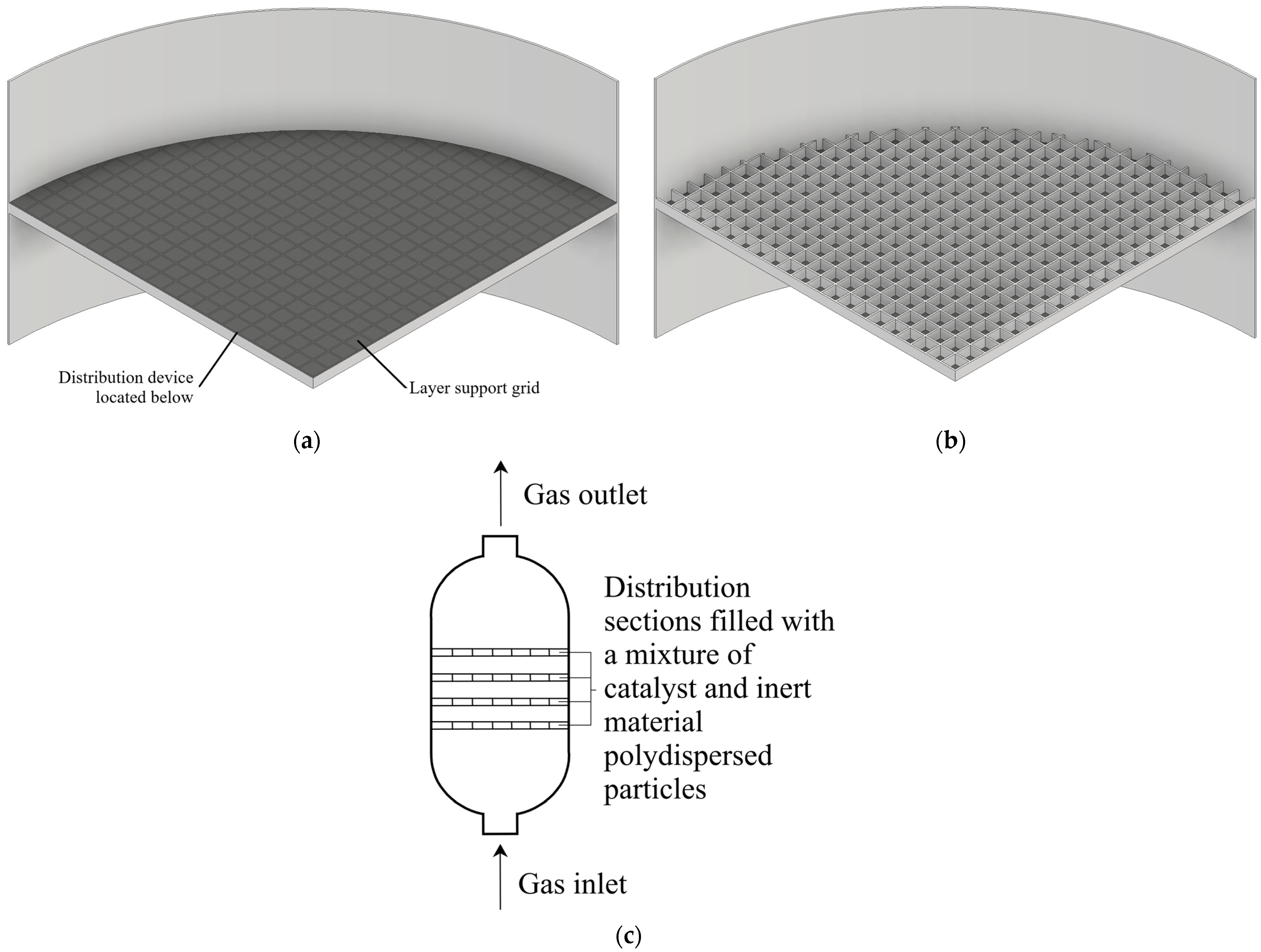
2.1. Object of Study

The object of the study is a reactor with a fluidized bed of catalyst particles and inert particles (those particles and the other ones, as well as the mixture thereof, hereinafter referred to as particles) which are located on distribution grids. Figure 2b,c show a schematic representation of the distribution device proposed in this work.

The diameter of the zone where the particles are located is 3 m. The grid is made of vertically arranged plates 60 mm high and 10 mm thick, and the distance between the plates is 90 mm. The parameters of catalyst and inert material hypothetical particles presented in

Table 2. Parameters of catalyst and inert material particles.

Name of the Parameter	Parameter Value
Catalyst particle size, mm	1.5–3.0 *
Apparent density of catalyst particles, kg/m3	2500
Heat capacity of catalyst particles, J/(kg∙K)	962.6
Volume fraction of catalyst in the catalyst–inert material mixture, %	20
Particle size of inert material, mm	2–4 *
Apparent density of inert material particle, kg/m3	2200
Heat capacity of particles of inert material, J/(kg∙K)	879.7

* the particle size distribution was determined by the Rosin–Rammler powder law [61].

are the average values of the parameters of the particles presented in the patent [62]. The liquefying medium is gas (air).

2.2. Research Methods

All the results presented in this work were obtained using the ANSYS Fluent 2021R1 CFD package. This software package has a wide set of models that allows one to fully solve the tasks.

Since the entire particle bed is located in the cells of the distribution device, presumably “free” fluidization will be observed “locally” in each cell formed by the distribution grid (Figure 2b, Figure 3 and Figure 4) individually and not throughout the entire section of the reactor. For this reason, it was decided to simulate only one cell, and not the entire section of the apparatus.

Simulating a single cell rather than an entire layer allows the researchers to achieve the following:

• to conduct three-dimensional simulation, since the reduced scale frees up a significant amount of computing power;
• to use more precise models, such as the Unresolved Discrete Particle Model (UDPM), and Resolved Discrete Particle Model (RDPM), which are not capable of simulating objects larger than the laboratory size. In this work, preference was given to UDPM, since, according to the assumptions obtained, the interaction of particles between themselves and the walls, and not between gas and particles, plays a decisive role in the behavior of the particle bed;
• to reduce the total time of each calculation, which allows one to make more calculations to collect more detailed information about the system.

The following models were chosen to solve all the problems:

• a multiphase model: DPM [49]; the gas-particle drag law of Wen and Yu [49];
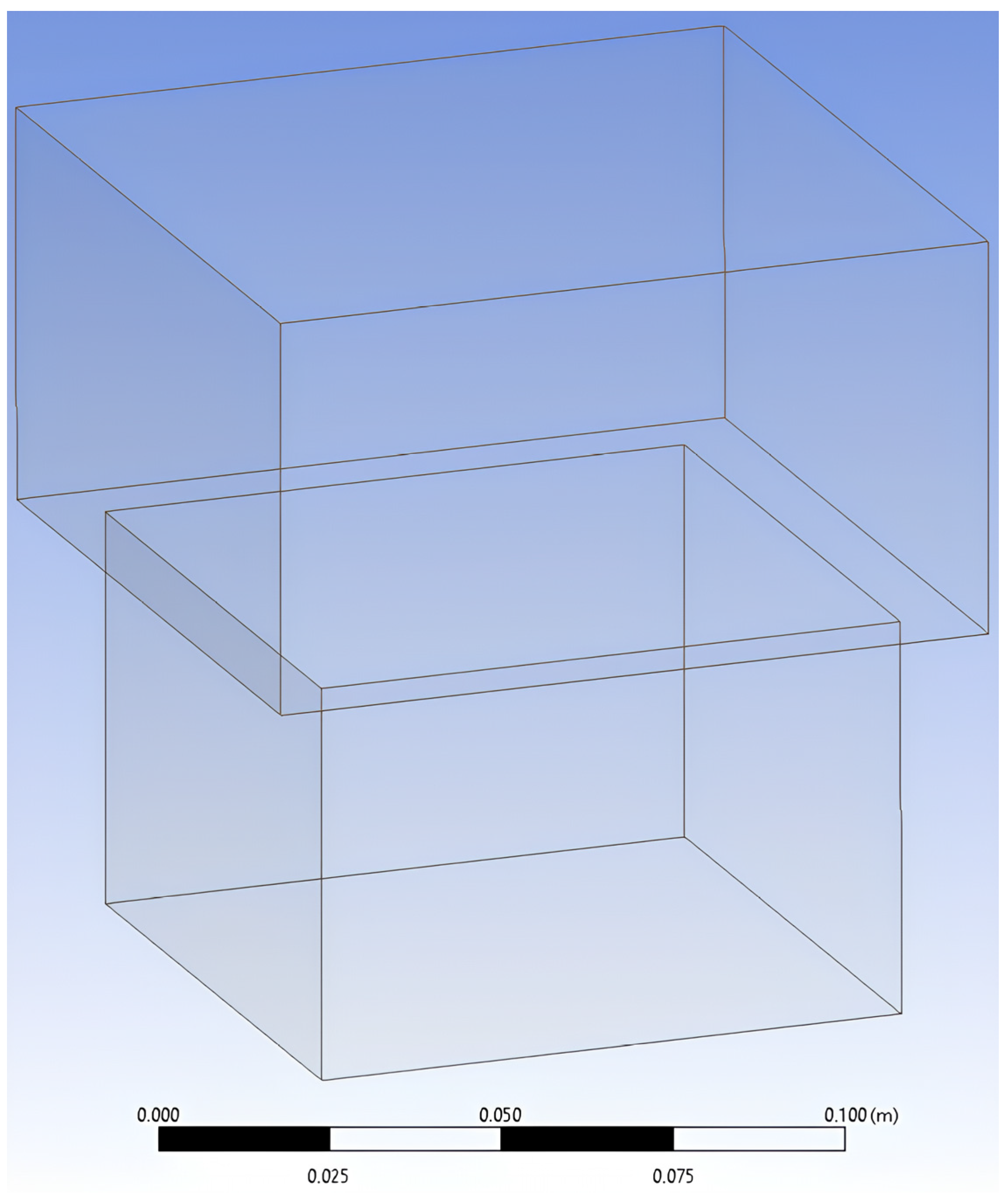
• for DPM: the rheological “spring-damper” scheme determines the nature of collisions of the particles with objects. In this case it implies an inelastic collision; for the particle–plane symmetry pair, an ideally elastic collision was chosen. The lateral faces of the upper part of the simulated cell (Figure 4) were set as planes of symmetry, since they represent the gas–gas interface planes, i.e., there is a gas phase in front of and behind the plane;
• a turbulence model: the realizable k-ε model with restriction of the turbulence kinetic energy generation term and viscous heating to make calculations taking heating into account [49].

Since ANSYS Fluent uses the finite volume method, i.e., the entire volume of the modeled object is divided into many elements of various shapes (tetrahedron, hexahedron, polyhedron, etc.), it is necessary to determine the minimum size of the element of the final mesh, which is also called the Euler mesh. For UDPM, it is necessary for the minimum size of the Euler mesh to exceed the size of the largest particle; in our case, these inert material particles are 4 mm in diameter. However, the considered problem also includes particles that have a smaller size, but an excessively large mesh will lead to a larger number of particles happening to be in one ensemble, so simulation of their movement would be incorrect. Therefore, the minimum size of 6 mm of the mesh elements for the tetrahedral shape of the elements was chosen. The view of the obtained mesh is shown in Figure 3; it has a minimum orthogonality of 0.353 (the minimum value of the cosine of the angle between the normal to the cell face and the line connecting the centers of neighboring cells), the maximum aspect ratio is 8.56, and the minimum asymmetry is 0.43. Figure 4 shows the created research area (cells of the reactor distribution grid): the dimensions of the lower part are 90 × 90 × 60 mm (axes dimensions, see Figure 3); and the dimensions of the upper part are 110 × 110 × 80 mm. In the proposed design of the reaction zone, the lower part is limited by vertical baffles, and the upper part with “expansion” has no physical boundaries. Therefore, the side faces of the model in this area were set as symmetry. The absence of solid baffles allows the gas flow in this area to be redistributed which leads to the destruction of bubbles and mixing of catalyst particles. This avoids the slugging regime while preserving the advantages of the arranged fluidized bed.

Further, a study was carried out on the grid independence to confirm that the size of the finite elements of the grid is small enough. Two more models with a larger and smaller minimum mesh size were made. All three models were named according to the number of elements in the mesh. Since the value chosen is only the lower limit and the elements may have a larger size, albeit not much larger than the specified threshold, this will lead to a disproportionate change in the element number when the limit value changes. The first mesh has ~5500 cells with a minimum mesh element size of 9 mm.; the second mesh has ~18,000 cells with a minimum mesh element size of 6 mm; and the third mesh has ~34,000 cells with a minimum mesh element size of 4.5 mm. To compare the calculation results, the value of the area-weighted average pressure at the inlet of the cell (inlet from below) was used for one second of simulation. The simulation time, as well as the gas velocity of 1.5 m/s, were randomly chosen. The results are shown in Figure 5.

Based on the results of comparing the area-weighted average pressure at the inlet of the distribution device cell, the mesh of 18,000 cells was selected for further calculations. It can be seen from Figure 5 that with an almost two-fold increase in the number of mesh cells as compared to the mesh we selected, the pressure pulsations have practically not changed in magnitude, but there is a shift of phase fluctuations, which is explained by a more accurate calculation of gas flows between particles due to a smaller mesh. However, such an increase in the number of elements has not led to a significant improvement in the results, and the calculation time has increased by several times. The reverse is the case for the model with the 5500 cell: a small number of cells have increased the calculation speed, but excessively large elements do not allow sufficient calculation of interparticle gas flows with significantly higher velocity than that at the inlet, and as a result, the layer remained fixed.

2.2.1. Gas and Particle Motion Models

As noted in the introduction, in the CFD-DEM model, gas is modeled using the Euler approach, and particles are modeled using the Lagrange approach. The gas flow is described by two basic equations: the law of conservation of mass (or the continuity Equation (2)) and the law of conservation of momentum (or the Navier–Stokes Equation (3)) [63,64,65]:

$$\frac{\mathsf{\partial }\rho }{\mathsf{\partial }t}+\nabla \cdot \left(\rho \overrightarrow{u}\right)=S_m,$$

(2)

where $\rho$ is the gas density; $\overrightarrow{u}$ is the gas velocity; S_m is the source term that determines the mass added from the dispersed second phase or another source (for instance, evaporation of liquid droplets); and t is the time;

$$\frac{\mathsf{\partial }}{\mathsf{\partial }t}\left(\rho \overrightarrow{u}\right)+\nabla \cdot \left(\rho \overrightarrow{u}\overrightarrow{u}\right)=-\nabla p+\nabla \cdot \left(\overline{\overline{\tau }}\right)+\rho \overrightarrow{g}+\overrightarrow{F},$$

(3)

where p is the static pressure; $\overline{\overline{\tau }}$ is the stress tensor; $\overrightarrow{g}$ is acceleration of gravity; and $\rho \overrightarrow{g}$ and $\overrightarrow{F}$ are the gravitational and external volumetric forces.

The equation of the stress tensor has the following form:

$$\overline{\overline{\tau }}=\mu \left[\left(\nabla \overrightarrow{u}+\nabla {\overrightarrow{u}}^T\right)-\frac{2}{3}\nabla \cdot \overrightarrow{u}I\right],$$

(4)

where μ is the molecular viscosity; T is the transposition of the vector; I is the unit tensor; and the second term of the right side of the equation is responsible for the effect of volume dilation.

However, DEM can be divided into resolved (RDPM) and unresolved (UDPM). For RDPM, the gas flow is calculated on a computational mesh around particle boundaries which become solid boundaries. This approach is very detailed, which requires significant computing power for simulating systems of practical scale [66]. For the possibility of simulating larger systems, UDPM is used [67]. This model calculates the average volume values of the velocity and density of the gas, while the volume of the mesh element should exceed the particle size by several times. Equations (2) and (3) averaged by volume have the following form [68]:

$$\frac{\mathsf{\partial }\left(\rho {\epsilon }_p\right)}{\mathsf{\partial }t}+\nabla \cdot \left(\rho {\epsilon }_p\overrightarrow{u}\right)=S_m,$$

(5)

$$\frac{\mathsf{\partial }}{\mathsf{\partial }t}\left(\rho {\epsilon }_p\overrightarrow{u}\right)+\nabla \cdot \left(\rho {\epsilon }_p\overrightarrow{u}\overrightarrow{u}\right)=-{\epsilon }_p\nabla p+\nabla \cdot \left(\overline{\overline{\tau }}\right)\cdot \epsilon +\rho {\epsilon }_p\overrightarrow{g}+\overrightarrow{F}+{\overrightarrow{F}}_{drag},$$

(6)

where ${\epsilon }_p$ is the porosity of the particle bed and ${\overrightarrow{F}}_{drag}$ are the drag forces. It should be noted that to calculate the drag forces, closing expressions are required; the type depends on the chosen DEM approach: soft or hard spheres [68].

The porosity of the particle bed is determined by the Particle Centroid Method (PCM). The particle affects the porosity value of the particle bed only of that cell of the computational mesh where its center is located:

$${\epsilon }_p=1-\frac{{\displaystyle \sum n_{p,i}}\cdot V_{p,i}}{V_{\mathsf{\Omega }}},$$

(7)

where $n_{p,i}$ is the volume fraction of the i-th particle of the cell; $V_{p,i}$ is the volume of the i-th particle; and $V_{\mathsf{\Omega }}$ is the volume of the cell for which the porosity value of the particle bed ${\epsilon }_p$ is calculated.

In turn, the particles are described by the equations of force balance (8) and momentum balance (11) [49]:

$$m_p\frac{d{\overrightarrow{u}}_p}{dt}=m_p\frac{\overrightarrow{u}-{\overrightarrow{u}}_p}{{\tau }_r}+m_p\frac{\overrightarrow{g}\left({\rho }_p-\rho \right)}{{\rho }_p}+\overrightarrow{F},$$

(8)

where m_p is the mass of particles; ${\overrightarrow{u}}_p$ is the velocity of particles; ${\rho }_p$ is the density of particles; the first term of the right side of the equation is the drag force; and ${\tau }_r$ is the relaxation time of particles. ${\tau }_r$ is calculated by the following formula [69]:

$${\tau }_r=\frac{{\rho }_p{d}_p^2}{18\mu }\cdot \left(\frac{24}{C_d\mathrm{Re}}\right),$$

(9)

where d_p is the diameter of the particles; and Re is the relative Reynolds number. It is determined by the following formula [49]:

$$\mathrm{Re}\equiv \frac{\rho d_p\left|{\overrightarrow{u}}_p-\overrightarrow{u}\right|}{\mu }.$$

(10)

To consider the rotation of the particle, an additional ordinary differential equation of the angular momentum of the particle was solved [49]:

$$I_p\frac{d{\overrightarrow{\omega }}_p}{dt}=\frac{\rho }{2}{\left(\frac{d_p}{2}\right)}^5{C}_{\omega }\left|\overrightarrow{\mathsf{\Omega }}\right|\overrightarrow{\mathsf{\Omega }}=\overrightarrow{T},$$

(11)

where $I_p$ is the moment of inertia; ${\overrightarrow{\omega }}_p$ is the particle angular velocity; $C_{\omega }$ is the rotation drag coefficient; $\overrightarrow{T}$ is the torque applied to the particle; and $\overrightarrow{\mathsf{\Omega }}$ is the angular velocity of the particle relative to the gas. $\overrightarrow{\mathsf{\Omega }}$ is determined by the following formula:

$$\overrightarrow{\mathsf{\Omega }}=\frac{1}{2}\nabla \times \overrightarrow{u}-{\overrightarrow{\omega }}_p.$$

(12)

2.2.2. Turbulence Model

In this work, a realizable k-ε turbulence model was applied, since it suits a number of mathematical restrictions imposed on Reynolds stresses. These restrictions are consistent with the physics of real turbulent flows. Neither the standard nor the RNG (Re-Normalization Group) model are “realizable”, i.e., the denominator of one of the terms can turn to zero in the equation of kinetic energy dissipation of turbulence [49].

The realizable k-ε turbulence model is based on the standard k-ε model, which is semi-empirical [61]. The standard k-ε model includes two separate equations for the transfer of the kinetic energy of turbulence k and its dissipation rate ε. Since the transport equation for ε is obtained empirically, it bears little resemblance to an exact mathematical counterpart, compared with the equation for k [49]:

$$\frac{\mathsf{\partial }}{\mathsf{\partial }t}\left(\rho k\right)+\nabla \cdot \left(\rho k\overrightarrow{u}\right)=\nabla \cdot \left[\left(\mu +\frac{{\mu }_t}{{\sigma }_k}\right)\nabla k\right]+G_k+G_b-\rho \epsilon +Y_M+S_k,$$

(13)

$$\frac{\mathsf{\partial }}{\mathsf{\partial }t}\left(\rho \epsilon \right)+\nabla \cdot \left(\rho \epsilon \overrightarrow{u}\right)=\nabla \cdot \left[\left(\mu +\frac{{\mu }_t}{{\sigma }_{\epsilon }}\right)\nabla \epsilon \right]+C_{1\epsilon }\frac{\epsilon }{k}\left(G_k+C_{3\epsilon }{G}_b\right)-C_{2\epsilon }\rho \frac{{\epsilon }^2}{k}+S_{\epsilon },$$

(14)

where ${\mu }_t$ is the turbulent viscosity; ${\sigma }_k, {\sigma }_{\epsilon }$ are the turbulent Prandtl numbers for k and ε, respectively; $G_k$ is the generation of the kinetic energy of turbulence caused by the velocity gradient; $G_b$ is the generation of the kinetic energy of turbulence caused by buoyancy; $Y_M$ is the contribution of dilatational dissipation to the total rate of dissipation of turbulence kinetic energy for compressible flows; $C_{1\epsilon }, C_{2\epsilon }, C_{3\epsilon }$ are constants; and $S_k, S_{\epsilon }$ are user-defined source terms.

The turbulent viscosity in the realizable k-ε turbulence model is calculated based on the values of k and ε [49]:

$${\mu }_t=\rho C_{\mu }\frac{k^2}{\epsilon },$$

(15)

where $C_{\mu }$ is the constant.

To prevent the denominator of one of the terms from tending to zero in the dissipation equation for turbulence kinetic energy, two changes were introduced in the realizable k-ε turbulence model compared to the standard k-ε model [49]:

• the turbulent viscosity formula now includes the variable originally proposed by Reynolds;
• the dissipation equation has been changed, based on the dynamic equation of the mean-square vorticity fluctuation.

The transport equation for k in the realizable k-ε turbulence model is identical to the transport equation for k in the standard k-ε turbulence model. The transport equation for ε has the following form [66]:

$$\frac{\mathsf{\partial }}{\mathsf{\partial }t}\left(\rho \epsilon \right)+\nabla \cdot \left(\rho \epsilon \overrightarrow{u}\right)=\nabla \cdot \left[\left(\mu +\frac{{\mu }_t}{{\sigma }_{\epsilon }}\right)\nabla \epsilon \right]+\rho C_1{S}_{\epsilon }-\rho C_2\frac{{\epsilon }^2}{k+\sqrt{v\epsilon }}+C_1\frac{\epsilon }{k}{C}_3{G}_b+S_k,$$

(16)

where

$$C_1=\max \left[0.43; \frac{n}{n+5}\right],$$

(17)

$$n=S\frac{k}{\epsilon }; S=\sqrt{2S_{ij}{S}_{ij}},$$

(18)

where $S_{ij}$ is the mean strain rate tensor; and S is a scalar invariant of the strain rate tensor.

It should be noted that the second term on the right side of Equation (16), despite other turbulence models, does not generate turbulence kinetic energy.

The equation for calculating turbulent viscosity does not differ from the similar equation for the standard k-ε model, except for $C_{\mu }$ being no longer the constant, and it is calculated by the formula [49,53]:

$$C_{\mu }=\frac{1}{A_0+A_s\frac{k{U}^{*}}{\epsilon }},$$

(19)

where

$$U^{*}=\sqrt{S_{ij}{S}_{ij}+{\tilde{\mathsf{\Omega }}}_{ij}{\tilde{\mathsf{\Omega }}}_{ij}},$$

(20)

where ${\tilde{\mathsf{\Omega }}}_{ij}$ is the mean rate-of-rotation tensor viewed in a moving reference frame with the angular velocity ${\omega }_k$; j and k are item numbers of the basis coordinate vectors; and ${\epsilon }_{ijk}$ is the Levi-Civita symbol. The constants of the model $A_0, A_s$ are given by the formulas:

$$A_0=4.04; A_s=\sqrt{6}\cos \left(\phi \right),$$

(21)

where

$$\phi =\frac{1}{3}{\cos }^{-1}\left(\sqrt{6}W\right),$$

(22)

$$W=\frac{S_{ij}{S}_{jk}{S}_{ki}}{{\tilde{S}}^3},$$

(23)

$$\tilde{S}=\sqrt{S_{ij}{S}_{ij}},$$

(24)

$$S_{ij}=\frac{1}{2}\left(\frac{\mathsf{\partial }{u}_j}{\mathsf{\partial }{x}_i}+\frac{\mathsf{\partial }{u}_i}{\mathsf{\partial }{x}_j}\right),$$

(25)

where $\tilde{S}$ is the modulus of the mean strain rate tensor.

2.2.3. Heat Transfer

ANSYS Fluent solves the following energy equation [49]:

$$\frac{\mathsf{\partial }}{\mathsf{\partial }t}\left(\rho \left(e+\frac{v^2}{2}\right)\right)+\nabla \cdot \left(\rho v\left(h+\frac{v^2}{2}\right)\right)=\nabla \cdot \left(k_{eff}\nabla T-{\displaystyle \sum _j{h}_j\overrightarrow{J_j}+{\overline{\overline{\tau }}}_{eff}\cdot \overrightarrow{v}}\right)+S_h,$$

(26)

where $\overrightarrow{J_j}$ is the diffusion flux of species j; and h is enthalpy. $k_{eff}$ is determined by the following formula:

$$k_{eff}=k+k_t,$$

(27)

where $k_t$ is the turbulent thermal conductivity, determined depending on the selected turbulence model. The first term of Equation (26) represents energy transfer due to thermal conductivity, the second term due to the diffusion of molecules, and the third term due to viscous energy dissipation. The source term $S_h$ is responsible for user-defined volumetric heat sources or for the thermal effects of ongoing reactions. It also involves the exchange of energy between the discrete and continuous phases. h in Equation (26) is determined by the following formula:

$$h={\displaystyle \sum _j{Y}_j{h}_j},$$

(28)

where $Y_j$ is the mass fraction of species j and the sensible heat of species $h_j$ is the part of enthalpy that includes only changes in the enthalpy due to specific heat:

$$h_j={\displaystyle {\int }_{T_{ref}}^T{c}_{p,j}dT},$$

(29)

where $c_{p,j}$ is the heat capacity of species j; and the reference temperature value $T_{ref}$ depends on the chosen solver and model in use for the pressure-based solver; the value is 298.15 K.

The calculation of energy transfer between the discrete and continuous phases is carried out locally for each cell of the computational mesh. The equation of transferred energy without taking into account chemical reactions has the following form [49]:

$$Q=\frac{{\dot{m}}_{p,0}}{m_{p,0}}\left[\left(m_{p_{in}}-m_{p_{out}}\right)\left[-H_{la{t}_{ref}}+H_{pyrol}\right]-m_{p_{out}}{\displaystyle {\int }_{T_{ref}}^{T_{p_{out}}}{c}_{p_p}dT+m_{p_{in}}{\displaystyle {\int }_{T_{ref}}^{T_{p_{in}}}{c}_{p_p}dT}}\right],$$

(30)

where the indices in and out denote the parameters on cell entry and cell exit; ${\dot{m}}_{p,0}$ is the initial mass flow rate of the particle injection; $m_{p,0}$ is the initial mass of the particle; $m_p$ is the mass of the particle; $c_{p_p}$ is the heat capacity of the particle; $H_{pyrol}$ is the heat of pyrolysis as volatiles are evolved; $T_p$ is the temperature of the particle; and $H_{la{t}_{ref}}$ is the latent heat at reference conditions.

The Nusselt number in the case of granular flows is determined by the following equation:

$$Nu=\left(7-20{\alpha }_f+5{\alpha }_f^2\right)\left(1+0.7{\mathrm{Re}}^{0.2}{\mathrm{Pr}}^{1/3}\right)+\left(1.33-2.4{\alpha }_f+1.2{\alpha }_f^2\right){\mathrm{Re}}^{0.7}{\mathrm{Pr}}^{1/3},$$

(31)

where ${\alpha }_f$ is the thermal conductivity in the liquid phase and Pr is the Prandtl number.

3. Results

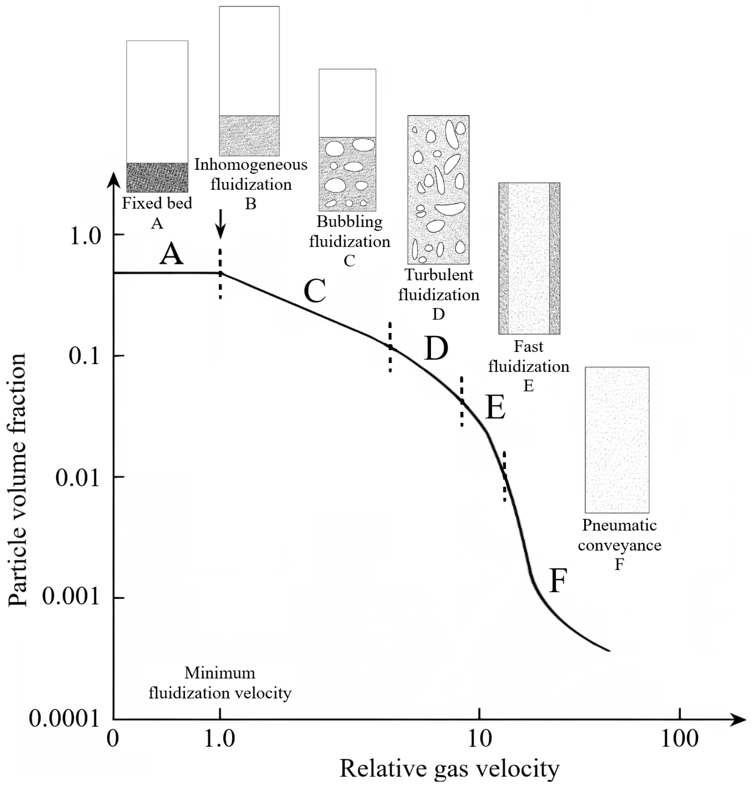
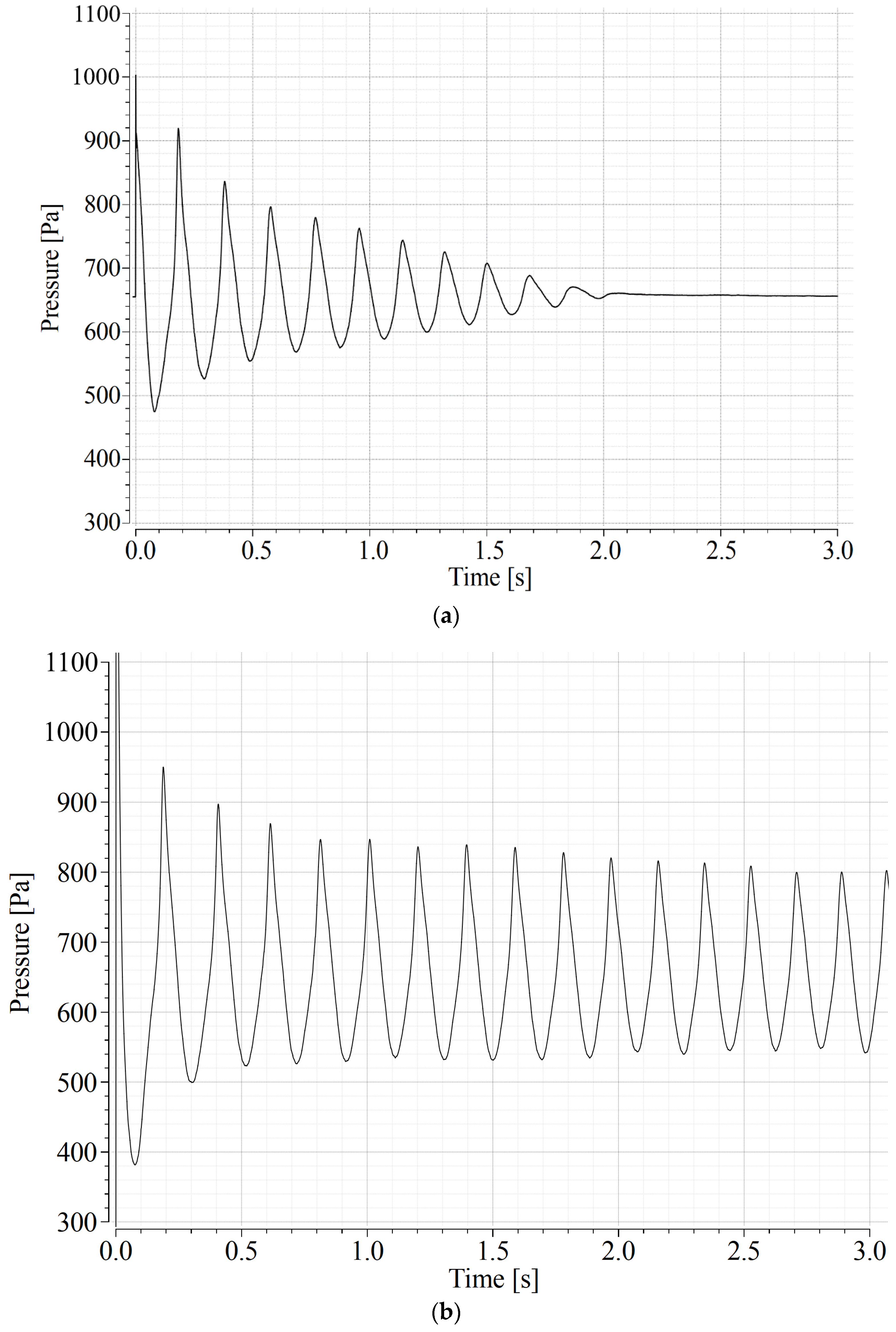
3.1. Determination of the Minimum Fluidization Velocity

The first step of the study was to determine the minimum fluidization velocity. The behavior of the particle layer was modeled under the following conditions. There were ~25,000 particles in the distribution device cell, the initial gas velocity was 0 m/s, and the gas velocity at the inlet of the distribution device cell gradually increased according to the law a·t (where t is the time from the initial state of the system, s; and a is the acceleration, 0.4 m/s²). As a result of the simulation, the hydraulic resistance of the particle layer was determined.

Figure 6 shows the moment when the pressure under the particle layer ceases to change with time, which shows that the minimum fluidization velocity has been reached. The gas velocity, when it was achieved, has become ~1 m/s. A further increase in the gas velocity leads to an increase in the height of the particle layer.

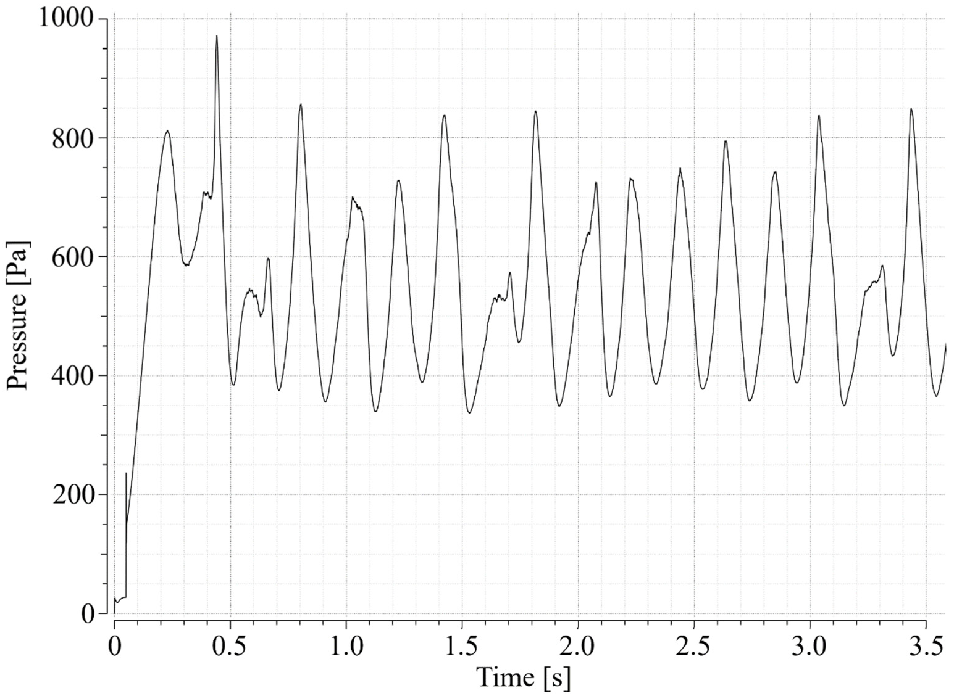
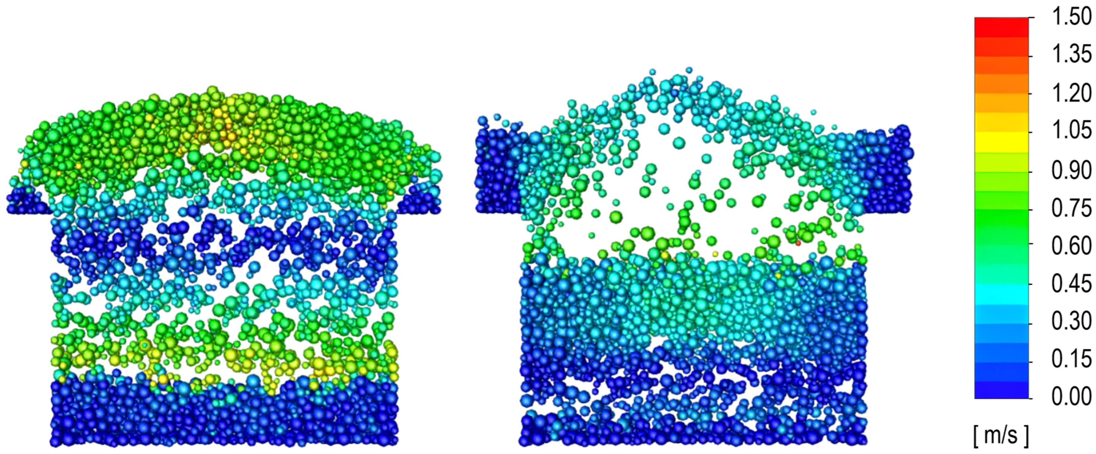
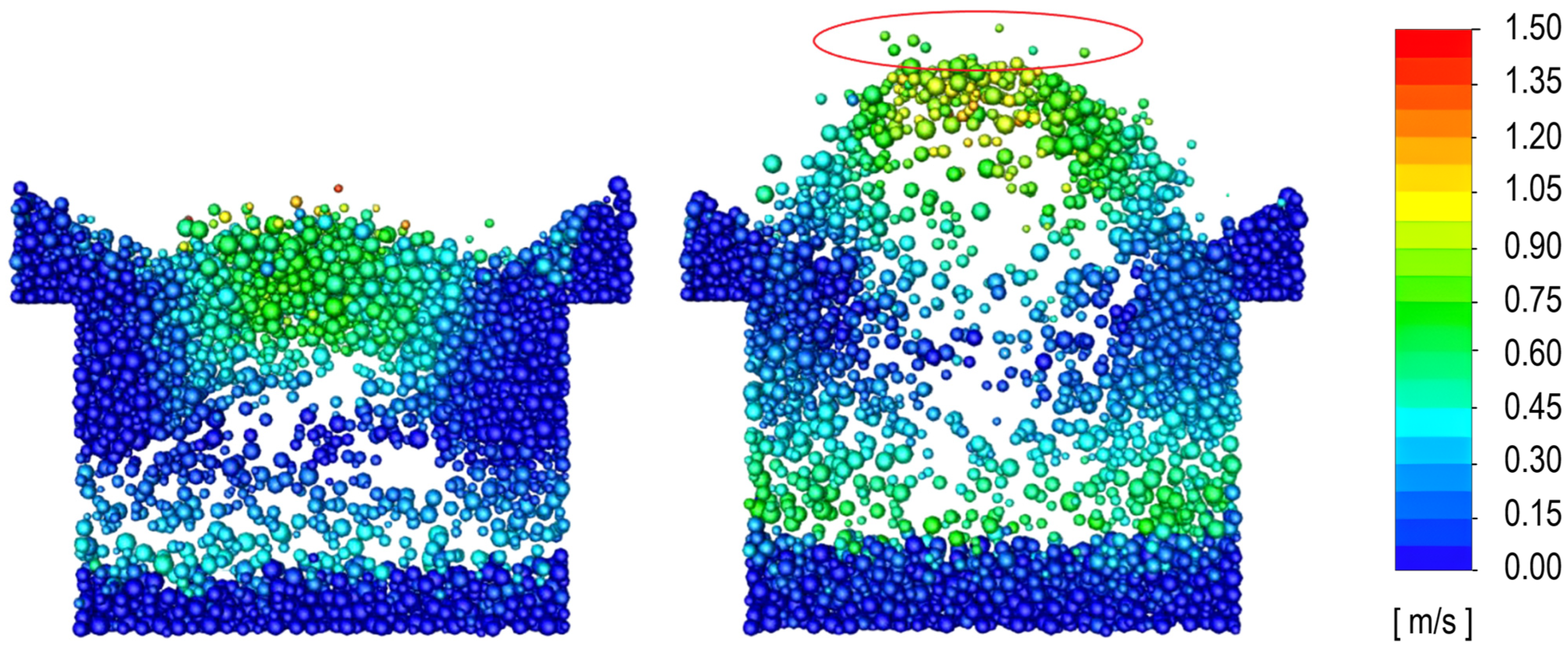
3.2. Determination of the Minimum Velocity of Bubbling Regime

Further, a series of calculations was carried out to determine the minimum gas velocity at which the regime becomes bubbling. These calculations are necessary because the grid forms relatively narrow channels, and the layer may tend to be in the slugging regime at velocities slightly higher than the minimum required fluidization velocity. It was determined that when the gas velocity reaches 1.4 m/s and higher, then the periodic undamped pressure fluctuations are observed (Figure 7b).

According to the visualization of the solution presented in Figure 8, it can be seen that the formed gas bubbles occupy the entire cross-section of the simulated cell, i.e., the fluidized bed with slugging fluidization is observed. This is due to the narrow space (in our case, the narrowness of the distribution grid cells) and the relatively large particle size (see Section 1). That is, macrostructures, such as gas bubbles, occupy the entire horizontal cross-section of the distribution device cell. Such a regime has a negative effect on the processes in the bed, since it excludes the mixing of particles, and, at the same time, it has significant uniformity (strictly periodic pressure fluctuation). To switch over from this fluidization to a bubbling or turbulent regime, it is necessary to increase the gas velocity.

However, the simulation was carried out only for one cell of one particle layer, and the loss of gas velocity due to hydraulic resistance should be taken into account in order to ensure the bubbling of the upper layers of particles. To do this, it is necessary to increase the gas velocity at the inlet up to such values that the velocity would be greater than 1.4 m/s at the inlet of the last layer of particles. It was found that when passing through the particle layer, the gas velocity drops by ~17%, from 1.4 m/s to 1.1–1.2 m/s, as shown in Figure 9.

However, it should be noted that with a significant increase in gas velocity at the inlet to the first layer, the particles will be carried away and they will beat against the support grid of the second layer, which can cause their destruction or rapid erosion. This is a restriction of the number of granular material layers. Based on the simulation results shown further in Figure 10, Figure 11, Figure 12 and Figure 13, it is noticeable that some particles are close to hitting at the support grid of the next layer. The upper group of seven particles in Figure 13 (highlighted in red) at t = 0.57 s is located at a distance of under 1.5 cm from the support grid. Hence, an increase in gas velocity above 3 m/s is impractical. Since it is necessary to ensure the bubbling regime of the upper particle layers, taking into account the layer hydraulic resistance losses, therefore, the optimal number of layers equal to four was adopted.

Having assumed that the gas will lose ~17% of the velocity in each layer of particles, 3 m/s was chosen as the optimal value. The simulation results obtained, namely inlet pressure and visualization of particle positions and velocities, are shown in Figure 10, Figure 11, Figure 12 and Figure 13 at 0, 0.15, 0.39, 0.45, 0.54, and 0.57 s, respectively. The time intervals are a random choice. From the data presented, it can be seen that an increase in gas velocity by more than two times significantly affected both the fluidization regime and its uniformity (pressure fluctuations became chaotic, Figure 10). The regime approached the turbulent fluidization; however, as the gas velocity decreased due to the hydraulic resistance of the layers, the fluidization uniformity increased.

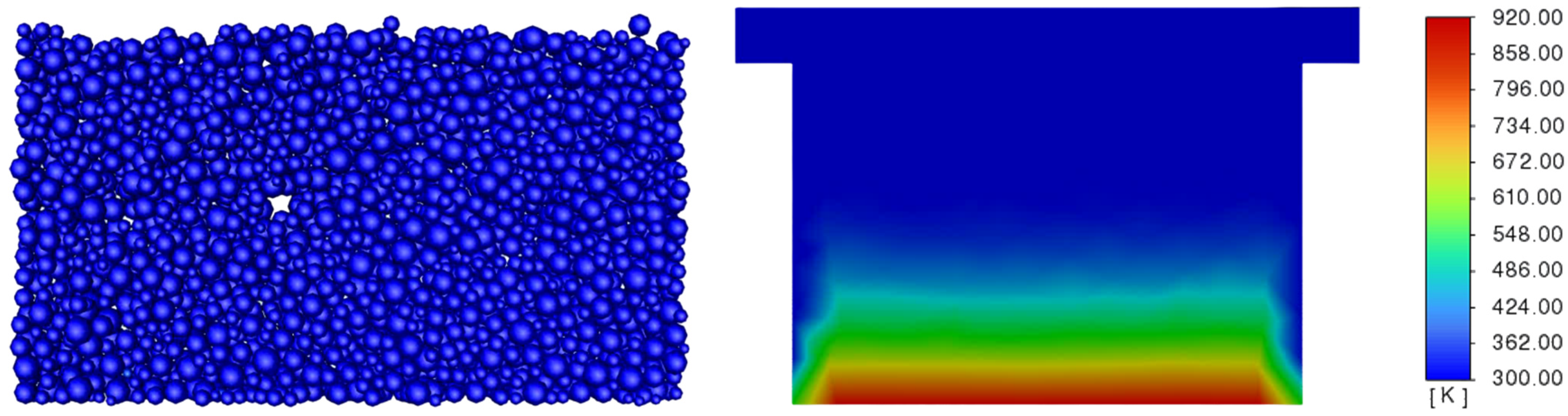
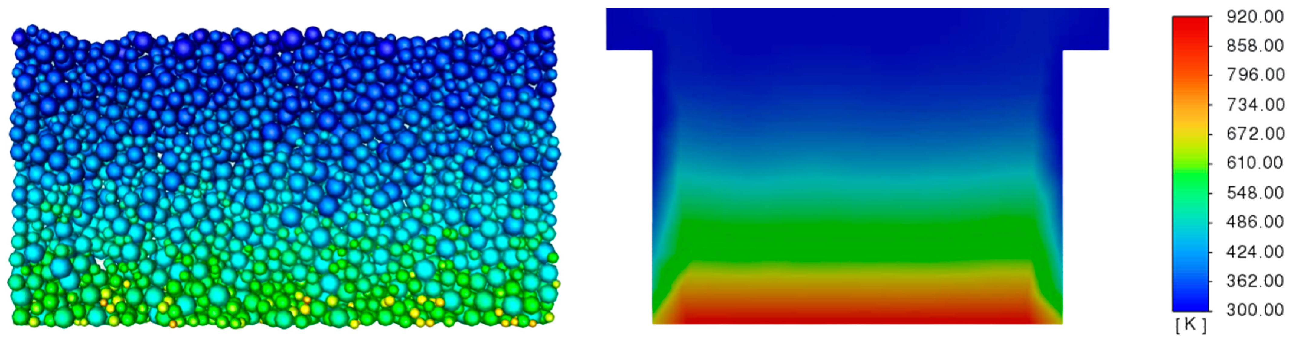
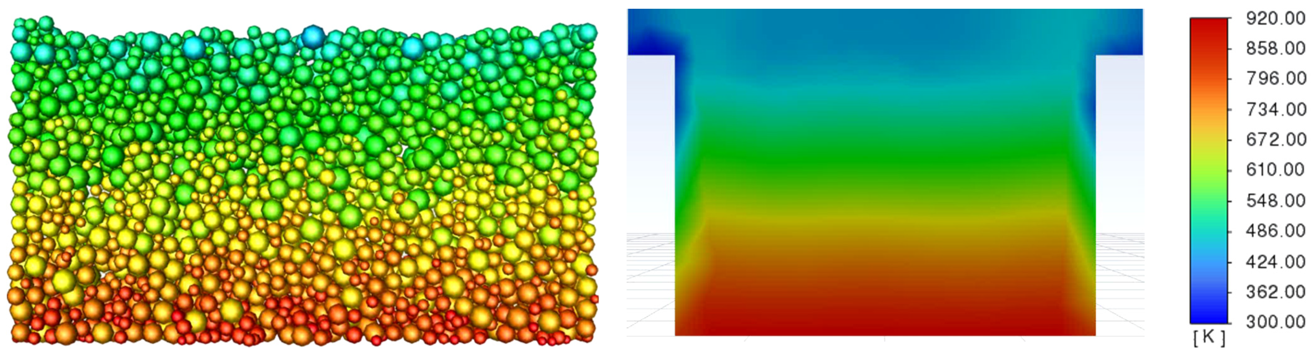
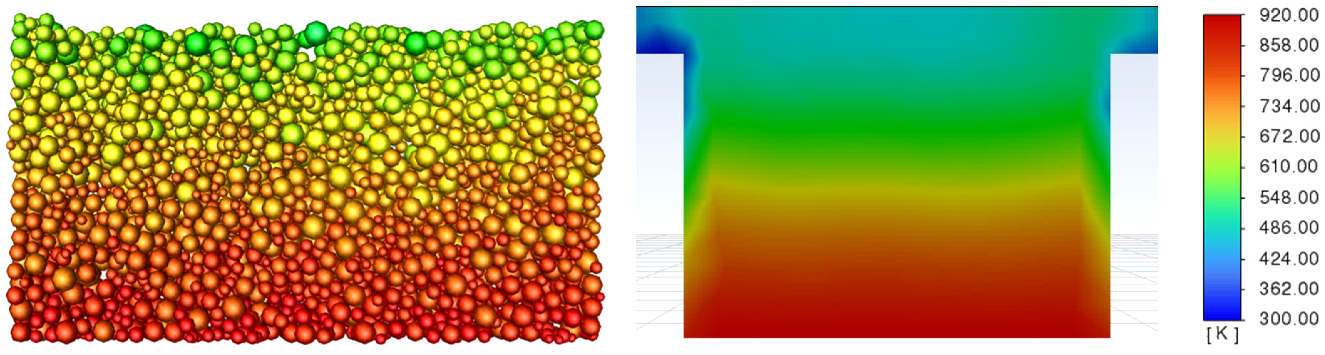
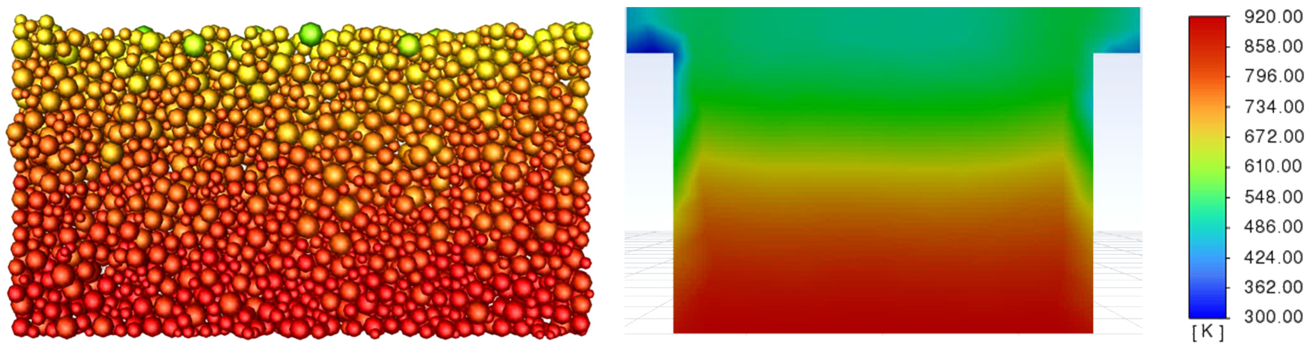
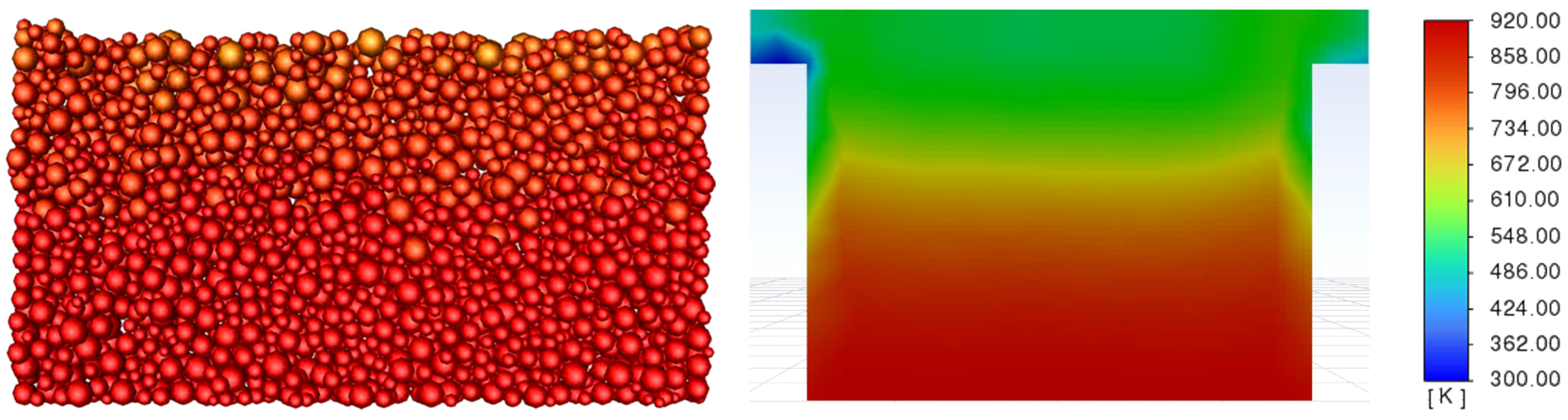
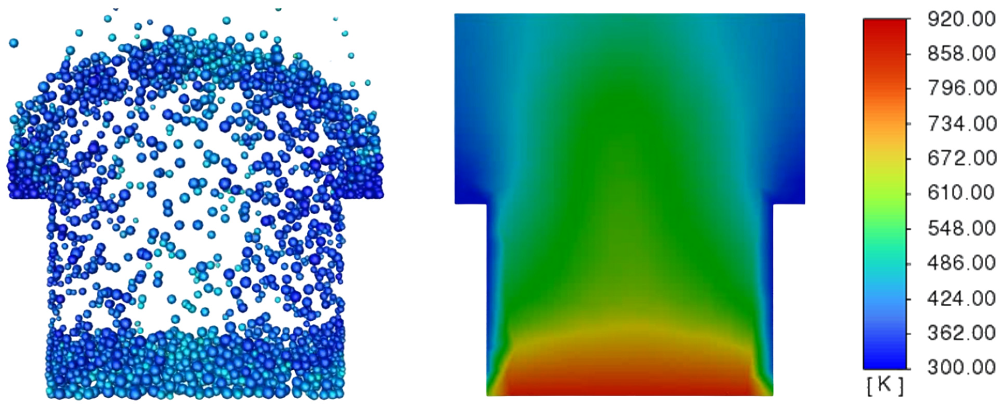
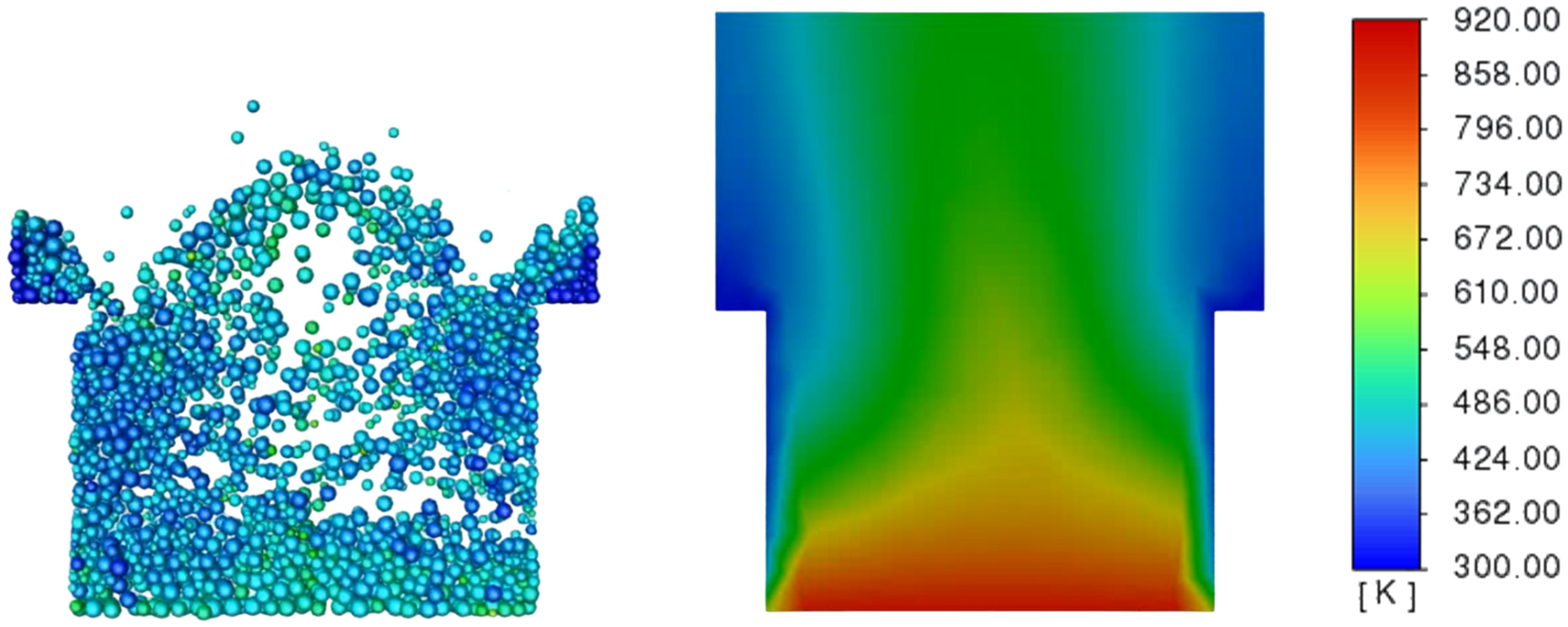
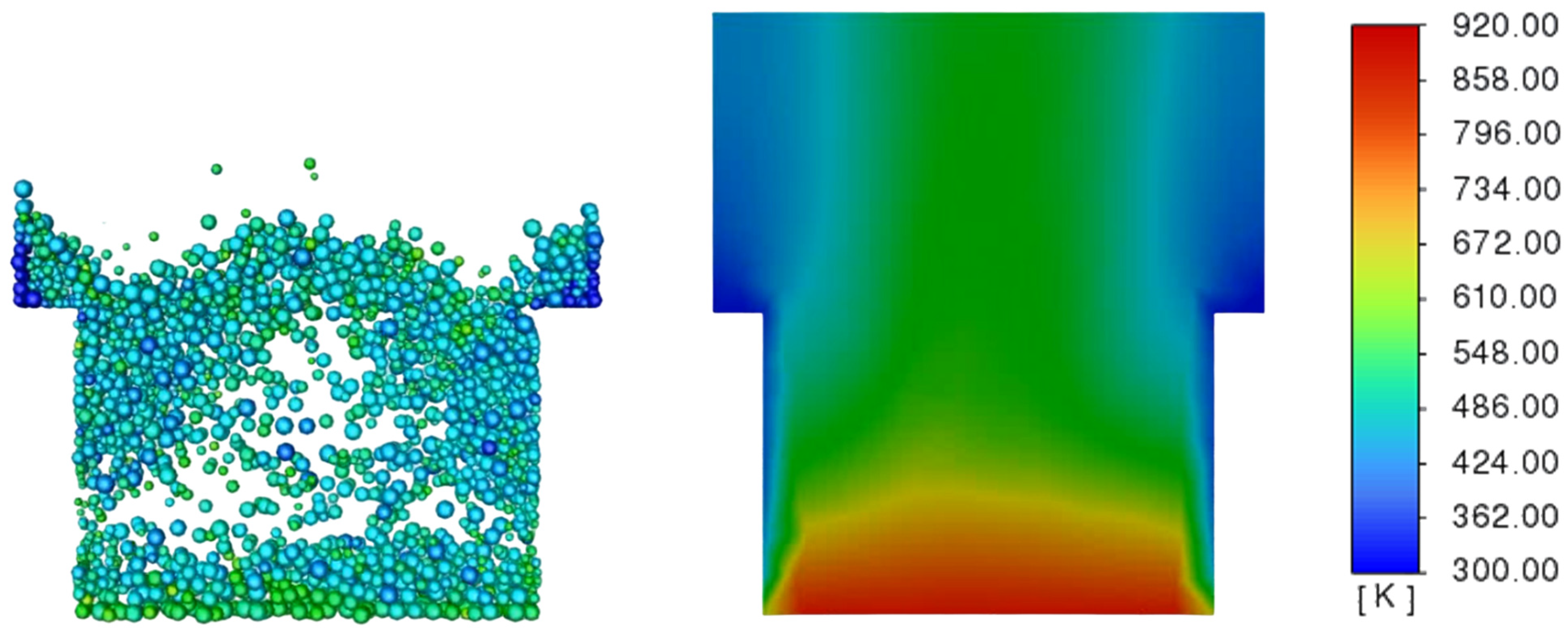
3.3. Determination of the Effect of the Fluidization Regime on Particle Heating and the Effect of High Gas Temperature on the Fluidization Regime Itself

Further, simulation of particle heating at a temperature of 923 K, which is the average value of the temperature range of the high-temperature catalytic combustion of exhaust gases, was carried out [68]. The gas velocity was assumed to be equal to the minimum fluidization velocity (1 m/s), which would allow for a visual comparison of heating of the stationary and bubbling layer. The approximate heating time of the entire particle layer was about 72 s. Figure 14, Figure 15, Figure 16, Figure 17, Figure 18 and Figure 19 shows the results of simulating the process at certain times from the beginning of the simulation, namely 0, 5.85, 24, 36, 48, and 72 s respectively.

According to Figure 14, Figure 15, Figure 16, Figure 17, Figure 18 and Figure 19, it can be seen that at the middle of the process, almost half of the solid phase has been heated up to the required temperature. As the particles heat up, the temperature difference between them and the gas decreases, and at the same time the driving force of the heat transfer decreases, which leads to a significant increase in the heating process time for this layer.

From about 24 s of the process, the gas flow would not transfer all its heat to the particles (i.e., at the outlet of the particle layer, the gas had a higher temperature than the particles in the upper part of the layer, which is noticeable on the gas temperature contour starting from Figure 15). This heat rises with the flow to the next layer of particles and is spent on heating the layer. Thus, if 72 s are spent on heating the first layer of particles from the beginning of the process, then it requires less than 144 s to heat the two layers of particles (two times 72 s). Based on this, we believe that the heating time of all particle layers under current conditions will be less than 288 s (four times 72 s).

The process can be accelerated by carrying it out in a bubbling regime. The greater gas consumption, its active mixing with particles, and their uniform heating will ensure a higher temperature difference between the gas and the particles (i.e., the driving force of the heat transfer process increases), despite the reduced contact time caused by the increased gas velocity.

Further simulation was carried out under the same conditions as the previous one, except for the gas velocity, which was increased to 3 m/s. The results obtained are shown in Figure 20, Figure 21, Figure 22 and Figure 23.

According to Figure 20, Figure 21, Figure 22 and Figure 23, it can be seen that a three-fold increase in the gas velocity has not led to a proportional increase in the particle heating rate. This is caused by the fact that a part of the gas flow contacts the particles for too short a period of time, insufficient to transfer more heat, which is carried away with the gas flow to the next layer of particles. However, intensive mixing, which ensures uniform heating of all particles, makes it possible to increase the average temperature difference between the gas and the particles, which reduces the total heating time of all four layers of particles. According to Figure 15 and Figure 23, the difference of the heating degree of the layer at the same time point is visible: only half of all particles began to heat up in the case of a fixed bed, and in the fluidized bed, almost all particles had an increased temperature, except for particles located above the baffles. This stagnant zone is absent in the real reactor and is a consequence of the restricted simulating area.

Since the regime of the particle bed largely depends on the relative gas velocity and not on the absolute gas velocity (i.e., how many times the minimum fluidization velocity is exceeded, as shown in Figure 1), a significant increase in the gas temperature, leading to a decrease in its density from 1.205 kg/m³ to 0.383 kg/m³, causes a change in the minimum fluidization velocity and may lead to the transition of the particle layer to another regime. However, here, except for the decrease in the layer oscillation frequency, no significant changes in the particle layer regime were observed. Most likely, it is due to the $\left({\rho }_p-\rho \right)$ multiplier in Equation (1): the density of air, even under normal conditions, is 1.225 kg/m³, which is ~0.05% of the average apparent particle density according to Table 2. The change in p does not significantly affect the minimum fluidization velocity, even when heated several times.

4. Conclusions

The hydrodynamics and thermodynamics of a reactor with a fluidized bed of particles of polydisperse catalyst and inert material were simulated. The particle layer was located in a distribution device, which is a grid of vertical baffles. To reduce the fluidization effect, the baffles were divided into four sections, where in each section the particles were located in cells of 90 × 90 × 60 mm. It was determined that with this design of the distribution device and these particle parameters (particle density is 2350 kg/m³, particle diameter is 1.5–4 mm), the following fluidization regimes are implemented. When the velocities of the liquefying medium are close to the minimum fluidization velocity (1 m/s), an undesirable slugging fluidization is observed. At a velocity of 3 m/s of the liquefying medium, a turbulent fluidization is observed in the lowest particle layer, and the bubbling fluidization is observed on subsequent particle layers. With an increase in the velocity of the liquefying medium over 3 m/s, the entrainment of particles and their impacts on the support grid of the next layer are observed. Since this would lead to particle erosion and destruction, this fluidization regime was also considered undesirable. Therefore, 3 m/s was taken as the optimal fluidization velocity. It was shown that the decrease in the density of the liquefying medium from 1.205 kg/m³ to 0.383 kg/m³ when heated in the temperature range of many catalytic chemical processes from 298 K to 923 K does not significantly affect the type of time dependence of the particle bed’s hydraulic resistance, and therefore does not change the fluidization regime.

Based on the obtained results, it can be stated that the obtained model is optimal for such problems and is suitable for the further description of experimental data. In the future, using the obtained model, simulation of the hydrodynamics and heat transfer in a reactor with a fluidized bed of polydispersed catalyst mixture and inert material, having taken into account heterogeneous catalytic reactions, is planned. The accompanying side processes are as follows: the release of additional heat during the reaction, the coking of the catalyst particles, etc., which can significantly affect the reactor regime. Similar studies are presented in [70,71,72]. However, these and other works do not consider the effect of internals or design features of the reactor on its hydrodynamics and, consequently, on the chemical process as a whole. The description of this effect will be the focus of further research and verification of the obtained model.

References

1. Menard, J.-C.; Thibault, N.W. Abrasives. In Ullmann’s Encyclopedia of Industrial Chemistry; Electronic Release; Wiley-VCH: Weinheim, Germany, 2000; pp. 28–45. [Google Scholar] [CrossRef]
2. Bello, M.M.; Raman, A.A.A.; Purushothaman, M. Applications of fluidized bed reactors in wastewater treatment—A review of the major design and operational parameters. J. Clean. Prod. 2017, 141, 1492–1514. [Google Scholar] [CrossRef]
3. Yates, J.G.; Lettieri, P. Fluidized-Bed Reactors: Processes and Operating Conditions; Springer: Cham, Switzerland, 2016. [Google Scholar] [CrossRef]
4. Khawaja, H.A.; Boiger, G.; Messahel, R.; Moatamedi, M.; Zisis, I. Multiphysics Modelling of Fluid-Particulate Systems; Academic Press: London, UK, 2020. [Google Scholar] [CrossRef]
5. Grace, J.R.; Bi, X.; Ellis, N. Essentials of Fluidization Technology; Wiley-VCH Verlag GmbH&Co., KgaA: Weinheim, Germany, 2020. [Google Scholar] [CrossRef]
6. Kunii, D.; Levenspiel, O. Fluidization Engineering; Butterworth-Heinemann: Oxford, UK, 1991. [Google Scholar] [CrossRef]
7. McKetta, J.J. Encyclopedia of Chemical Processing and Design, V. 48—Residual Refining and Processing to Safety, Operating Discipline; Marcel Dekker. Inc.: New York, NY, USA, 1994. [Google Scholar] [CrossRef]
8. Gibilaro, L.G. Fluidization Dynamics, 1st ed.; Butterworth-Heinemann: Oxford, UK, 2001. [Google Scholar] [CrossRef]
9. Basu, P. Circulating Fluidized Bed Boilers: Design, Operation and Maintenance; Springer: Cham, Switzerland, 2015. [Google Scholar] [CrossRef]
10. Li, S. Fluidized Bed Reactor. In Reaction Engineering; Li, S., Ed.; Butterworth-Heinemann: Oxford, UK, 2017; pp. 369–403. [Google Scholar] [CrossRef]
11. Arastoopour, H.; Gidaspow, D.; Lyczkowski, R.W. Transport Phenomena in Multiphase Systems; Springer: Cham, Switzerland, 2022. [Google Scholar] [CrossRef]
12. Chen, X.-Z.; Shi, D.-P.; Gao, X.; Luo, Z.-H. A fundamental CFD study of the gas–solid flow field in fluidized bed polymerization reactors. Powder Technol. 2011, 205, 276–288. [Google Scholar] [CrossRef]
13. Li, T.; Grace, J.; Bi, X. Study of wall boundary condition in numerical simulations of bubbling fluidized beds. Powder Technol. 2010, 203, 447–457. [Google Scholar] [CrossRef]
14. Akbari, V.; Borhani, T.N.G.; Aramesh, R.; Hamid, M.K.A.; Shamiri, A.; Hussain, M.A. Evaluation of hydrodynamic behavior of the perforated gas distributor of industrial gas phase polymerization reactor using CFD-PBM coupled model. Comput. Chem. Eng. 2015, 82, 344–361. [Google Scholar] [CrossRef]
15. Akbari, V.; Borhani, T.N.G.; Shamiri, A.; Hamid, M.K.A. A CFD–PBM coupled model of hydrodynamics and mixing/segregation in an industrial gas-phase polymerization reactor. Chem. Eng. Res. Des. 2015, 96, 103–120. [Google Scholar] [CrossRef]
16. Soloveva, O.V.; Solovev, S.A.; Egorova, S.R.; Lamberov, A.A.; Antipin, A.V.; Shamsutdinov, E.V. CFD modeling a fluidized bed large scale reactor with various internal elements near the heated particles feeder. Chem. Eng. Res. Des. 2018, 138, 212–228. [Google Scholar] [CrossRef]
17. Bi, H.T.; Grace, J.R. Flow regime diagrams for gas-solid fluidization and upward transport. Int. J. Multiph. Flow 1995, 21, 1229–1236. [Google Scholar] [CrossRef]
18. Werther, J. Fluidized-Bed Reactors. In Ullmann’s Encyclopedia of Industrial Chemistry, 7th ed.; Electronic Release; Wiley-VCH: Weinheim, Germany, 2012; pp. 319–366. [Google Scholar] [CrossRef]
19. Gordon, A.L.; Amundson, N.R. Modelling of fluidized bed reactors—IV: Combustion of carbon particles. Chem. Eng. Sci. 1976, 31, 1163–1178. [Google Scholar] [CrossRef]
20. Grace, J.R. Fluidized-bed catalytic reactors. In Multiphase Catalytic Reactors: Theory, Design, Manufacturing, and Applications; Önsan, Z.L., Avci, A.K., Eds.; John Wiley & Sons, Inc.: Hoboken, NJ, USA, 2016; pp. 80–94. [Google Scholar] [CrossRef]
21. Leckner, B. Hundred years of fluidization for the conversion of solid fuels. Powder Technol. 2022, 411, 117935. [Google Scholar] [CrossRef]
22. Mishra, S.; Baliarsingh, M.; Mahanta, J.; Beuria, P.C. Batch scale study on magnetizing roasting of low-grade iron ore tailings using fluidized bed roaster. Mater. Today Proc. 2022, 62, 5856–5860. [Google Scholar] [CrossRef]
23. de Munck, M.J.A.; Peters, E.A.J.F.; Kuipers, J.A.M. Experimental investigation of monodisperse solids drying in a gas-fluidized bed. Chem. Eng. Sci. 2022, 259, 117783. [Google Scholar] [CrossRef]
24. Lv, B.; Dong, B.; Zhang, C.; Chen, Z.; Zhao, Z.; Deng, X.; Fang, C. Effective adsorption of methylene blue from aqueous solution by coal gangue-based zeolite granules in a fluidized bed: Fluidization characteristics and continuous adsorption. Powder Technol. 2022, 408, 117764. [Google Scholar] [CrossRef]
25. Singh, S.K.D.; Lu, K. SiOC coatings on yttria stabilized zirconia microspheres using a fluidized bed coating process. Powder Technol. Part A 2022, 396, 158–166. [Google Scholar] [CrossRef]
26. Le, V.G.; Luu, T.A.; Bui, N.T.; Mofijur, M.; Van, H.T.; Lin, C.; Tran, H.T.; Bahari, M.B.; Vu, C.T.; Huang, Y.H. Fluidized-bed homogeneous granulation for potassium and phosphorus recovery: K-struvite release kinetics and economic analysis. J. Taiwan Inst. Chem. Eng. 2022, 139, 104494. [Google Scholar] [CrossRef]
27. Pujan, R.; Hauschild, S.; Gröngröft, A. Process simulation of a fluidized-bed catalytic cracking process for the conversion of algae oil to biokerosene. Fuel Process. Technol. 2017, 167, 582–607. [Google Scholar] [CrossRef]
28. Zeng, X.; Wang, F.; Sun, Y.; Zhang, J.; Tang, S.; Xu, G. Characteristics of tar abatement by thermal cracking and char catalytic reforming in a fluidized bed two-stage reactor. Fuel 2018, 231, 18–25. [Google Scholar] [CrossRef]
29. Ahn, H.; Kim, D.; Lee, Y. Combustion characteristics of sewage sludge solid fuels produced by drying and hydrothermal carbonization in a fluidized bed. Renew. Energy 2020, 147, 957–968. [Google Scholar] [CrossRef]
30. Chen, J.; Zhong, S.; Li, D.; Zhao, C.; Han, C.; Yu, G.; Song, M. Effect of the blend ratio on the co-gasification of biomass and coal in a bubbling fluidized bed with CFD-DEM. Int. J. Hydrogen Energy 2022, 47, 22328–22339. [Google Scholar] [CrossRef]
31. Zhang, X.; Qian, W.; Zhang, H.; Sun, Q.; Ying, W. Effect of the operation parameters on the Fischer–Tropsch synthesis in fluidized bed reactors. Chin. J. Chem. Eng. 2018, 26, 245–251. [Google Scholar] [CrossRef]
32. Zhou, C.; Chen, L.; Liu, C.; Wang, J.; Xing, X.; Liu, Y.; Chen, Y.; Chao, L.; Dai, J.; Zhang, Y.; et al. Interconnected pyrolysis and gasification of typical biomass in a novel dual fluidized bed. Energy Convers. Manag. 2022, 271, 116323. [Google Scholar] [CrossRef]
33. Wang, J.; van der Hoef, M.A.; Kuipers, J.A.M. Coarse grid simulation of bed expansion characteristics of industrial-scale gas-solid bubbling fluidized beds. Chem. Eng. Sci. 2010, 65, 2125–2131. [Google Scholar] [CrossRef]
34. Sanfilippo, D. Dehydrogenations in fluidized bed: Catalysis and reactor engineering. Catal. Today 2011, 178, 142–150. [Google Scholar] [CrossRef]
35. van Ommen, J.R.; Schouten, J.C.; vander Stappen, M.L.M.; van den Bleek, C.M. Response characteristics of probe-transducer systems for pressure measurements in gas-solid fluidized beds: How to prevent pitfalls in dynamic pressure measurements. Powder Technol. 1999, 106, 199–218. [Google Scholar] [CrossRef]
36. Cundall, P.A.; Strack, O.D. A discrete numerical model for granular assemblies. Géotechnique 1979, 29, 47–65. [Google Scholar] [CrossRef]
37. Gui, N.; Jiang, S.; Tu, J.; Yang, X. Gas-Particle and Granular Flow Systems: Coupled Numerical Methods and Applications; Elsevier: Amsterdam, The Netherlands, 2020. [Google Scholar] [CrossRef]
38. Wang, C.; Li, W.; Li, B.; Jia, Z.; Jiao, S.; Ma, H. Study on the Influence of Different Factors on Pneumatic Conveying in Horizontal Pipe. Appl. Sci. 2023, 13, 5483. [Google Scholar] [CrossRef]
39. Wang, X.; Chen, K.; Kang, T.; Ouyang, J. A Dynamic Coarse Grain Discrete Element Method for Gas-Solid Fluidized Beds by Considering Particle-Group Crushing and Polymerization. Appl. Sci. 2020, 10, 1943. [Google Scholar] [CrossRef]
40. Hoomans, B.P.B.; Kuipers, J.A.M.; Briels, W.J.; van Swaaij, W.P.M. Discrete particle simulation of bubble and slug formation in a two-dimensional gas-fluidised bed: A hard-sphere approach. Chem. Eng. Sci. 1996, 51, 99–118. [Google Scholar] [CrossRef]
41. Xu, B.H.; Yu, A.B. Numerical simulation of the gas-solid flow in a fluidized bed by combining discrete particle method with computational fluid dynamics. Chem. Eng. Sci. 1997, 52, 2785–2809. [Google Scholar] [CrossRef]
42. van der Hoef, M.A.; Ye, M.; van Sint Annaland, M.; Andrews, A.T.; Sundaresan, S.; Kuipers, J.A.M. Multiscale modeling of gas-fluidized beds. Adv. Chem. Eng. 2006, 31, 65–149. [Google Scholar] [CrossRef]
43. Deen, N.G.; van Sint Annaland, M.; van der Hoef, M.A.; Kuipers, J.A.M. Review of discrete particle modeling of fluidized beds. Chem. Eng. Sci. 2007, 62, 28–44. [Google Scholar] [CrossRef]
44. Zhu, H.P.; Zhou, Z.Y.; Yang, R.Y.; Yu, A.B. Discrete particle simulation of particulate systems: Theoretical developments. Chem. Eng. Sci. 2007, 62, 3378–3396. [Google Scholar] [CrossRef]
45. Ge, W.; Wang, L.; Xu, J.; Chen, F.; Zhou, G.; Lu, L.; Chang, Q.; Li, J. Discrete simulation of granular and particle-fluid flows: From fundamental study to engineering application. Rev. Chem. Eng. 2017, 33, 551–623. [Google Scholar] [CrossRef]
46. Golshan, S.; Sotudeh-Gharebagh, R.; Zarghami, R.; Mostoufi, N.; Blais, B.; Kuipers, J.A.M. Review and implementation of CFD-DEM applied to chemical process systems. Chem. Eng. Sci. 2020, 221, 115646. [Google Scholar] [CrossRef]
47. Constant, M.; Coppin, N.; Dubois, F.; Vidal, V.; Legat, V.; Lambrechts, J. Simulation of air invasion in immersed granular beds with an unresolved FEM-DEM model. Comput. Part. Mech. 2021, 8, 535–560. [Google Scholar] [CrossRef]
48. OpenFOAM User Guide, Version 10; The OpenFOAM Foundation, Ltd.: London, UK, 2022. Available online: https://www.openfoam.com/documentation/user-guide (accessed on 6 May 2024).
49. ANSYS Fluent Theory Guide; Release 20.1. ANSYS, Inc.: Canonsburg, PA, USA, 2020. Available online: https://www.ansys.com/products/fluids/ansys-fluent (accessed on 6 May 2024).
50. FlowVision User’s Guide; TESIS, Ltd., Russian Federation: Moscow, Russia, 2023. Available online: https://flowvisioncfd.com/webhelp/fven_31302/index.html?vvedenie.htm (accessed on 6 May 2024).
51. Tsuji, Y.; Kawaguchi, T.; Tanaka, T. Discrete particle simulation of two-dimensional fluidized bed. Powder Technol. 1993, 77, 79–87. [Google Scholar] [CrossRef]
52. van der Hoef, M.A.; van Sint Annaland, M.; Deen, N.G.; Kuipers, J.A.M. Numerical simulation of dense gas-solid fluidized beds: A multiscale modeling strategy. Annu. Rev. Fluid Mech. 2008, 40, 47–70. [Google Scholar] [CrossRef]
53. Servin, M.; Wang, D.; Lacoursière, C.; Bodin, K. Examining the smooth and nonsmooth discrete element approaches to granular matter. Int. J. Numer. Methods 2014, 97, 878–902. [Google Scholar] [CrossRef]
54. Yang, S.; Li, H.; Zhu, Q. Experimental study and numerical simulation of baffled bubbling fluidized beds with Geldart A particles in three dimensions. Chem. Eng. J. 2015, 259, 338–347. [Google Scholar] [CrossRef]
55. Yang, S.; Peng, L.; Liu, W.; Zhao, H.; Lv, X.; Li, H.; Zhu, Q. Simulation of hydrodynamics in gas-solid bubbling fluidized bed with louver baffles in three dimensions. Powder Technol. 2016, 296, 37–44. [Google Scholar] [CrossRef]
56. Raza, N.; Mehdi, R.; Ahsan, M.; Mehran, M.T.; Naqvi, S.R.; Uddin, E. Optimizing Design and Operational Parameters for Enhanced Mixing and Hydrodynamics in Bubbling Fluidized Bed Gasifiers: An Experimental and CFD-Based Approach. Appl. Sci. 2023, 13, 9317. [Google Scholar] [CrossRef]
57. Rennebaum, H.S.; Brummerloh, D.L.; Benders, S.; Penn, A. The effect of baffles on the hydrodynamics of a gas-solid fluidized bed studied using real-time magnetic resonance imaging. Powder Technol. 2024, 432, 119114. [Google Scholar] [CrossRef]
58. Zhu, L.-T.; Ouyang, B.; Luo, Z.-H. Using mesoscale drag model-augmented coarse-grid simulation to design fluidized bed reactor: Effect of bed internals and sizes. Chem. Eng. J. 2022, 253, 117547. [Google Scholar] [CrossRef]
59. Phuakpunk, K.; Chalermsinsuwan, B.; Assabumrungrat, S. Reduction of bubble coalescence by louver baffles in fluidized bed gasifier. Energy Rep. 2022, 8, 96–106. [Google Scholar] [CrossRef]
60. Liu, D.; Zhang, Y.; Zhang, S.; Oloruntoba, A. Effect of structure parameters on forces acting on baffles used in gas–solids fluidized beds. Particuology 2022, 61, 111–119. [Google Scholar] [CrossRef]
61. Zimmerman, V.; McBrien, R.; Quaiattini, R.; Ker, V.; Jiang, Y. A Bed Plate with Supporting Grid for a Fluidized Bed Reactor and Its Modeling. Patent No. WO 2016/181238, 15 April 2016. Available online: https://patentscope.wipo.int/search/en/detail.jsf?docId=WO2016181238 (accessed on 6 May 2024).
62. Lussier, R.J.; Wallace, M.D. Alumina Trihydrate Derived High Pore Volume, High Surface Area Aluminum Oxide Composites and Methods of Their Preparation and Use. Patent No. WO 2001/045838, 28 June 2001. Available online: https://patentscope.wipo.int/search/en/detail.jsf?docId=WO2001045838 (accessed on 6 May 2024).
63. Anderson, J.D., Jr. Computational Fluid Dynamics: The Basics with Applications; McGraw-Hill, Inc.: New York, NY, USA, 1995. [Google Scholar]
64. Patankar, S.V. Numerical Heat Transfer and Fluid Flow; Hemisphere Publishing Corporation: London, UK, 1980. [Google Scholar] [CrossRef]
65. Batchelor, G.K. An Introduction to Fluid Dynamics; Cambridge University Press: Cambridge, UK, 2000. [Google Scholar] [CrossRef]
66. Skodras, G.; Kaldis, S.P.; Sakellaropoulos, G.P.; Sofialidis, D.; Faltsi, O. Simulation of a molten bath gasifier by using a CFD code. Fuel 2003, 82, 2033–2044. [Google Scholar] [CrossRef]
67. Christensen, D.; Vervloet, D.; Nijenhuis, J.; van Wachem, B.G.M.; van Ommen, J.R.; Coppens, M.-O. Insights in distributed secondary gas injection in a bubbling fluidized bed via discrete particle simulations. Powder Technol. 2008, 183, 454–466. [Google Scholar] [CrossRef]
68. Jackson, R. The Dynamics of Fluidized Particles; Cambridge University Press: Cambridge, UK, 2000. [Google Scholar]
69. Zwinkels, M.F.M.; Järås, S.G.; Menon, P.G.; Griffin, T.A. Catalytic materials for high-temperature combustion. Catal. Rev. Sci. Eng. 1993, 35, 319–358. [Google Scholar] [CrossRef]
70. Cui, J.; Hou, Q.; Shen, Y. CFD-DEM study of coke combustion in the raceway cavity of an ironmaking blast furnace. Powder Technol. 2020, 362, 539–549. [Google Scholar] [CrossRef]
71. Xie, J.; Zhoung, W.; Shao, Y.; Li, K. Coupling of CFD-DEM and reaction model for 3D fluidized beds. Powder Technol. 2019, 353, 72–83. [Google Scholar] [CrossRef]
72. Xie, J.; Zhoung, W.; Shao, Y. Study on the char combustion in a fluidized bed by CFD-DEM simulations: Influences of fuel properties. Powder Technol. 2021, 394, 20–34. [Google Scholar] [CrossRef]
Figure 1. Dependence of the fluidization regime on the relative gas velocity and on the volume fraction of particles. Relative gas velocity is the ratio of the gas velocity to the minimum fluidization velocity. Vertical dashed lines indicate the relative gas velocities range in which one or another fluidization regime exists. Schematic images of fluidization regimes are located near their corresponding ranges of relative gas velocities.
Applsci 14 05009 g001
Figure 3. View of the finite element mesh (Euler mesh).
Applsci 14 05009 g003
Figure 4. Geometry of the research area (the scale is shown in the lower part).
Applsci 14 05009 g004
Figure 5. The dependence of the area-weighted average pressure at the inlet of the distribution device cell on time.
Applsci 14 05009 g005
Figure 6. Dependence of the area-weighted average pressure at the inlet of the simulated cell on the process time at a gas velocity varying according to the law a·t.
Applsci 14 05009 g006
Figure 7. Dependence of the area-weighted average pressure at the inlet of the simulated cell on the process time at a gas velocity of (a) 1.3 m/s; (b) 1.4 m/s.
Applsci 14 05009 g007
Figure 8. Visualization of the obtained solution (color means particle velocity).
Applsci 14 05009 g008
Figure 9. Gas velocity contour at the outlet of the simulated cell of the distribution device (yellow face in Figure 3. The general view of the gas velocity contour practically would not change with time, but the velocity in the red region varies within a range of 1.1 to 1.2 m/s).
Applsci 14 05009 g009
Figure 10. Dependence of the area-weighted average gas pressure at the inlet of the simulated cell of the distribution device on the process time at a gas velocity of 3 m/s.
Applsci 14 05009 g010
Figure 11. Visualization of the obtained solution for a gas velocity of 3 m/s at t = 0 and t = 0.15 s, respectively.
Applsci 14 05009 g011
Figure 12. Visualization of the obtained solution for a gas velocity of 3 m/s at t = 0.39 and t = 0.45 s, respectively.
Applsci 14 05009 g012
Figure 13. Visualization of the obtained solution for a gas velocity of 3 m/s at t = 0.54 and t = 0.57 s, respectively; particles highlighted by a red circle are located at a distance of under 1.5 cm from the support grid.
Applsci 14 05009 g013
Figure 14. Dynamics of particle heating (left) and gas temperature (right) at t = 0 s. The gas temperature at the inlet of the cell is 923 K at a gas velocity of 1 m/s.
Applsci 14 05009 g014
Figure 15. Dynamics of particle heating (left) and gas temperature (right) at t = 5.85 s. The gas temperature at the inlet of the cell is 923 K at a gas velocity of 1 m/s.
Applsci 14 05009 g015
Figure 16. Dynamics of particle heating (left) and gas temperature (right) at t = 24 s. The gas temperature at the inlet to the cell is 923 K at a gas velocity of 1 m/s.
Applsci 14 05009 g016
Figure 17. Dynamics of particle heating (left) and gas temperature (right) at t = 36 s. The gas temperature at the inlet of the cell is 923 K at a gas velocity of 1 m/s.
Applsci 14 05009 g017
Figure 18. Dynamics of particle heating (left) and gas temperature (right) at t = 48 s. The gas temperature at the inlet of the cell is 923 K at a gas velocity of 1 m/s.
Applsci 14 05009 g018
Figure 19. Dynamics of particle heating (left) and gas temperature (right) at t = 72 s. The gas temperature at the inlet of the cell is 923 K at a gas velocity of 1 m/s.
Applsci 14 05009 g019
Figure 20. Dynamics of particle heating (left) and gas temperature (right) at t = 0 s. The gas inlet temperature is 923 K at a gas velocity of 3 m/s.
Applsci 14 05009 g020
Figure 21. Dynamics of particle heating (left) and gas temperature (right) at t = 1.95 s. The gas inlet temperature is 923 K at a gas velocity of 3 m/s.
Applsci 14 05009 g021
Figure 22. Dynamics of particle heating (left) and gas temperature (right) at t = 3.9 s. The gas inlet temperature is 923 K at a gas velocity of 3 m/s.
Applsci 14 05009 g022
Figure 23. Dynamics of particle heating (left) and gas temperature (right) at t = 5.85 s. The gas inlet temperature is 923 K at a gas velocity of 3 m/s.
Applsci 14 05009 g023