IFF-Net: Irregular Feature Fusion Network for Multimodal Remote Sensing Image Classification

Abstract

In recent years, classification and identification of Earth’s surface materials has been a challenging research topic in the field of earth science and remote sensing (RS). Although deep learning techniques have achieved some results in remote sensing image classification, there are still some challenges for multimodal remote sensing data classification, such as information redundancy between multimodal remote sensing images. In this paper, we propose a multimodal remote sensing data classification method IFF-Net based on irregular feature fusion, called IFF-Net. The IFF-Net architecture utilizes weight-shared residual blocks for feature extraction while maintaining the independent batch normalization (BN) layer. During the training phase, the redundancy of the current channel is determined by evaluating the judgement factor of the BN layer. If this judgment factor falls below a predefined threshold, it indicates that the current channel information is redundant and should be substituted with another channel. Sparse constraints are imposed on some of the judgment factors in order to remove extra channels and enhance generalization. Furthermore, a module for feature normalization and calibration has been devised to leverage the spatial interdependence of multimodal features in order to achieve improved discrimination. Two standard datasets are used in the experiments to validate the effectiveness of the proposed method. The experimental results show that the IFF-NET method proposed in this paper exhibits significantly superior performance compared to the state-of-the-art methods.

1. Introduction

Hyperspectral images (HSIs), multispectral images (MSIs), light detection and ranging (LiDAR), and synthetic-aperture radar (SAR) images are widely employed in remote sensing to capture distinct characteristics of the same ground features. HSIs have rich spectral characteristics and can distinguish ground objects with similar textures and different spectra. MSIs effectively capture and represent the color, brightness, and distinctive features of various ground objects, thereby exhibiting remarkable recognition capabilities in urban environments encompassing streets, buildings, water bodies, soil compositions, and vegetation types. SAR images primarily capture two types of ground target characteristics: structural attributes (such as texture and geometry) and electromagnetic scattering properties (including dielectric and polarization features). In theory, the utilization of complementary information from multimodal remote sensing images has the potential to enhance feature classification accuracy and compensate for limitations associated with single-channel imagery. By merging data from various modalities, a more comprehensive feature representation can be constructed, enabling the acquisition of detailed information [1]. This approach to interpreting remote sensing images is highly beneficial for a range of research and application areas, including land cover classification [2], target detection, semantic segmentation [3], environmental monitoring, mineral exploration [4], urban planning, medical diagnostics [4], precision agriculture, disaster response [5], and food security [6]. Notably, land cover classification has emerged as a particularly prominent area of application. Therefore, the utilization of multimodal remote sensing image classification holds significant research value.

Passive remote sensing encompasses various types of images, such as visible (VIS) images, MSIs, HSIs, and others. Particularly, MSIs have the capability to capture spectral information across the visible to infrared spectra. To achieve satisfactory results, spatial-spectral classification models are employed [7]. However, the quality of decoded images is affected by the low resolution and sensitivity to weather conditions in HSIs. On the other hand, active remote sensing involves SAR and LiDAR. Polarized SAR images capture scattered echoes using horizontal and vertical polarization from surface cover. Additionally, SAR offers the advantage of all-weather observation for severe weather conditions. Nevertheless, SAR images are susceptible to significant scattering noise phenomena. The limitations of relying solely on SAR images for classification often lead to unsatisfactory results. Hence, integrating HSI and SAR data can enhance the accuracy of classification by leveraging their respective strengths [8]. Wu et al. [9] proposed a CNN-based classification method for multimodal remote sensing data. The proposed model uses HSI and SAR fused remote sensing data and uses complementary information of spatial and spectral features to improve the classification accuracy. The experimental results show that compared with the classification method using single SAR remote sensing image, the classification accuracy using multimodal remote sensing data is higher, which shows its potential application in remote sensing interpretation.

Data fusion enhances the dependability of image analysis by emphasizing valuable thematic details [10]. The synergistic utilization of data from multiple sources is usually achieved through pixel-by-pixel superimposition, which inevitably results in information redundancy [11]. Early efforts to categorize remotely sensed data mainly used a single type of remotely sensed data. For example, hyperspectral image classification uses hyperspectral data. Current classification techniques for HSIs can produce satisfactory results, but there is a possibility of misclassifications, particularly in urban areas where roads and building roofs may have similar materials and spectral profiles. Hence, it becomes challenging to differentiate these feature types using spectral data alone. However, the utilization of LiDAR-based digital surface model (DSM) data deserves appreciation as it enables the determination of the spatial location of these two feature types [12]. For example, in the study of Wang et al. [13], the height information of ground objects can be obtained using LiDAR images, and the height of two objects can be determined, so that they can be easily distinguished. If the data from these two modalities can be effectively combined, they can compensate each other, and thus, improve the classification accuracy.

The current shallow models for multimodal remote sensing image classification primarily consist of morphological profiles (MPs) and subspace learning, which have demonstrated successful applications in feature fusion and classification tasks pertaining to multimodal remote sensing images. MPs refer to the characteristics or indicators utilized for describing and quantifying the shape, structure, and features of an image in morphological image processing. These features are widely used in various fields of classification, such as remote sensing image classification, detection, and segmentation. Through the extraction and analysis of these feature attributes, the detailed information and salient features of the image target can be obtained. Subspace learning is a machine learning method that aims to discover the latent subspace structure in the data. It works by mapping the data into a low-dimensional subspace in order to extract important features and structures in the data. These methods can be used for dimensionality reduction, feature extraction, data clustering, and other tasks. Liao et al. [14] proposed a graph-based subspace learning approach for the fusion of HSI and LiDAR data, with a specific focus on integrating MPs from both datasets on the manifold to enhance discrimination between different land cover classes and improve overall classification accuracy. Ghamisi et al. [15] suggested an alternative method for land cover classification by jointly extracting attribute profiles (APs), rather than MPs, from HSI and LiDAR data sources. However, it is difficult for the method to handle complex scenes, such as intersecting features and shadows, which may lead to inaccurate classification results. Xia et al. [16] proposed an integrated classifier that integrates HSI and LiDAR data for land cover classification, leveraging both spectral and structural features to enhance discrimination between different classes. The incorporation of these two types of data enables the ensemble classifier to capture diverse aspects of the information, thereby improving overall classification accuracy. Camps-Valls et al. [17] proposed a comprehensive core framework for the classification and change detection of multi-temporal and multi-source remote sensing data based on subspace learning. The objective is to identify a discriminant information with minimal preservation, facilitating efficient classification and change detection of RS data with nonlinear relationships. By integrating data from diverse sources and time periods, this framework facilitates a more holistic understanding of underlying processes while enhancing performance in classification and change detection. Yan et al. [18] assessed the similarity of multimodal remote sensing data using both Euclidean distance-based and angular distance-based embeddings. The aforementioned distance measures are applied to the feature space of remote sensing data with the objective of providing a comprehensive understanding of the similarities and dissimilarities among diverse data sources. However, there are noisy images, leading to inaccurate classification results. Hong et al. [19,20,21] performed learning and regression via a common subspace on HSI and MSI multimodal data. This shared subspace can better convey and interact information from different modalities and is suitable for multimodal and cross-modal remote sensing data classification tasks. Regularization is a widely employed technique in the fields of machine learning and statistics to effectively manage model complexity and fitting. During model training, regularization imposes a penalty on the model’s complexity by incorporating a regularization term into the loss function. Subsequently, the researchers conducted a study on regression and regularization problems in the context of HSI-MSI feature fusion, aiming to predict the target variable or map it based on input features while employing regression methods to establish the relationship between HSI and MSI data. Various regression regularization conditions were explored, including L2 regularization and L1 regularization, with an emphasis on highlighting the superiority of L1-regularized regression for multimodal feature extraction [20]. Later, Hong et al. [21] further expanded their investigation and introduced a framework known as learnable manifold alignment (LeMA) cross-modal learning within the domain of land use classification. Hu et al. [22] conducted an in-depth investigation into the theory of topological analysis and proposed a semi-supervised fusion algorithm based on the mapper framework, which is a cutting-edge technology for topological data analysis enabling comprehensive examination and visualization of complex structures within high-dimensional datasets. The primary objective of their proposed algorithm is to effectively integrate multiple data modalities for accurate land cover and land use classification. However, the utilization of shallow feature classification models in these approaches poses challenges in effectively handling intricate sample data and nonlinearities. Furthermore, enhancing classification accuracy is hindered by the heavy reliance on a priori information within these methods.

With the use and advantages of deep learning networks in remote sensing image classification, researchers have proposed various multimodal remote sensing data classification methods. These methods have been gradually used in the field of remote sensing image classification, and their classification accuracy is better than that of single-modal remote sensing image classification to a certain extent, and good classification results have been achieved [23,24]. The performance of the multichannel network in classification tasks within remote sensing data heavily relies on the pivotal role played by the strategy for fusing multichannel data. It should be emphasized that the fusion strategy is indeed the crucial factor influencing the performance of multimodal networks [25]. Hang et al. [26] introduced a CNN that incorporates feature-level fusion and decision-level fusion strategies to enhance classification accuracy. Hong et al. [27] proposed an encoder–decoder network named EndNet, which proves to be a straightforward and efficient approach for classifying HSI and LiDAR data. In their study, Gadiraju et al. [28] introduced a multimodal deep learning approach that combines multispectral and multi-temporal satellite images to classify crops with remarkable precision. The research conducted by Suel et al. [29] utilized diverse deep learning methods to assess urban traffic congestion, estimate the economic status of cities, and forecast potential ecological harm through the integration of remote sensing data and street view imagery. Zhang et al. [30] introduced a novel cross-aware CNN model for integrating diverse data types and enhancing the accuracy of joint classification. Despite the considerable advancements achieved by these deep learning techniques in CNNs, they have greatly enhanced the classification performance of HSI and LiDAR datasets, the limited training data and feature redundancy lead to a relatively high computational cost. Recurrent neural networks (RNNs) can model sequences and efficiently extract spectral features in remote bands [31]. Wu et al. [32] developed a hybrid framework that integrates a CNN and RNN to design a convolutional RNN model. This approach involves extracting spatial spectral features through a convolutional layer, followed by the extraction of contextual spectral features using a recurrent layer. However, the RNN has difficulty in sensing the spectrally significant changes between pixels, the RNN cannot train multi-sample networks at the same time, and the classification performance is constrained. Researchers have increasingly shown interest in transfer learning due to its capability to capture extended sequential relationships. Initially employed in natural language processing, it is now progressively utilized for RS classification. Hong et al. [33] proposed a novel approach for spectral feature extraction by incorporating cross-layer transfer encoder (TE) modules, which effectively capture neighboring band information. However, the focus of their work lies solely on utilizing the transfer technique for processing spectral data. Although the spectral features can be successfully captured, it cannot utilize the spatial information. In their study, Roy et al. [34] introduced a multimodal fusion transformer that combines HSI and LiDAR for joint classification. The approach involves utilizing LiDAR data as trainable tokens to facilitate feature learning alongside HSI tokens. However, this fusion process fails to effectively integrate the valuable information from both datasets, thereby limiting the accuracy of the classification results.

Despite the advantages of the aforementioned approaches in terms of their effectiveness and performance in classification, they face challenges when it comes to integrating multimodal data. Specifically, the issue lies in handling unbalanced information and how this imbalance negatively impacts feature interaction. To address the aforementioned issues, this study introduces a novel approach called IFF-Net, which utilizes irregular feature fusion techniques to enhance the classification of multimodal remote sensing images. Specifically, the extraction of features is accomplished through the utilization of residual blocks that possess multiple weights in common and the learnable parameters of the BN layer are independently learned to enable irregular feature propagation. Additionally, a threshold is employed to evaluate the BN judgment factor. Moreover, if the current feature is considered redundant information, the corresponding channel feature will be substituted. In this way, the complementary propagation of multimodal feature information is realized, thus completing the fusion of irregular features. Furthermore, a module for enhancing the differentiation of spatial data is incorporated to standardize and calibrate features. The efficacy of this approach is showcased through the experimental findings presented in this study. Specifically, the key contributions of this paper can be succinctly summarized as follows:

(1)

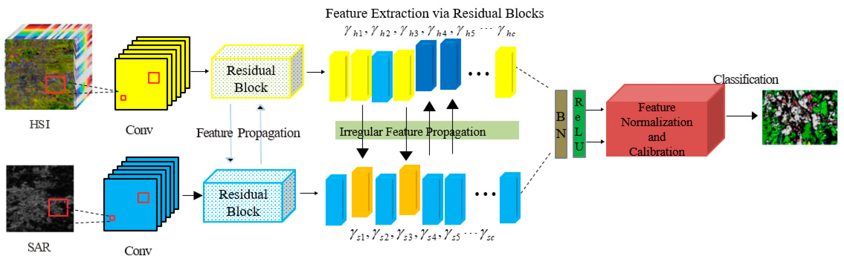
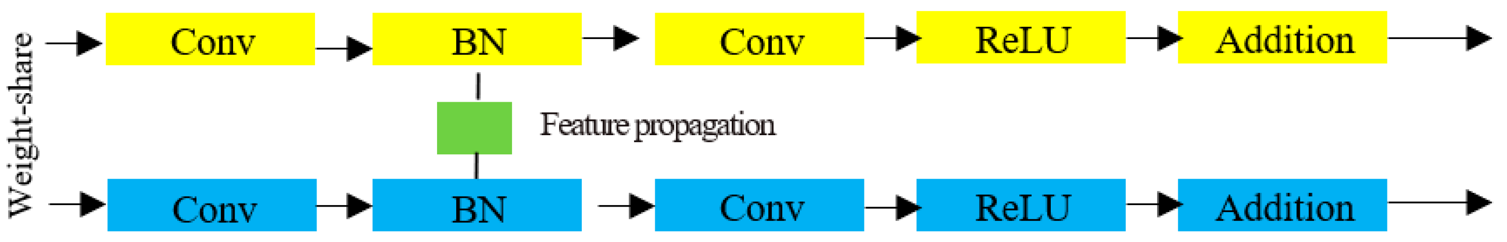
In this study, we propose a novel approach for classifying multimodal remote sensing data using irregular feature extraction. To enhance the model’s generalization capability, we employ weight-sharing residual blocks in a cascaded manner for feature extraction and adjust the number of parallel branches to facilitate collaborative processing without introducing extra parameters.

(2)

By privatizing the judgment factors within the BN layer, we effectively substitute redundant information in the channel. This enables us to fully leverage the complementary advantages of multimodal remote sensing data, while also imposing sparse constraints on specific judgment factors to mitigate any undesired feature propagation.

(3)

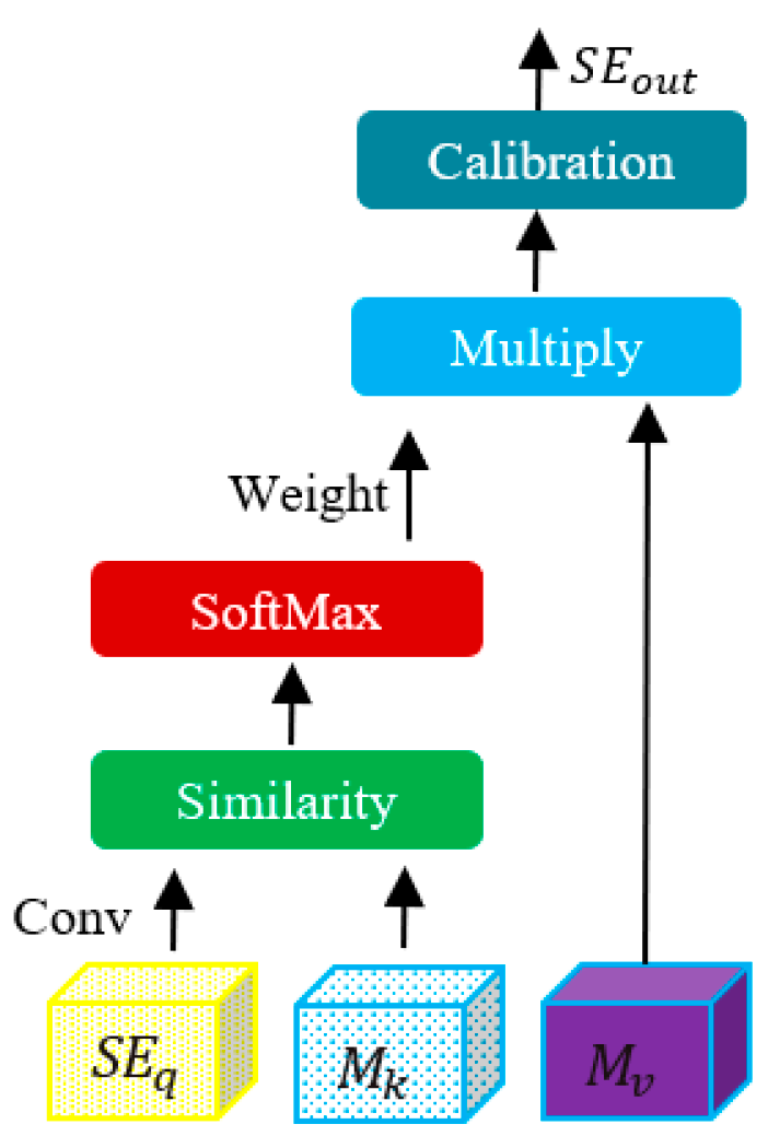
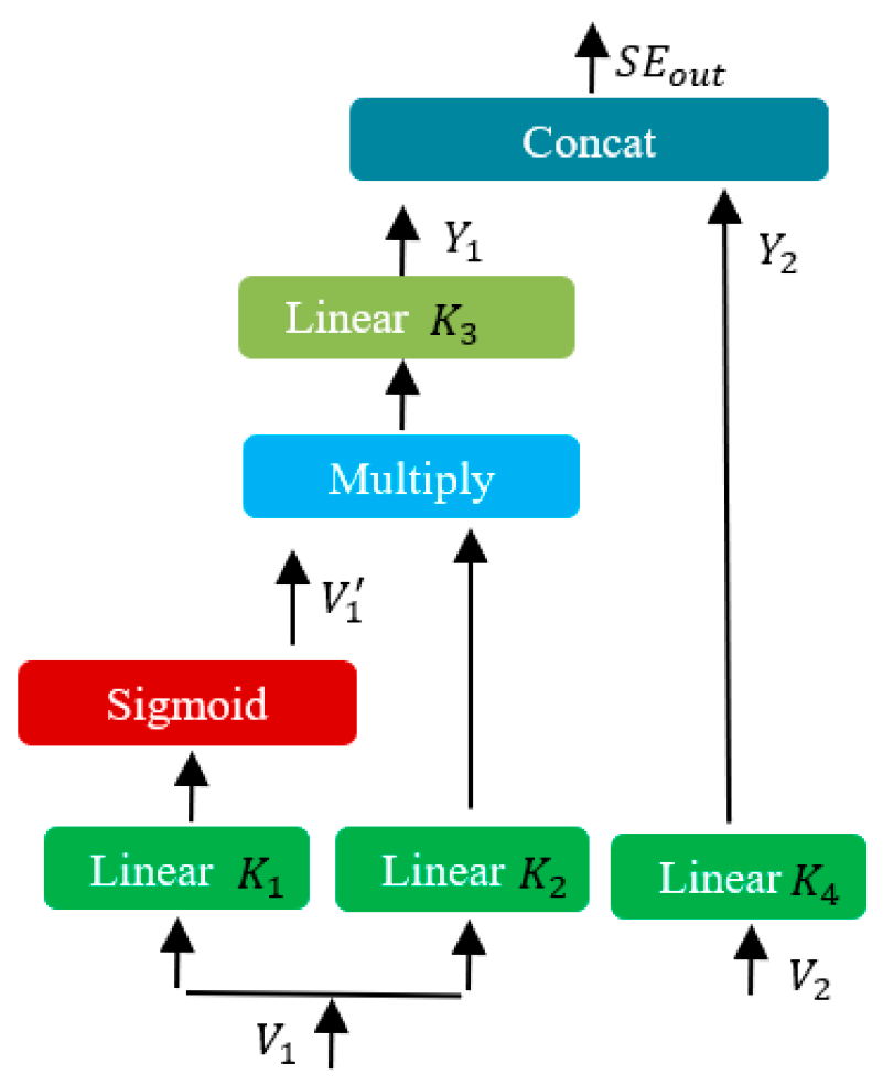
A module for normalizing and calibrating features was developed to enhance information integration, optimize spatial information discrimination, and minimize redundancy. The self-attention module underwent a calibration process as part of this enhancement.

2. Materials and Methods

The primary focus of this section lies in the network architecture of IFF-Net, specifically designed for the classification of multimodal remote sensing data. As illustrated in Figure 1, IFF-Net comprises three distinct modules: feature extraction via residual blocks, irregular feature propagation, and a feature normalization and calibration module. The extraction of features primarily relies on the utilization of residual blocks, which facilitate nonlinear feature propagation within redundant channels when the judgment factor of the BN layer falls below a predefined threshold value $\theta$. The data at position ${\gamma }_{hsic}$ are transmitted to the present channel when ${\gamma }_{hsic}<\theta$, where ${\gamma }_{hsic}$ represents the judgment factor of the c^th channel. Ultimately, the feature normalization and calibration module primarily aims to incorporate identifiable characteristics for feature classification.

2.1. Feature Extraction via Residual Blocks

The integration of spatial and spectral information from both HSI and SAR data is advantageous for classification purposes. To represent the center pixel, we utilize spatial neighborhood information of size r that has been pixelated. The HSI block is denoted as $X_h\in R^{r\times r\times c_h}$, while the SAR image block is denoted as $X_s\in R^{r\times r\times c_s}$, $c_h$ and $c_s$ refer to the corresponding channel quantities. The sub-network of the model comprises a CNN layer and multiple residual blocks, followed by a BN layer and an activation layer. To ensure compatibility with multimodal data, the initial CNN layer performs dimension matching without sharing weights. Common patterns are then extracted from the multimodal remote sensing data by weight-sharing residual blocks, which is central to the reorganization and integration of irregular features. The fusion of features is accomplished through the utilization of supplementary modules that are linked to the convolutional layer. Figure 2 illustrates the residual block for irregular feature propagation, where the optimization of BN parameters is conducted independently. Therefore, the determination of irregular feature propagation is based on comparing the judgment factor values of the private BN layer with a threshold value. By employing weight sharing, the two modalities’ features are endowed with a shared set of weights during feature extraction, effectively reducing the computational complexity from O(2r) to O(r). Simultaneously, the comparison between the judgment factor ${\gamma }_{hsic}$ and threshold $\theta$ in our model determines feature propagation across channels, leading to a space complexity reduction from O(2c) to O(c). This approach ensures that the model maintains its specificity. Thus, this approach reduces model complexity while preserving modal specificity. Unlike independent modal extraction, weight sharing of private BN layers can reduce the number of training parameters without compromising specificity. As a result, irregular feature fusion is considered an intriguing method for feature fusion research.

Additionally, the parameters are fine-tuned through the utilization of stochastic gradient descent (SGD) to optimize the loss function. The objective function can be formulated as

$$L=\rho (f\left(X_h,X_s\right),y)+\lambda {{\displaystyle \sum _{s=1}^S{\displaystyle \sum _{b=1}^B\left|{\gamma }_{hsic,l}\right|}}}_1$$

(1)

In the given equation, $\rho (\cdot )$ represents the cross-entropy loss between the output $f\left(X_h,X_s\right)$ and the actual label y. S denotes the number of input modes, B indicates the number of BN layers, and b denotes the b^th BN layer, l denotes the L1 norm. $\lambda$ is the regularization factor and regularization techniques are employed to eliminate invalid channels and enhance the generalization capability, thereby improving the overall robustness of the model. To impose sparse constraints on the partial judgment factor ${\gamma }_{hsic}$, L1 regularization is utilized. To demonstrate the preservation of network convergence in our proposed approach, Figure 2 showcases the residual block exhibiting irregular feature propagation. The theoretical derivation supporting this observation is presented below. The network’s convergence performance remains unaffected by irregular feature propagation. During training, we denote the output without irregular feature propagation as

$${\chi }_{l+1}=W_{l+1}{\chi }_l+b_{l+1}=W_{l+1}({\gamma }_{hsic}{\tilde{x}}_l+\alpha )+b_{l+1}$$

(2)

where $W_{l+1}$ and $b_{l+1}$ represent the weights and offsets of the next layer, respectively. ${\tilde{x}}_l$ is the input of the current layer, while ${\chi }_l$ is the output of the current layer, and $\alpha$ represents the offset of the current layer. Once ${\gamma }_{hsic}=0$, it means that the loss function is minimized and the output of the subsequent layer ${\chi }_{l+1}$ becomes a constant feature map ${\chi }_{l+1}=W_{l+1}\cdot \alpha +b_{l+1}$. With a similar definition, we denote the output of irregular feature propagation as follows:

$${\chi }_{l+1}^{\prime }=W_{l+1}^{\prime }{\chi }_l^{\prime }+b_{l+1}^{\prime }$$

(3)

where $b_{l+1}^{\prime }=W_{l+1}\cdot \alpha +b_{l+1}$, and ${W^{\prime }}_{l+1}$ represent the weights of the next layer. Since feature propagation occurs at ${\gamma }_{hsic}=0$, ${\chi }_{l+1}^{\prime }$ is always equal to ${\chi }_{l+1}$ when $W_{l+1}^{\prime }=0$, i.e., regardless of irregular feature propagation, the loss of the IFF-Net network always satisfies $L^{\prime }<=\min L$. As a result, the propagation of irregular features effectively eliminates superfluous data in multimodal datasets and enhances their suitability for training.

2.2. Irregular Feature Propagation

The deep neural network’s internal covariate bias leads to a decline in the performance of its hidden layer. The BN operation approximates the true distribution by means of a learnable judgment factor and offsets [35]. Specifically, this refers to data normalization, distribution scaling, and distribution offsets. The BN operation is

$$\eta ={\gamma }_{hsic}\tilde{x}+\alpha ={\gamma }_{hsic}\frac{x-\mu }{\sqrt{{\sigma }^2+\tau }}+\alpha$$

(4)

where $\mu$ represents the average value and $\sigma$ denotes the standard deviation of the input sample $x$. Additionally, $\eta$ is the output of the BN layer and $\tau$ is a constant that avoids division by zero. The symbol ${\gamma }_{hsic}$ signifies a judgment factor, $\tilde{x}$ is the output value normalized to the input $x$, and $\alpha$ represents the offset. Therefore, the derivative calculation can be performed on the input $x$, and the specific derivation process is as follows.

$$\begin{array}{ll}\frac{\partial L}{\partial x}& =\frac{\partial L}{\partial \tilde{x}}\frac{\partial \tilde{x}}{\partial x}+\frac{\partial L}{\partial \sigma }\frac{\partial \sigma }{\partial x}+\frac{\partial L}{\partial \mu }\frac{\partial \mu }{\partial x}\\ & =\frac{\partial L}{\partial \eta }\frac{\partial \eta }{\partial \tilde{x}}\cdot \left(\frac{\partial \tilde{x}}{\partial \mu }\frac{\partial \mu }{\partial x}+\frac{\partial \tilde{x}}{\partial \sigma }\frac{\partial \sigma }{\partial x}+\frac{\partial \tilde{x}}{\partial x}\right)\\ & =\frac{\partial L}{\partial \eta }\cdot {\gamma }_{hsic}\cdot \left(\frac{\partial \tilde{x}}{\partial \mu }\frac{\partial \mu }{\partial x}+\frac{\partial \tilde{x}}{\partial \sigma }\frac{\partial \sigma }{\partial x}+\frac{\partial \tilde{x}}{\partial x}\right)\end{array}$$

(5)

It can be seen from Equation (5) that the transmission of irregular features is determined by the judgment factor. When ${\gamma }_{hsic}\to 0$, the gradient value of $\frac{\partial L}{\partial x}$ is close to zero. The influence of x on the subsequent classification task is negligible. It is challenging to alter this condition during the deep learning process. In other words, in backpropagation, we first calculate the judgment factor using its corresponding formula.

$$\frac{\partial L}{\partial {\gamma }_{hsic}}=\frac{\partial L}{\partial \eta }\frac{\partial \eta }{\partial {\gamma }_{hsic}}\pm \lambda =\{\begin{array}{c}\frac{\partial L}{\partial \eta }\tilde{x}+\lambda ,if{\gamma }_{hsic}>0\\ \frac{\partial L}{\partial \eta }\tilde{x}-\lambda ,if{\gamma }_{hsic}<0\end{array}$$

(6)

where $\tilde{x}=({(x-\mu )/({\sigma }^2+\tau )}^{1/2})$, $L$ denotes the loss function, which is defined in Equation (1), and ${\gamma }_{hsic}=0$ denotes the local minima during training. In other words , when ${\gamma }_{hsic}=0$, $(\partial L/\partial \eta )\tilde{x}+\lambda >0$, and $(\partial L/\partial \eta )\tilde{x}-\lambda <0$, $\tilde{x}$ acts as a standard Gaussian random variable. The sample X satisfies the standard normal distribution function, i.e., X~N(0,1), whose data equation is expressed as

$$\psi (x)=\frac{1}{\sqrt{2\pi }}{\displaystyle {\int }_{-\infty }^x{e}^{-\frac{t^2}{2}}}dt$$

(7)

Therefore, the standard Gaussian probability is calculated as

$$\begin{array}{ll}P& =\frac{1}{\sqrt{2\pi }}{\displaystyle {\int }_{-\lambda {\left|\frac{\partial L}{\partial \eta }\right|}^{-1}}^{\lambda {\left|\frac{\partial L}{\partial \eta }\right|}^{-1}}{e}^{-\frac{t^2}{2}}}dt=\frac{1}{\sqrt{2\pi }}{\displaystyle {\int }_{-\infty }^{\lambda {\left|\frac{\partial L}{\partial \eta }\right|}^{-1}}{e}^{-\frac{t^2}{2}}}dt-\frac{1}{\sqrt{2\pi }}{\displaystyle {\int }_{-\infty }^{-\lambda {\left|\frac{\partial L}{\partial \eta }\right|}^{-1}}{e}^{-\frac{t^2}{2}}}dt\\ & =\psi (\lambda {\left|\frac{\partial L}{\partial \eta }\right|}^{-1})-\psi (-\lambda {\left|\frac{\partial L}{\partial \eta }\right|}^{-1})\end{array}$$

(8)

Because of the symmetry of the normal, Equation (8) can be expressed as

$$\begin{array}{ll}P& =\psi (\lambda {\left|\frac{\partial L}{\partial \eta }\right|}^{-1})-(1-\psi (\lambda {\left|\frac{\partial L}{\partial \eta }\right|}^{-1}))\\ & =2\psi (\lambda {\left|\frac{\partial L}{\partial \eta }\right|}^{-1})-1\end{array}$$

(9)

In fact, $\partial L/\partial \eta$ always converges to 0 at the convergence point, Consequently, $-\lambda {(\partial L/\partial \eta )}^{-1}\to -\infty$ and $\lambda {(\partial L/\partial \eta )}^{-1}\to +\infty$. The standard Gaussian random variable $\tilde{x}$ has a probability $P$ that approaches unity. To put it simply, ${\gamma }_{hsic}=0$ indicates that there exists redundancy in the present channel. During subsequent training stages, there will be an increased likelihood $P$ for this redundancy in current channel information to occur. Consequently, the incorporation of feature fusion confers advantages in eliminating such redundancies and enhancing learning processes. Additionally, maintaining ${\gamma }_{hsic}$ near 0 allows irregular feature propagation, which aids in extracting complementary details from diverse remote sensing data modalities. From this point forward, by employing feature fusion when ${\gamma }_{hsic}\to 0$, we effectively eliminate data redundancies. This calculation for performing feature fusion can be represented as follows:

$${\delta }_{h,c}=\{\begin{array}{l}{\gamma }_{hsic,h,c}\frac{x_{h,c}-{\mu }_{h,c}}{\sqrt{{\sigma }_{h,c^2}+\tau }}+{\alpha }_{h,c},if{\gamma }_{hsic,h,c}>\theta \\ {\gamma }_{hsic,s,c}\frac{x_{s,c}-{\mu }_{s,c}}{\sqrt{{\sigma }_{s,c^2}+\tau }}+{\alpha }_{s,c},otherwise\end{array}$$

(10)

In the HSI branch, h, c represents the BN parameter of the c^th channel, while in the SAR branch, s, c represents the BN parameter of the c^th channel. The feature $x_{h,c}$ corresponds to the c^th channel in $X_h$, and $x_{s,c}$ corresponds to the c^th channel in $X_s$. Here, a threshold value $\theta =2\times {10}^{-3}$ is used close to 0. If ${\gamma }_{hsic,h,c}<\theta$, it indicates that the current feature of the c^th channel is redundant and should be replaced by another channel. This means that when a particular channel no longer contributes to subsequent predictions, it is substituted with feature propagation from a corresponding modality’s channel. Applying regularization to the judgment factor ${\gamma }_{hsic}$ can effectively extract the complementary information between modes and reduce the propagation of invalid irregular features.

2.3. Feature Normalization and Calibration

Reaching complementary benefits is made possible through complete information exchange among multimodal remote sensing data after the propagation of irregular features. Prior to classification, it is necessary to standardize and calibrate the multimodal remote sensing data features. To enhance the capabilities of feature recognition, we propose incorporating a module for feature normalization and calibration that establishes associations between global and local features and identifiable characteristics; Enhancing feature normalization and calibration via an enhanced self-attention mechanism. Refer to Figure 3 for an illustration of the feature normalization and calibration module. The improved self-attentive feature can be represented as $SE\left(Q,K,V\right)$, which conducts query, key, and value operations on its $Q,K,V\in R^{N\times C}$. In this case, $N=H\times W$ represents the dimensions of a given area with height H multiplied by width W, while C signifies the quantity of channels. Initially, we calculate the similarity between Q and K, before determining a weighted average vector across V based on these similarity scores. Consequently, we can express this overall improved self-attention equation in a generalized form.

$$c_{i,j}=soft\max \left(m_i{k}_j^T\right)$$

(11)

$${\tilde{v}}_i={\displaystyle \sum _j{c}_{i,j}{v}_j}$$

(12)

In the given equation, $m_i\in R^{1\times C}$ represents the i^th query Q, $k_j\in K$, and $v_j\in V$ denote the j^th set of keys and values, respectively, $c_{i,j}$ refers to the similarity score between $m_i$ and $k_j$, while ${\tilde{v}}_i\in \widehat{V}$ stands for the attention vector of $m_i$.

Obviously, Q, K, and V are commonly linear transformations of the input features $S{E}_q$. Hence, the improved self-attention mechanism solely focuses on the elemental relations within a single sample while disregarding the relationships among different samples. In this study, we propose an enhanced feature normalization and calibration module that incorporates a calibration module integrated with an improved self-attention module. The improved self-attention module employs a dataset consisting of two sets of self-learning parameters instead of (K, V) key–value pairs. These two datasets are used to store the relationships between data elements throughout the training process. For example, $S{E}_q$ denotes an output value after the propagation of an irregular feature Q in the improved self-attention mechanism, which is then fed into the feature normalization and calibration module. The mathematical formula for this is

$$c_{i,j}^{\prime }=\mathrm{softmax}\left(norm(m_i{g_k^j}^T)\right)$$

(13)

$${\tilde{v}}_{i,j}^{\prime }={\displaystyle \sum _j{c}_{i,j}^{\prime }{g}_v^j}$$

(14)

In this model, we utilize two datasets, $M_k\in R^{M\times C}$ and $M_v\in R^{M\times C}$, which are linear learning parameters. These datasets contain rows $M_k$ and $M_v$, respectively, where $c_{i,j}^{\prime }$ represents the similarity score between $m_i$ and $g_k^j$. The size of the convolutional kernel is denoted by M. By sharing parameters across the training set, these storage units improve regularization effects while reducing learned parameters and linear complexity when M < N. Both the self-attention and improved self-attention module outputs are weighted averages for each query. To address this issue, a normalization and calibration module is added on top of the global attention module, as shown in Figure 4, to ensure accurate results.

First, the linear layer averages the output characteristics of the improved self-attention module into two parts $[V_1,V_2]$, and then, defines four convolution kernels $[K_1,K_2,K_3,K_4]$, which have the shape $[C/2,C/2,k,k]$. Specifically, $[K_1,K_2,K_3]$ are used for feature calibration, which is calculated as

$$V_1^{\prime }=\sigma (UP[(AvgPool(V_1)\ast K_1])$$

(15)

$$Y_1=((V_1\ast K_2)\cdot V_1^{\prime })\ast K_3$$

(16)

where $AvgPool(\cdot )$ is an average pooling operation with a convolution kernel of $2\times 2$ and a step size of 2. $UP(\cdot )$ refers to the utilization of bilinear interpolation for increasing the resolution to match the initial assessment. In this context, $\ast$ denotes the convolution operation while $\sigma$ represents the sigmoid function. By employing feature calibration, it becomes possible to acquire more distinct local spatial regions. Moreover, the vector $K_4$ is used to maintain the original spatial texture structure without any calibration operation, i.e., $Y_2=V_2\ast K_4$. $Y_1$ and $Y_2$ perform the join operation to output the results after feature normalization and calibration, calculated as

$$S{E}_{out}=concat(Y_1,Y_2)$$

(17)

Ultimately, pixelated summation fusion is employed to classify the normalization and calibration features of each mode.

3. Results

3.1. Data Description

(1) Augsburg dataset: This dataset describes the land cover around Augsburg, Germany, and consists of remotely sensed images acquired by two different remote sensing instruments, namely, satellite-based HSI and polarized synthetic-aperture radar (PolSAR) images. The HSI data were acquired using the HySpex sensor, while the PolSAR images were obtained from the sentinel-1 sensor. The spatial resolution of all images in the Augsburg dataset is ground sampling distance (GSD) to a uniform resolution of 30 m to facilitate multimodal data fusion. Specifically, the Augsburg dataset has a spatial size of 332 × 485 pixels, where the HSI consists of 180 spectral bands in the range of 0.4~2.5 μm and the SAR consists of four polarization decomposition features (The elements VV-VH, which correspond to the off-diagonal components of the polarized synthetic aperture radar (SAR) covariance matrix, represent the real and imaginary parts respectively). Ground truth maps for the Augsburg dataset were provided by M. Haklay et al. [36] and hand-labeled by experts with extensive knowledge of fieldwork and photo interpretation.

The Augsburg dataset is publicly and freely available from Hu et al. [37]. The data can be downloaded from the website: https://mediatum.ub.tum.de/1657312 (accessed on 30 January 2024).

Table 1. Describes the sizes of training and test sets for the Augsburg dataset.

Class No	Class Name	Training Set	Testing Set
C1	Forest	2026	11,481
C2	Residential Area	4549	25,780
C3	Industrial Area	578	3273
C4	Low Plants	4029	22,828
C5	Allotment	86	489
C6	Commercial Area	247	1398
C7	Water	230	1300
	Total	11,745	66,549

provides information on the categories involved in the scenarios as well as the sizes of both training and test sets.

(2) Berlin dataset: The dataset provides a comprehensive description of Berlin city and its rural periphery. The first data are synthesized simulated EnMAP data based on HyMap HS data. The second data are from the Sentinel-1 dual polarization (VV-VH) single look complex (SLC) product, downloaded from the European Space Agency. Specifically, the HSI spatial resolution is GSD to 30 m, and the HyMap hyperspectral sensor records wavelengths ranging from 400 to 2500 nm, 244 spectral bands, and a spatial size of 797 × 220 pixels. The spatial resolution of the SAR image is GSD to 13.89 m, the spatial size is 1723 × 476 pixels, and four dual-polarized bands (VV-VH) are used. The SAR data are fed into a pre-processing pipeline based on the SNAP toolbox downloaded from ESA, including orbit correction, radiometric correction, and speckle reduction. The algorithm of nearest neighbor interpolation is used on the HSIs to match the spatial size of the SAR images. Additionally, M. Haklay et al. [36] provide ground truth maps and expert-labeled sample data.

Table 2. Describes the sizes of training and test sets for the Berlin dataset.

Class No	Class Name	Training Set	Testing Set
C1	Forest	8243	46,711
C2	Residential Area	40,296	228,346
C3	Industrial Area	2935	16,631
C4	Low Plants	8887	50,368
C5	Soil	2614	14,812
C6	Allotment	1996	11,309
C7	Commercial Area	3724	21,100
C8	Water	1001	5671
	Total	69,696	394,948

lists the categories of the dataset, the training data, and the test data. The Berlin dataset is publicly and freely available from D. Hong et al. [38]. The data can be downloaded from the following website: http://doi.org/10.5880/enmap.2016.002 (accessed on 25 February 2024).

3.2. Experimental Setup

(1) Evaluation metrics: In this study, we assess the performance of a classifier for multimodal remote sensing data using three commonly employed metrics: overall accuracy (OA), average accuracy (AA), and kappa coefficient (κ). Generally, higher values of these metrics indicate better performance in classifying remote sensing images. OA, AA, and κ provide quantitative evaluations of classification performance, with their respective formulas as follows:

$$OA=\frac{N_c}{N_a}$$

(18)

$$AA=\frac{1}{C}{\displaystyle \sum _{i=1}^C\frac{N_c^i}{N_a^i}}$$

(19)

and

$$\kappa =\frac{OA-P_e}{1-P_e}$$

(20)

In this context, $N_c$ represents the count of accurately classified instances, $N_a$ represents the total count of instances, $N_c^i$ signifies the count of instances belonging to a specific category i within those that are accurately classified, and $N_a^i$ indicates how many instances belong to category i out of all instances. Within $\kappa$, $P_e$ refers to an anticipated prior probability, which can be computed by

$$P_e=\frac{N_r^1\times N_p^1+\dots N_r^i\times N_p^i+\cdots +N_r^C\times N_p^C}{N_a\times N_a}$$

(21)

where $N_r^i$ denotes the number of true samples for each category and $N_p^i$ denotes the number of predicted samples for each category.

(2) Implementation details: The IFF-Net model experiments proposed in this paper are implemented on the TensorFlow 2.0 platform, and the libraries used for model computation are CUDA10.0 and CuDNN10.0, using a Dell tower server, which the server is branded Dell and purchased from Luzhou, Sichuan, China, with Inter Xeon Silver 4210 2.60 GHz CPU, 128 GB of RAM, and a GPU of NVIDIA GeForce GTX 3080Ti. In this paper, the square field for $r\times r$ represents the spatial information of the center pixel, due to the rich spatial information fused with multimodal information the performance of IFF-Net on small image blocks has a great advantage compared to that of larger image blocks. Through experimental comparative analysis, the experimental parameter in this paper set the block size to r = 12. Regarding the regularization factor $\lambda$, which is used to balance the weights between the two loss values, the loss function in this paper is defined in Formula (1), and the $L_1$ paradigm acts on the judgment factor to achieve the sparsity constraint. A larger $\lambda$ degrades the classification performance, and the performance starts to decay when $\lambda$ approaches 0. When $\lambda$ > 0.1, the classification performance drops on both datasets. The experimental results show that $\lambda$ = 0.05 is chosen as the regularization factor for the IFF-Net network. Empirically, an appropriate increase in the number of convolutional layers can enhance classification performance and accuracy; however, it incurs a higher computational cost and leads to a slower network convergence speed. In the case of insufficient training samples, it can easily lead to overfitting. At the same time, a larger n will lead to an increase in the use of random-access memory (RAM) for the model parameters during training. Meanwhile, a larger n value will also lead to a decrease in the OA value. The selection of two residual blocks with feature extraction and propagation, where $n$ = 2, is made after comprehensive consideration. The running times of the classification methods employed in this study on the experimental dataset are presented in

Table 3. Running times on the experimental datasets.

Classification Method	Time(s) on Berlin	Time(s) on Augsburg
SVM	276.21	256.51
CapsNet	280.26	262.36
S2FL	157.18	121.68
LeMA	164.12	152.32
Two-branch CNN	371.42	312.12
IFF-Net	421.65	361.25

.

The proposed IFF-Net network in the paper primarily accomplishes feature extraction, propagation, and calibration for multimodal remote sensing images without the need for manual tuning or parameter setting. To ensure a fair comparison with other network architectures, the designed IFF-Net structure in this study closely resembles existing network structures while maintaining similar parameters and complexity.

Hyperparametric analysis of the image block size r: A specific comparison of the image block sizes r and OA of the two datasets is performed. The $r\times r$ square neighborhood represents the spatial information of the central pixel, $r=\left[5,7,9,12,13,15\right]$. As can be seen from

Table 4. Comparison of OA and image block size.

r	Berlin (OA%)	Augsburg (OA%)
5	68.21	88.36
7	68.86	88.58
9	69.85	88.96
12	71.02	90.52
13	69.92	86.42
15	68.91	86.06

, r is positively correlated with OA in most cases. When the image block size r is large enough, the improvement in OA is insignificant. As the spatial information is improved by multimodal information fusion, the performance of a small block of images is more satisfactory for the IFF-Net method. Through comprehensive comparison and analysis, it can be seen through the above Table 4 that a more satisfactory performance can be obtained by using r = 12 for the Berlin dataset and Augsburg dataset. Therefore, a larger patch size can reduce the interference of mixed boundaries, but for urban land cover classification the feature boundaries are clear and continuously distributed. Larger image patch sizes are prone to artefacts and increase computational burden

Hyperparametric analysis of the number of residual blocks n: Based on experience, it is known that more convolutional layers need to fit more parameters and are beneficial to image classification, where overfitting can easily occur in the case of insufficient training samples. From

Table 5. Comparison of OA and residual blocks.

n	Berlin (OA%)	Augsburg (OA%)
1	67.31	88.46
2	71.02	90.52
3	68.84	89.25
4	69.10	89.32
5	66.79	87.43

, it can be seen that when the number of residual blocks n > 2, the OA value gradually decreases. When n = 1, the IFF-Net method displays underfitting, which affects the classification performance. Therefore, the IFF-Net method proposed here chooses n = 2 as the hyperparameter of residual blocks.

The loss function of the proposed method is defined as presented in Equation (1), and its utilization aids in regularization optimization. In this study, the L1 norm is employed to impose sparsity constraints on certain judgment factors. $\lambda$ represents a regularization factor that effectively balances the weights between the two loss measures.

Table 6. The relationship between OA and the regularization factor $\lambda$ is described.

λ	Berlin (OA%)	Augsburg (OA%)
1	65.71	88.96
0.5	68.86	88.48
0.1	69.44	89.73
0.05	71.02	90.52
0.01	69.59	90.16

illustrates the correlation between different values of $\lambda$ and OA. Notably, when $\lambda =0.05$, the IFF-Net model introduced here demonstrates superior performance on both datasets. Conversely, for larger values of $\lambda >0.1$, an increased value leads to a degradation in focus within the classification component. Consequently, based on our findings, we select $\lambda =0.05$ as the optimal regularization factor for IFF-Net.

(3) Comparison with state-of-the-art multimodal algorithms: To assess the classification effectiveness of the IFF-Net network proposed in this study, we compare it quantitatively and qualitatively with several advanced algorithms for multichannel remote sensing data classification. These algorithms include support vector machine (SVM) [39], CapsNet [40], S2FL [25], LeMA [21], and Two-branch CNN [26].

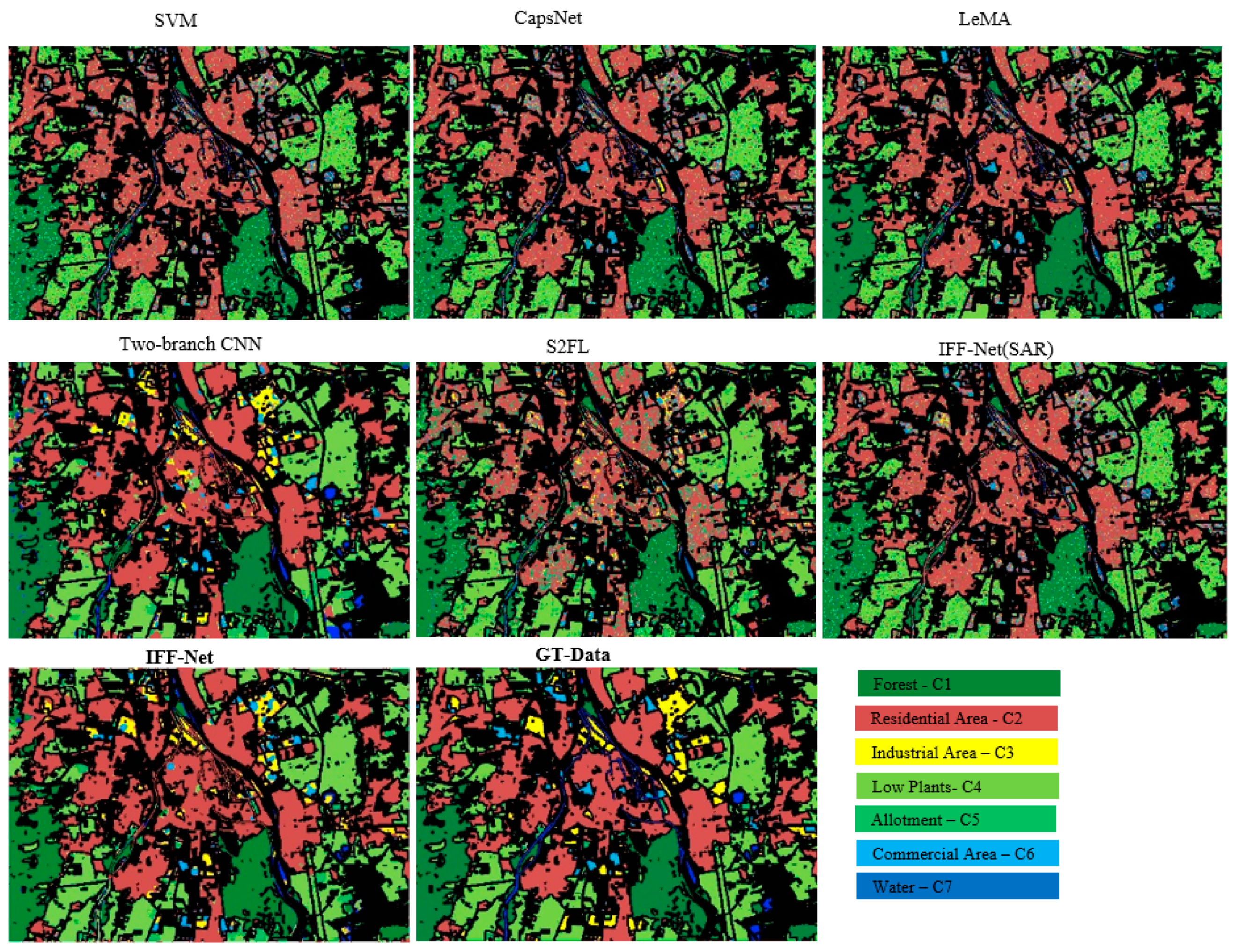
3.3. Results and Analysis on Augsburg Data

(1) Quantitative comparison:

Table 7. Quantitative comparison of different methods in terms of OA, AA, and κ on the Augsburg dataset.

Class No	SVM (HSI)	SVM (SAR)	SVM (HIS + SAR)	LeMA (HIS + SAR)	CapsNet (HIS + SAR)	Two-Branch CNN (HIS + SAR)	S2FL (HIS + SAR)	IFF-Net (SAR)	IFF-Net (HIS + SAR)
C1	82.01 ± 01.04	83.23 ± 01.35	90.33 ± 01.26	86.86 ± 02.05	85.10 ± 00.85	93.76 ± 00.61	88.80 ± 01.11	84.25 ± 00.84	98.21 ± 00.31
C2	86.24 ± 01.44	85.51 ± 01.46	90.47 ± 01.31	90.08 ± 01.85	89.02 ± 01.25	94.19 ± 00.44	89.36 ± 01.25	86.36 ± 01.37	97.23 ± 00.46
C3	21.97 ± 00.84	5.20 ± 00.76	20.37 ± 01.12	42.00 ± 02.26	40.44 ± 01.16	58.73 ± 01.21	45.90 ± 00.61	17.64 ± 00.81	50.95 ± 00.38
C4	80.81 ± 01.42	67.98 ± 01.04	84.57 ± 00.64	86.79 ± 01.56	85.35 ± 00.44	85.51 ± 00.67	87.53 ± 00.53	91.31 ± 00.45	91.63 ± 01.21
C5	36.63 ± 02.08	5.42 ± 00.37	36.71 ± 00.55	47.34 ± 01.04	45.00 ± 01.31	51.86 ± 00.72	68.64 ± 00.61	30.15 ± 01.23	83.36 ± 00.35
C6	11.72 ± 00.86	1.14 ± 01.08	9.58 ± 00.29	23.30 ± 00.87	21.80 ± 00.21	28.35 ± 00.53	10.97 ± 01.36	12.64 ± 00.14	38.35 ± 00.72
C7	45.12 ± 01.21	12.60 ± 01.35	45.65 ± 00.72	46.99 ± 01.16	45.38 ± 02.05	49.37 ± 01.05	47.65 ± 00.44	14.85 ± 00.36	28.51 ± 00.44
OA (%)	81.20 ± 00.76	79.63 ± 00.54	82.01 ± 01.04	83.49 ± 01.34	82.12 ± 00.52	86.83 ± 00.71	83.86 ± 00.29	80.98 ± 00.52	90.52 ± 00.38
AA (%)	53.50 ± 01.32	40.73 ± 01.13	53.95 ± 01.61	60.48 ± 01.51	58.87 ± 00.64	65.97 ± 00.66	62.40 ± 00.37	48.17 ± 00.29	69.74 ± 00.27
κ	74.53 ± 00.87	72.41 ± 00.46	73.74 ± 00.62	77.54 ± 01.32	75.80 ± 00.38	81.91 ± 00.59	78.03 ± 00.49	74.19 ± 00.63	86.74 ± 00.67

presents the quantitative outcomes of various multimodal techniques on three widely employed metrics, namely, OA, AA, and κ. In general, the classification accuracy of the deep-learning-based classification methods is better than that of other methods, such as Two-branch CNN and the IFF-Net method proposed in this paper. The classification accuracy of multimodal data fusion is to some extent higher than that of single-modal data, e.g., the classification accuracy of support vector machine (SVM) classifiers is slightly higher for HSI + SAR for the individual analysis of HSI or SAR. The classification accuracies achieved by traditional subspace and morphological methods exhibit a slight superiority over those obtained through SVM and CapsNet approaches with simple data overlays. Among the semi-supervised methods, the LeMA method fully considers both labeled and unlabeled samples, maps different modalities of the data through a common subspace, and achieves higher classification accuracy, with more than 1% improvement in OA compared to SVM classifiers. The OA value is enhanced by a minimum of 1.6% through the utilization of deep-learning-based classification methods, including Two-branch CNN and the proposed IFF-Net method. Based on the experimental results presented in Table 4, it is evident that SVM exhibits a tendency to generate numerous noise regions by simply stacking the data, resulting in slightly inferior classification accuracy methods. The CapsNet method employs feature stacking in the feature fusion stage; however, it fails to fully integrate the spatial and spectral information. Consequently, the classification OA value closely resembles that of SVM and LeMA with minimal disparity. Two-branch CNN and IFF-Net excel at extracting highly distinctive feature representations and effectively capturing the inherent correlations among diverse modalities. This leads to better classification results using IFF-Net and Two-branch CNN. The OA of the S2FL method is better than the CapsNet method, but the classification accuracy of the single category is not outstanding. The OA of Two-branch CNN is better than those of the S2FL and CapsNet methods, and it has the highest accuracy and the best performance on category C3 and category C7. The well-designed feature fusion module improves the discrimination of the fused information. Compared with other methods, the OA value of the IFF-Net method proposed in this paper is increased by +8.51%, +7.03%, +8.40%, +3.69%, and 6.66%, respectively. Among them, the IFF-Net method achieves significant performance on categories C1, C2, C4, C5, and C6, while C3 is slightly inferior to the Two-branch CNN. The OA of C7 is not superior to other methods due to the small training sample size and the influence of noise in feature fusion, and the overall results also maintain an important quantitative gain compared with other methods. The IFF-Net method proposed in this paper outperforms other classification methods in multimodal remote sensing data classification and achieves better classification accuracy. In order to evaluate the stability and robustness of the proposed IFF-Net method, 10 experiments are performed on the test sample data, and the standard deviations of each of the categories are calculated for statistical evaluation.

(2) Visual comparison: The classification graph for the Augsburg dataset is shown in Figure 5. GT-Data is the real ground classification map. the SVM classifier considers less spatial information, the classification map is noisy, and the classification effect is not good; especially for the industrial area (C3) and commercial area (C6), a large number of misclassifications pollute the map. The CapsNet and S2FL classifiers have noise in the classification of the commercial area (C6), which affects the classification effect. Compared with the SVM classifier, the CapsNet and S2FL classifiers have better classification effects for the industrial area (C3) and commercial area (C6). In addition, the method based on deep learning performs well on the overall classification effect, and the classification map is clearer. The Two-branch CNN classifier is better than other classifiers and the classification map is smoother and less noisy, particularly with regards to the delineation of boundaries between vegetation (C1 and C4) and C7 bodies. The proposed IFF-Net classifier fully integrates spectral and spatial information, and achieves the best classification results, especially for forest (C1), industrial area (C2), and low vegetation (C4), which are close to the real scenes. In addition, the classification effect of SAR remote sensing data by the proposed IFF-Net classifier alone is noisy, and the classification effect is not good, especially for the commercial area (C6) and water (C7). Through intuitive comparative analysis, the classification map generated by the proposed IFF-Net can provide more realistic land cover, and the classification effect performs the best.

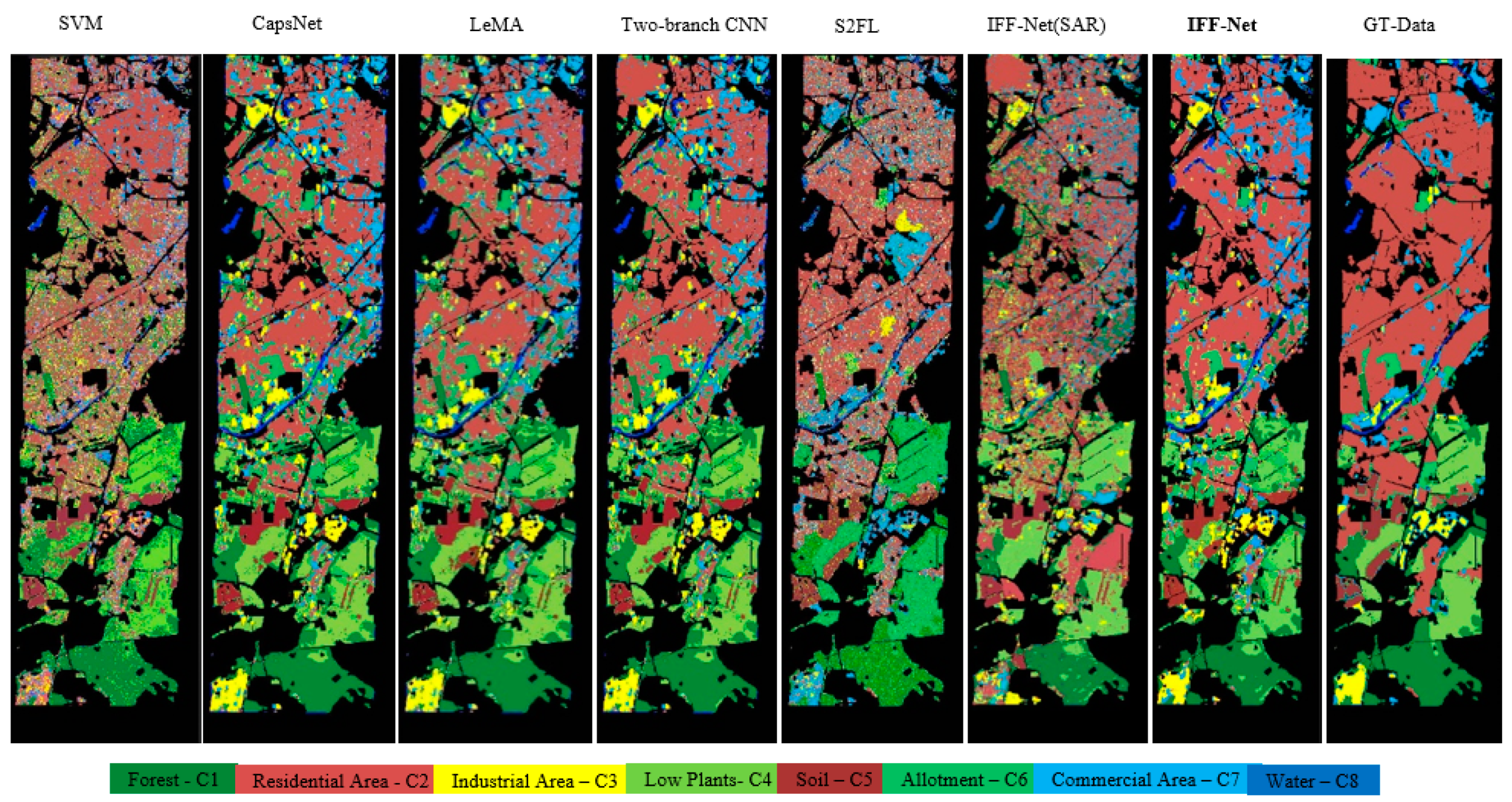
3.4. Results and Analysis on Berlin Data

(1) Quantitative comparison: From the experimental results listed in

Table 8. Quantitative comparison of different methods in terms of OA, AA, and κ on the Berlin dataset.

Class No	SVM (HSI)	SVM (SAR)	SVM (HSI + SAR)	CapsNet (HSI + SAR)	LeMA (HSI + SAR)	Two-Branch CNN (HSI + SAR)	S2FL (HSI + SAR)	IFF-NET (SAR)	IFF-Net (HSI + SAR)
C1	72.57 ± 00.68	31.33 ± 01.04	68.11 ± 01.21	84.86 ± 01.27	84.11 ± 00.84	85.09 ± 00.75	79.52 ± 01.44	40.12 ± 00.98	82.59 ± 00.54
C2	41.93 ± 01.24	28.52 ± 01.42	62.22 ± 00.65	65.22 ± 00.43	64.84 ± 01.53	68.48 ± 00.44	49.41 ± 02.15	61.21 ± 01.34	64.53 ± 00.72
C3	37.72 ± 01.13	35.60 ± 02.11	29.01 ± 01.26	48.32 ± 00.51	42.53 ± 00.76	48.09 ± 00.39	45.18 ± 01.31	11.43 ± 00.76	60.12 ± 00.36
C4	68.23 ± 02.06	43.07 ± 00.72	78.93 ± 00.58	80.70 ± 01.23	80.04 ± 01.27	78.43 ± 01.27	70.50 ± 02.17	46.28 ± 00.58	81.88 ± 00.59
C5	80.01 ± 00.44	51.00 ± 00.36	80.99 ± 01.34	69.08 ± 00.49	80.66 ± 00.69	80.25 ± 00.65	81.47 ± 00.75	45.03 ± 00.68	82.48 ± 00.67
C6	61.89 ± 00.54	32.27 ± 00.81	44.12 ± 00.72	55.08 ± 01.24	54.07 ± 01.47	48.70 ± 00.61	61.31 ± 00.81	7.24 ± 00.43	71.26 ± 01.13
C7	35.84 ± 00.36	12.03 ± 01.06	31.75 ± 00.68	26.11 ± 00.61	27.40 ± 00.58	25.16 ± 02.16	29.63 ± 00.45	14.85 ± 00.62	48.61 ± 00.34
C8	66.13 ± 01.27	33.78 ± 00.82	66.06 ± 01.41	59.59 ± 00.78	57.75 ± 02.06	58.52 ± 00.17	57.24 ± 01.21	34.64 ± 00.37	70.71 ± 00.29
OA (%)	51.11 ± 01.12	31.56 ± 01.10	63.25 ± 00.68	67.05 ± 01.12	66.21 ± 01.26	67.45 ± 00.48	56.06 ± 01.13	49.80 ± 00.75	71.02 ± 00.38
AA (%)	58.04 ± 00.93	33.45 ± 00.87	57.65 ± 00.73	61.12 ± 00.87	62.05 ± 01.13	61.59 ± 00.57	59.28 ± 01.25	32.60 ± 00.67	70.27 ± 00.29
κ	37.38 ± 00.75	25.60 ± 01.12	48.62 ± 00.44	52.07 ± 01.08	52.12 ± 01.21	54.36 ± 00.72	42.46 ± 00.87	36.18 ± 00.53	70.03 ± 00.51

, it is evident that multimodal remote sensing feature fusion can improve classification accuracy. The classification accuracy of the classifier using HSIs or SAR images alone is less than that of the classifier using HSI and SAR fusion. We speculate that the simple data superposition fusion method cannot eliminate the noise and makes the classification effect of SAR images worse. Fusion of spatial and spectral information facilitates image interpretation. As can be seen from Table 8, the classification accuracy of deep-learning-based classifiers is better, and the CapsNet classifier outperforms the traditional SVM classifier, S2FL classifier, and LeMA classifier in terms of classification performance. The OA of Two-branch CNN is improved, which is slightly better than that of the CapsNet classifier, especially in the classification accuracy of C1 and C2. Compared with other classifiers, the OA of the IFF-Net classifier proposed in this paper is increased by +7.77%, +3.97%, +4.81%, +3.57%, and 14.96%, respectively. Among them, the IFF-Net classification method achieves the best classification accuracy on single classes C3, C4, C5, C6, C7, and C8. Overall, the IFF-Net method proposed in this paper has the best classification accuracy compared with other methods. It makes the feature information fully fused by the irregular feature fusion strategy, which improves the classification accuracy. In order to evaluate the stability and robustness of the proposed IFF-Net method, 10 experiments are performed on the test sample data, and the standard deviations of each of the categories are calculated for statistical evaluation.

(2) Visual comparison: Figure 6 shows the classification effect of the proposed method in this paper and the comparison method on the Berlin dataset, where GT-Data is the real ground classification map. It can be seen that there is noise on top of the classification maps of the SVM method and S2FL method, which affects the classification effect. In particular, the S2FL classification method classifies part of the residential area (C2) as commercial (C7) or industrial (C3), which is not consistent with the real features. The classification method based on deep learning, the Two-branch CNN classifier, and the proposed IFF-Net classifier have better classification results. The overall classification effect of the Two-branch CNN classifier is better than the CapsNet classifier, especially for the classification effect of residential area (C2) and forest (C1). The IFF-Net classifier proposed in this paper fully integrates spectral and spatial information, and has the best classification effect. Especially, the classification effect of low plants (C4) and allotment (C5) is more consistent with the real scenes, and the effect is better than other classification methods. Therefore, through intuitive comparative analysis, the classification effect map generated by the IFF-Net method proposed in this paper reflects the land cover more realistically, and compared with other classification maps the classification effect is more in line with real ground objects.

4. Conclusions and Discussion

The present study proposes a novel approach, namely, IFF-NET network, for effectively categorizing multimodal remote sensing data by leveraging the fusion of irregular features. Feature extraction is accomplished by employing residual blocks that have weights shared among them, while also ensuring the presence of an individual batch normalization layer. In the sample data training phase, the BN layer is used to calculate and determine the redundancy of the current channel. In cases where the judgment factor falls below a certain threshold, the existing channel information becomes repetitive and is substituted with an alternative channel. Sparse restrictions are applied to select judgement factors in order to eliminate unnecessary channels and enhance generalization capabilities. Furthermore, a module for normalizing and calibrating features is developed to leverage the spatial correlation of multimodal features in order to improve their discriminative power. The IFF-NET network introduced in this study presents superior benefits, improved classification outcomes, and enhanced performance in classification tasks. The effectiveness and efficiency of the IFF-Net network in classifying multimodal remote sensing data are also demonstrated.

Although the proposed IFF-Net classification model obtains a certain classification accuracy, there are still some problems that need to be solved by future later research, specifically, the following aspects: (1) The model is trained with a limited number of labeled samples, which affects the robustness of the model. In our future research work, we will work on pruning, data augmentation and regularization methods to improve model robustness in the small sample case [41]. (2) The model sacrifices the classification accuracy to a certain extent to reduce the pressure of sample data, and more efficient fusion models can be designed to balance this problem in future research. (3) The model still needs to rely on the labeled data for supervised classification in the process of classification, and future research can try to guarantee the classification accuracy of the labeled data. In the future, we can try to introduce semi-supervised or unsupervised classification methods under the premise of guaranteeing the classification accuracy. (4) The complexity of the model means it needs to be further improved in terms of practicality and application ability, and the generalization ability of the model needs to be further improved. Future research needs to be verified and improved by more datasets to adapt to more complex scene classification.

References

1. Zhang, M.; Li, W.; Zhang, Y.; Tao, R.; Du, Q. Hyperspectral and LiDAR data classification based on structural optimization transmission. IEEE Trans. Cybern. 2022, 53, 3153–3164. [Google Scholar] [CrossRef]
2. Yue, J.; Fang, L.; He, M. Spectral–spatial latent reconstruction for open-set hyperspectral image classification. IEEE Trans. Image Process. 2022, 31, 5227–5241. [Google Scholar] [CrossRef]
3. Sun, L.; Cheng, S.; Zheng, Y.; Wu, Z.; Zhang, J. SPANet: Successive pooling attention network for semantic segmentation of remote sensing images. IEEE J. Sel. Top. Appl. Earth Observ. Remote Sens. 2022, 15, 4045–4057. [Google Scholar] [CrossRef]
4. Shirmard, H.; Farahbakhsh, E.; Müller, R.D.; Chandra, R. A review of machine learning in processing remote sensing data for mineral exploration. Remote Sens. Environ. 2022, 268, 112750. [Google Scholar] [CrossRef]
5. Bin, J.; Zhang, R.; Wang, R.; Cao, Y.; Zheng, Y.; Blasch, E.; Liu, Z. An Efficient and Uncertainty-Aware Decision Support System for Disaster Response Using Aerial Imagery. Sensors 2022, 22, 7167. [Google Scholar] [CrossRef]
6. Virtriana, R.; Riqqi, A.; Anggraini, T.S.; Fauzan, K.N.; Ihsan, K.T.N.; Mustika, F.C.; Suwardhi, D.; Harto, A.B.; Sakti, A.D.; Deliar, A.; et al. Development of spatial model for food security prediction using remote sensing data in west Java, Indonesia. ISPRS Int. J. Geo-Inf. 2022, 11, 284. [Google Scholar] [CrossRef]
7. Wang, J.; Gao, F.; Dong, J.; Du, Q. Adaptive Drop Block-enhanced generative adversarial networks for hyperspectral image classification. IEEE Trans. Geosci. Remote Sens. 2021, 59, 5040–5053. [Google Scholar] [CrossRef]
8. Moreira, A.; Prats-Iraola, P.; Younis, M.; Krieger, G.; Hajnsek, I.; Papathanassiou, K.P. A tutorial on synthetic aperture radar. IEEE Geosci. Remote Sens. Mag. 2013, 1, 6–43. [Google Scholar] [CrossRef]
9. Wu, X.; Hong, D.F.; Dong, J.; Chanussot, J. Convolutional Neural Networks for Multimodal Remote Sensing Data Classification. IEEE Trans. Geosci. Remote Sens. 2022, 60, 5517010. [Google Scholar] [CrossRef]
10. Wang, Z.; Chen, B.; Zhang, H.; Liu, H. Unsupervised hyperspectral and multispectral images fusion based on nonlinear variational probabilistic generative model. IEEE Trans. Neural Netw. Learn. Syst. 2022, 33, 721–735. [Google Scholar] [CrossRef]
11. Dabbiru, L.; Samiappan, S.; Nobrega, R.A.A.; Aanstoos, J.A.; Younan, N.H.; Moorhead, R.J. Fusion of synthetic aperture radar and hyperspectral imagery to detect impacts of oil spill in Gulf of Mexico. In Proceedings of the 2015 IEEE International Geoscience and Remote Sensing Symposium (IGARSS), Milan, Italy, 26–31 July 2015; pp. 1901–1904. [Google Scholar]
12. Audebert, N.; Saux, B.L.; Lefèvre, S. Deep learning for classification of hyperspectral data: A comparative review. IEEE Geosci. Remote Sens. Mag. 2019, 7, 159–173. [Google Scholar] [CrossRef]
13. Wang, Z.; Menenti, M. Challenges and opportunities in LiDAR remote sensing. Front. Remote Sens. 2021, 2, 641723. [Google Scholar] [CrossRef]
14. Liao, W.; Pizurica, A.; Bellens, R.; Gautama, S.; Philips, W. Generalized graph-based fusion of hyperspectral and LiDAR data using morphological features. IEEE Geosci. Remote Sens. Lett. 2015, 12, 552–556. [Google Scholar] [CrossRef]
15. Ghamisi, P.; Benediktsson, J.A.; Phinn, S. Land-cover classification using both hyperspectral and LiDAR data. Int. J. Image Data Fusion 2015, 6, 189–215. [Google Scholar] [CrossRef]
16. Xia, J.; Yokoya, N.; Iwasaki, A. Fusion of hyperspectral and LiDAR data with a novel ensemble classifier. IEEE Geosci. Remote Sens. Lett. 2018, 15, 957–961. [Google Scholar] [CrossRef]
17. Camps-Valls, G.; Gómez-Chova, L.; Muñoz-Marí, J.; Rojo-Álvarez, J.L.; Martínez-Ramón, M. Kernel-based framework for multitemporal and multisource remote sensing data classification and change detection. IEEE Trans. Geosci. Remote Sens. 2008, 46, 1822–1835. [Google Scholar] [CrossRef]
18. Yan, L.; Cui, M.; Prasad, S. Joint Euclidean and angular distance-based embeddings for multisource image analysis. IEEE Geosci. Remote Sens. Lett. 2018, 15, 1110–1114. [Google Scholar] [CrossRef]
19. Hong, D.; Yokoya, N.; Chanussot, J.; Zhu, X.X. CoSpace: Common subspace learning from hyperspectral-multispectral correspondences. IEEE Trans. Geosci. Remote Sens. 2019, 57, 4349–4359. [Google Scholar] [CrossRef]
20. Hong, D.; Chanussot, J.; Yokoya, N.; Kang, J.; Zhu, X.X. Learning shared cross-modality representation using multispectral-LiDAR and hyperspectral data. IEEE Geosci. Remote Sens. Lett. 2020, 17, 1470–1474. [Google Scholar] [CrossRef]
21. Hong, D.; Yokoya, N.; Ge, N.; Chanussot, J.; Zhu, X.X. Learnable manifold alignment (LeMA): A semi-supervised cross-modality learning framework for land cover and land use classification. ISPRS J. Photogramm. Remote Sens. 2019, 147, 193–205. [Google Scholar] [CrossRef]
22. Hu, J.; Hong, D.; Zhu, X.X. MIMA: MAPPER-induced manifold alignment for semi-supervised fusion of optical image and polarimetric SAR data. IEEE Trans. Geosci. Remote Sens. 2019, 57, 9025–9040. [Google Scholar] [CrossRef]
23. Mura, M.D.; Prasad, S.; Pacifici, F.; Gamba, P.; Chanussot, J.; Benediktsson, J.A. Challenges and opportunities of multimodality and data fusion in remote sensing. Proc. IEEE 2015, 103, 1585–1601. [Google Scholar] [CrossRef]
24. Hong, D.; Gao, L.; Yokoya, N.; Yao, J.; Chanussot, J.; Du, Q.; Zhang, B. More diverse means better: Multimodal deep learning meets remote-sensing imagery classification. IEEE Trans. Geosci. Remote Sens. 2021, 59, 4340–4354. [Google Scholar] [CrossRef]
25. Hong, D.; Kang, J.; Yokoya, N.; Chanussot, J. Graph-induced aligned learning on subspaces for hyperspectral and multispectral data. IEEE Trans. Geosci. Remote Sens. 2021, 59, 4407–4418. [Google Scholar] [CrossRef]
26. Hang, R.; Li, Z.; Ghamisi, P.; Hong, D.; Xia, G.; Liu, Q. Classification of hyperspectral and LiDAR data using coupled CNNs. IEEE Trans. Geosci. Remote Sens. 2020, 58, 4939–4950. [Google Scholar] [CrossRef]
27. Hong, D.; Gao, L.; Hang, R.; Zhang, B.; Chanussot, J. Deep encoder-decoder networks for classification of hyperspectral and LiDAR data. IEEE Geosci. Remote. Sens. Lett. 2020, 19, 5500205. [Google Scholar] [CrossRef]
28. Gadiraju, K.K.; Ramachandra, B.; Chen, Z.; Vestavia, R.R. Multimodal deep learning-based crop classification using multispectral and multitemporal satellite imagery. In Proceedings of the 26th ACM SIGKDD International Conference on Knowledge Discovery & Data Mining, Virtual, 6–10 July 2020; pp. 3234–3242. [Google Scholar]
29. Suel, E.; Bhatt, S.; Brauer, M.; Flaxman, S.; Ezzati, M. Multimodal deep learning from satellite and street-level imagery for measuring income, overcrowding, and environmental deprivation in urban areas. Remote Sens. Environ. 2021, 257, 112339. [Google Scholar] [CrossRef]
30. Zhang, M.; Li, W.; Tao, R.; Li, H.; Du, Q. Information fusion for classification of hyperspectral and LiDAR data using IP-CNN. IEEE Trans. Geosci. Remote Sens. 2022, 60, 5506812. [Google Scholar] [CrossRef]
31. Hang, R.; Liu, Q.; Hong, D.; Ghamisi, P. Cascaded recurrent neural networks for hyperspectral image classification. IEEE Trans. Geosci. Remote Sens. 2019, 57, 5384–5394. [Google Scholar] [CrossRef]
32. Wu, H.; Prasad, S. Convolutional recurrent neural networks for hyperspectral data classification. Remote Sens. 2017, 9, 298. [Google Scholar] [CrossRef]
33. Hong, D.; Han, Z.; Yao, J.; Gao, L.; Zhang, B.; Plaza, A.; Chanussot, J. Spectral Former: Rethinking hyperspectral image classification with transformers. IEEE Trans. Geosci. Remote Sens. 2022, 60, 5518615. [Google Scholar] [CrossRef]
34. Roy, S.K.; Deria, A.; Hong, D.; Rasti, B.; Plaza, A.; Chanussot, J. Multimodal fusion transformer for remote sensing image classification. arXiv 2022, arXiv:2203.16952. [Google Scholar] [CrossRef]
35. Ioffe, S.; Szegedy, C. Batch normalization: Accelerating deep network training by reducing internal covariate shift. In Proceedings of the 32nd International Conference on Machine Learning, Lile, France, 6–11 July 2015; pp. 448–456. [Google Scholar]
36. Haklay, M.; Weber, P. OpenStreetMap: User-generated street maps. IEEE Pervasive Comput. 2008, 7, 12–18. [Google Scholar] [CrossRef]
37. Hu, J.; Liu, R.; Hong, D.; Camero, A.; Yao, J.; Schneider, M.; Zhu, X. MDAS: A new multimodal benchmark dataset for remote sensing. Earth Syst. Sci. Data 2023, 15, 113–131. [Google Scholar] [CrossRef]
38. Hong, D.; Hu, J.; Yao, J.; Chanussot, J.; Zhu, X.X. Multimodal remote sensing benchmark datasets for land cover classification with a shared and specific feature learning model. ISPRS J. Photogramm. Remote Sens. 2021, 178, 68–80. [Google Scholar] [CrossRef]
39. Melgani, F.; Bruzzone, L. Classification of hyperspectral remote sensing images with support vector machines. IEEE Trans. Geosci. Remote Sens. 2004, 42, 1778–1790. [Google Scholar] [CrossRef]
40. Li, H.C.; Wang, W.Y.; Pan, L.; Li, W.; Du, Q.; Tao, R. Robust capsule network based on maximum correntropy criterion for hyperspectral image classification. IEEE J. Sel. Topics Appl. Earth Observ. Remote Sens. 2020, 13, 738–751. [Google Scholar] [CrossRef]
41. Salazar, A.; Vergara, L.; Safont, G. Generative Adversarial Networks and Markov Random Fields for oversampling very small training sets. Expert Syst. Appl. 2021, 163, 113819. [Google Scholar] [CrossRef]
Figure 1. Showing the IFF-Net network architecture proposed in this paper.
Applsci 14 05061 g001
Figure 2. Showing residual blocks with irregular feature propagation.
Applsci 14 05061 g002
Figure 3. Shows the structure of the normalization and calibration module.
Applsci 14 05061 g003
Figure 4. Shows the specific details of the feature normalization and calibration operation.
Applsci 14 05061 g004
Figure 5. Classification maps of different multimodality methods on the Augsburg dataset.
Applsci 14 05061 g005
Figure 6. Classification maps generated by IFF-Net using the HSI-SAR dataset.
Applsci 14 05061 g006