A Novel Stacking Ensemble Learning Approach for Predicting PM2.5 Levels in Dense Urban Environments Using Meteorological Variables: A Case Study in Macau

Abstract

Air pollution, particularly particulate matter such as PM2.5 and PM10, has become a focal point of global concern due to its significant impact on air quality and human health. Macau, as one of the most densely populated cities in the world, faces severe air quality challenges. We leveraged daily pollution data from 2015 to 2023 and hourly meteorological pollution monitoring data from 2020 to 2022 in Macau to conduct an in-depth analysis of the temporal trends of and seasonal variations in PM2.5 and PM10, as well as their relationships with meteorological factors. The findings reveal that PM10 concentrations peak during dawn and early morning, whereas PM2.5 distributions are comparatively uniform. PM concentrations significantly increase in winter and decrease in summer, with relative humidity, temperature, and sea-level atmospheric pressure identified as key meteorological determinants. To enhance prediction accuracy, a Stacking-based ensemble learning model was developed, employing LSTM and XGBoost as base learners and LightGBM as the meta-learner for predicting PM2.5 concentrations. This model outperforms traditional methods such as LSTM, CNN, RF, and XGB across multiple performance metrics.

1. Introduction

Air pollution is globally recognized as a significant environmental issue that not only affects the quality of the environment but also poses a serious threat to human health [1]. Studies have indicated that outdoor particulate matter (PM) pollution is a more critical public health risk factor than previously believed. There is a close association between high concentrations of air pollution and mortality rates, a finding that is particularly significant for countries with the highest concentrations of air pollution [2]. Additionally, fine PM pollution adversely affects the respiratory health of humans and animals. Concentrations of PM, comprising carbonaceous material, elemental carbon, sulphates, nitrates, ammonia, and resuspended particles, are linked to a variety of clinical manifestations of pulmonary and cardiovascular diseases, as well as to the morbidity and mortality associated with respiratory diseases in humans and animals [3,4,5].

In Zhang and Cao’s study on PM at the urban level in China, they discovered that only 25 out of 190 Chinese cities adhered to the national ambient air quality standards. The population-weighted mean concentration of PM2.5 in these cities was reported to be 61 μg/m³, which is approximately three times the global population-weighted average, underscoring a critical issue of fine particulate pollution in China [6].

In related research examining the concentrations of PM2.5 and PM10 in relation to traffic characteristics in Macau, Lei and Ma reported that the correlation between hourly traffic flow and concentrations of PM10 and PM2.5 was weak, with coefficients of determination (R²) ranging from 0.001 to 0.122. Furthermore, the relationship between vehicle types and concentrations of PM10 and PM2.5 was also found to be weak, with R² values from 0.000 to 0.043. At the monitoring sites in Macau, there was almost no correlation between local traffic volumes and PM concentrations at roadside stations, leading to the conclusion that PM concentrations are more likely influenced by regional sources and meteorological conditions. Nevertheless, the complex geographical environment of Macau might also play a role in influencing these findings [7]. Consequently, our study primarily focuses on the impact of meteorological factors on PM in Macau.

Machine learning has been extensively applied in the field of air quality prediction, which encompasses pollutants such as PM, sulfur dioxide (SO₂), nitrogen oxides (NOx), volatile organic compounds (VOCs), ozone (O₃), and carbon monoxide (CO). To forecast the Air Quality Index (AQI) levels in Taiwan, Liang et al. utilized 11 years of data from the Taiwan Environmental Protection Agency and employed several machine learning algorithms, including Adaptive Boosting (AdaBoost), Artificial Neural Networks (ANNs), Random Forest, and Support Vector Machines (SVMs). The study found that AdaBoost and Random Forest exhibited the best predictive performance. Future work should focus on hyperparameter optimization of these models to further enhance their performance [8]. Research by Díaz-Robles et al. demonstrated that using hybrid models could improve prediction accuracy. Their study on PM10 levels in the Comodoro Rivadavia area using a hybrid model, which leveraged the nonlinear modeling capabilities of ANN and the time series modeling abilities of ARIMA, showed improved prediction accuracy and the ability to capture extreme events. The potential applications of hybrid models are not limited to Chile but can be extended to other regions for air quality forecasting [9]. In 2019, U. Pak et al. presented a CNN-LSTM model augmented with a Mutual Information (MI) estimator for predicting daily average PM2.5 concentrations in Beijing. This model employs a Spatiotemporal Feature Vector (STFV) to capture both linear and nonlinear correlations among environmental data collected from 384 monitoring stations across China, spanning from 2015 to 2017. By integrating historical air quality and meteorological data into a deep learning framework, the model demonstrates enhanced accuracy and stability in forecasting PM2.5 levels compared to traditional methods such as MLP and LSTM [10]. In 2021, S. Chae et al. introduced an Interpolated Convolutional Neural Network (ICNN) for real-time prediction of PM10 and PM2.5 concentrations. This model employs interpolation to transform irregular spatial air quality and weather data into a uniform grid for CNN processing. The ICNN demonstrated high accuracy with an R-squared value over 0.97 and a root mean square error (RMSE) around 16% of the standard deviation. It also effectively forecasted high PM concentrations, with detection probabilities and critical success indices both exceeding 0.90 and 0.85, respectively [11]. In 2023, Y. Zhang and Q. Yan developed a novel spatiotemporal model, the Label Distribution Spatiotemporal Prediction Model (LDSPM), employing the K-Core algorithm concept combined with label distribution learning. This model integrates K-Core techniques with label distribution support vector regression to assess the impact of meteorological factors on PM2.5 levels. Each factor is analyzed using complete ensemble empirical mode decomposition with adaptive noise and predicted through a long short-term memory neural network. The final predictions are refined using a particle swarm optimization extreme learning machine, demonstrating superior performance compared to existing models and offering innovative approaches for PM2.5 prediction [12].

During the period from 1998 to 2012, there were some studies on air quality forecasting in Macau. In 1998, Mok and Tam utilized machine learning methods to predict future five-day concentrations of SO2 in Macau using ANNs as the prediction model. The results indicated that the accuracy of the ANN models was within 14.45% and 13.71% for two testing periods, suggesting the potential of ANNs in air quality forecasting [13]. In 2008, Hoi et al. applied the Kalman filter algorithm to predict winter PM10 concentrations in Macau. The algorithm was implemented on AR(2) and AREX models, with the latter incorporating meteorological data such as wind speed and direction as external inputs on the basis of the AR(2) model. The study showed that the Kalman filter algorithm could be used for forecasting and that the AREX model outperformed the AR(2) model in terms of prediction accuracy [14]. In 2012, Vong et al. constructed five different models, including the linear and radial basis function models of SVM, to predict daily environmental air pollutant concentrations in Macau and compared the prediction accuracy of these models. The study revealed that both the linear and radial basis function models of SVM demonstrated good performance. Future efforts could explore the combination of genetic algorithms with SVM to improve the accuracy and efficiency of the models [15].

Since 2020, three research papers focusing on the prediction of air quality in Macau have been published, rekindling interest in this area. In 2020, Fong et al. utilized long short-term memory (LSTM) recurrent neural networks to predict future concentrations of air pollution substances (APSs) in Macau. The study also incorporated pre-trained neural networks using transfer learning to assist in constructing high-accuracy neural network models. The results indicated that LSTM networks initialized with pre-trained neural networks achieved a higher level of prediction accuracy and required fewer training iterations [16]. In 2022, to predict the levels of PM10 and PM2.5 in Macau, Lei et al. employed machine learning methods such as Random Forest (RF), Gradient Boosting (GB), support vector regression (SVR), and Multiple Linear Regression (MLR). The study found that Random Forest (RF) was a reliable method for predicting pollutant concentrations in Macau, especially during periods of dramatic changes in air quality due to large-scale pandemic-related lockdowns [17]. In 2023, Lei et al. utilized Artificial Neural Networks (ANNs), Random Forest (RF), Extreme Gradient Boosting (GBX), support vector regression (SVR), and Multiple Linear Regression (MLR) to predict 24 h and 48 h concentrations of PM10, PM2.5, and CO in Macau. The results demonstrated that RF and SVM performed best in predicting concentrations of PM10, PM2.5, and CO [18]. Thus, machine learning research on air quality prediction in Macau is still in its early stages, necessitating further in-depth and extensive exploration.

Our study comprehensively applies historical data analysis, correlation analysis, and machine learning prediction methods to analyze the temporal variations in and meteorological influences on PM2.5 concentrations in the Macau region. Historical statistical methods revealed the temporal characteristics of PM concentrations. Correlation analysis was used to explore the relationships between PM2.5 concentrations and meteorological factors. Furthermore, this paper developed and evaluated several machine learning models including CNN, LSTM, RF, and XGB, and significantly improved prediction performance through a Stacking ensemble learning method that combines predictions from multiple models.

2. Data

2.1. Data Collection

The dataset utilized for this investigation comprises two distinct segments. The initial segment is formed by publicly disclosed reports from the Macau Environmental Protection Bureau, which furnish daily average concentration data for PM2.5 and PM10 spanning the years 2015 to 2023. The subsequent segment originates from the Macau Meteorological Bureau, which supplies hourly pollutant concentration and meteorological data for the period from 2020 to 2022. This dataset includes hourly records of PM2.5, PM10, sea-level air pressure (PSEA), temperature (TEMP), relative humidity (HUMI), wind direction (WDIR), wind speed (WSPD), gusts (WGUS), precipitation (PREC), and sunshine duration (INSO). The comprehensive nature of these records ensures the reliability and accuracy of the data.

2.2. Data Preprocessing

Data preprocessing is a pivotal aspect of the research process. In the initial step, outliers were identified by employing the interquartile range method and incorporating domain knowledge from meteorology. This approach merged quantitative and qualitative methods to guarantee precise outlier detection. Interpolation techniques were subsequently applied to manage missing values within the dataset. Post outlier detection, a forward-filling method was implemented for handling the outliers, wherein outliers were replaced with data from the preceding time point. This approach preserved the coherence and temporal trend of the time series data, thereby minimizing their potential distortion of the subsequent analyses.

The hourly PM2.5 and PM10 data were then transformed into daily averages by computing the mean across each 24 h interval, aligning with the daily mean data collected over the prior eight years. An in-depth analysis on wind speed and direction was also executed, with the establishment of the east–west wind vector as the U wind component (orientated at 90 degrees for due east and 270 degrees for due west), and the north–south wind vector as the V wind component (orientated at 0 degrees for due north and 180 degrees for due south). This bifurcation aimed to dissect the nuanced influences of wind on pollutant dispersion more thoroughly.

In meteorological research, the Pearson correlation coefficient is frequently harnessed to evaluate inter-relations among variables. Accordingly, this study will utilize the Pearson correlation coefficient to elucidate the association between PM2.5 and PM10 concentrations and meteorological parameters. The formula applied for this purpose is delineated below:

$$r_{xy}=\frac{{\sum }_{i=1}^n\left(x_i-\overline{x}\right)\left(y_i-\overline{y}\right)}{\sqrt{{\sum }_{i=1}^n{\left(x_i-\overline{x}\right)}^2}\sqrt{{\sum }_{i=1}^n{\left(y_i-\overline{y}\right)}^2}}$$

(1)

The Pearson correlation coefficient, denoted as $r_{xy}$, quantifies the degree of linear correlation between variables X and Y. The variable $n$ represents the sample size, which is the number of data points. The notation $x_i$ denotes the value of variable X for the $i$-th sample, and $y_i$ denotes the value of variable Y for the $i$-th sample.

3. Temporal Variations in and Correlations between PM and Meteorological Factors

3.1. Trend Analysis of Hourly Data from 2020 to 2022 and Daily Average Data from 2015 to 2023

To verify the trend similarity, the hourly PM2.5 and PM10 data from 2020 to 2022 were converted into daily averages by calculating the mean over each 24 h period, ensuring that the data were on a consistent time scale. As shown in Figure 1, trend lines for the daily data over the years from 2015 to 2023 are plotted alongside the daily average trend lines for the years from 2020 to 2022. These sets of trend lines are displayed in overlay for a visual comparison of the similarity in data trends, thereby demonstrating the usability of the hourly data. The trends of PM2.5 and PM10 between the hourly data from 2020 to 2022 and the daily average data from 2015 to 2023 were indicated to have a high degree of consistency, with Pearson coefficients being 0.884 and 0.868, respectively (Figure 1). This substantiates the reliability of the hourly dataset, indicating that hourly data can effectively reflect long-term trends and can be utilized for further research and analysis.

A comprehensive analysis of the daily average data from 2015 to 2023 was conducted by calculating the daily average PM2.5 and PM10 levels for each year to study the fluctuations in air quality throughout the year and to determine if there were any significant changes during specific periods. As depicted in Figure 2, the average concentrations of PM2.5 and PM10 for each month and each quarter were calculated and presented in bar graphs to further understand the variations in air quality between different seasons. Additionally, composite time series graphs were utilized to reveal the trends and potential seasonal patterns in PM2.5 and PM10 concentrations. It was found that PM2.5 and PM10 concentrations exhibited distinct seasonal patterns, as demonstrated in Figure 2, with higher concentrations in winter and lower concentrations in summer [19].

3.2. Hourly Variations in Pollutant Concentrations

In the exploration of variations in and distributions of pollutant concentrations throughout the day using hourly data, binning for PM2.5 and PM10 concentrations was conducted with a bin width of 2, and their concentration measurements were allocated to the corresponding intervals. By grouping the observation times with the binned pollutant data, the frequency and probability for each concentration interval were calculated. As depicted in Figure 3, filled contours were plotted to visualize the probability of each concentration interval occurring during each hour of the day. Furthermore, the hourly average concentration trend lines were overlaid on top of the contour plot to more clearly display the daily trend of pollutant concentrations, thus enhancing the understanding and interpretation of the diurnal pattern of pollutant concentration changes.

The observation results indicated that the concentrations of PM2.5 and PM10 are higher during the day than at night, a pattern that may be associated with increased traffic emissions and human activities during daytime hours. Additionally, an increase in PM10 concentrations was observed during the early morning hours, which could be related to meteorological conditions unfavorable for pollutant dispersion from night until early morning.

3.3. Overall Correlation and Seasonal Analysis of the Relationship between Pollutants and Meteorological Factors

Data provided by the Macau Meteorological and Geophysical Bureau were utilized to analyze the correlation between pollutant concentrations and meteorological factors. The dataset includes measurements of pollutants such as PM2.5 and PM10, alongside meteorological data: temperature (TEMP), relative humidity (HUMI), sea-level atmospheric pressure (PSEA), wind direction (WDIR), and wind speed (WSPD), among other parameters. The Pearson correlation coefficients between the pollutant variables and meteorological variables were calculated, and a heatmap of these coefficients was generated to aid in better understanding the relationship between meteorological factors and air quality.

As meteorological conditions vary with changing seasons, the impact of seasonal weather patterns on the dispersion and deposition of pollutants was also considered. The Pearson correlation coefficients for each season’s data were computed, and corresponding seasonal heatmaps were created. This approach more clearly demonstrates the effect of seasonal variations on the relationship between meteorological conditions and pollutants, which is of significant importance for a deeper understanding of how meteorological conditions impact air quality and of seasonal air quality prediction and management.

The overall correlation analysis indicates that a significant correlation exists between PM2.5 and PM10 and meteorological factors. PM is found to be primarily strongly correlated with sea-level atmospheric pressure (PSEA), temperature (TEMP), and relative humidity (HUMI) [20]. PM2.5 is observed to exhibit a negative correlation with temperature (TEMP) and relative humidity (HUMI), and a positive correlation with sea-level atmospheric pressure (PSEA) and the U wind component (the east–west wind vector). PM10 is noted to have a negative correlation with relative humidity (HUMI) and a positive correlation with sea-level atmospheric pressure (PSEA), as shown in Figure 4.

In the seasonal analysis (Figure 5), the correlations are found to vary across different seasons:

In spring, PM2.5 and PM10 are shown to have a clear relationship with sea-level atmospheric pressure (PSEA). Additionally, PM10 is also notably correlated with the V wind component (the north–south wind vector) and relative humidity (HUMI).

In summer, the correlation of both PM2.5 and PM10 with temperature (TEMP) is found to be significantly stronger.

In autumn, PM2.5 and PM10 are seen to have a strong correlation with relative humidity (HUMI), and also exhibit a certain degree of correlation with the U wind component (east–west wind vector) and sea-level atmospheric pressure (PSEA).

In winter, the correlation between PM2.5 and PM10 and relative humidity (HU-MI) is observed to significantly increase.

3.4. Study on the Correlation between Boundary Layer Height, Atmospheric Stability, and Particulate Matter

Boundary layer height data for Macau (sourced from ERA5 reanalysis data) and atmospheric stability data (sourced from radiosonde data from Hong Kong) were selected for this study to conduct a correlation analysis with the pollutant data. These two datasets were utilized in conjunction with pollutant data for the correlation study. The research findings indicate that a certain relationship is identified between atmospheric stability and PM2.5 and PM10 air pollution levels in Macau, with correlation coefficients being 0.40 and 0.387, respectively [21]. While boundary layer height is typically somewhat correlated with PM concentrations in many regions [22], the levels of PM in Macau are found to show little relationship with boundary layer height.

4. PM2.5 Prediction Modeling Based on Stacking

4.1. Ensemble Learning

Ensemble learning is a powerful machine learning paradigm that enhances prediction accuracy and robustness by constructing and combining multiple learners. The fundamental concept is that the collective performance of multiple learners often surpasses that of any individual learner [23]. Key ensemble learning techniques include Bagging, Boosting, and Stacking, which, through the integration of diverse models, effectively boost the overall performance and reliability of the system.

We employ the Stacking ensemble learning method. Stacking is a multi-level ensemble learning technique that uses the predictions from multiple base learners as new features to train a meta-learner for final prediction. Stacking typically involves two stages: the first stage trains a set of base learners and obtains their predictions on the training set using cross-validation; the second stage uses these predictions as new features to train a meta-learner, such as linear regression or Random Forest, to learn how to optimally combine these predictions. Stacking leverages the complementarity of different learners by enabling the meta-learner to learn the best way to integrate their predictions, thereby enhancing the ensemble’s performance. This method not only combines the strengths of different algorithms, enhancing model diversity and generalization capability, but also improves overall performance by learning the complex relationships between different model predictions. Furthermore, Stacking uses cross-validation predictions to train the second layer model, effectively reducing the risk of overfitting and further enhancing the model’s stability and reliability.

4.2. Model Structure

We individually train Convolutional Neural Networks (CNN), long short-term memory (LSTM), Random Forest (RF), XGBoost, and a Stacking ensemble learning model for predicting PM2.5 concentrations in Macau.

1. Convolutional Neural Networks (CNNs) are deep learning models specifically designed for processing data with a distinct grid-like structure, such as images. They use convolutional layers to automatically and efficiently capture the spatial and temporal local correlations present in the input data. CNNs are widely applied in various domains including image recognition, video analysis, and natural language processing [24]. Our CNN architecture, illustrated in Figure 6, integrates a single convolutional layer comprising 20 filters with a kernel size of 2, and utilizes the ReLU activation function for nonlinear transformations. The input time step is set at 24. During the training phase, the Adam optimizer is selected, with the training conducted over 60 epochs, and a batch size of 32 samples per batch.

2. LSTM (long short-term memory) networks are a variant of recurrent neural networks (RNNs) that are extensively utilized for processing and modeling time series data. The design of LSTM is aimed at addressing the issues of vanishing and exploding gradients that traditional RNNs encounter when dealing with long sequences [25]. As depicted in Figure 7, our model employs a two-layer LSTM to capture the long-term dependencies present in sequence data, and utilizes the ReLU activation function for nonlinear transformations. The input time step is set at 24. During the training phase, the Adam optimizer is chosen, with the training conducted over 60 epochs, and a batch size of 48 samples per batch.

3. Random Forest is an ensemble learning method that enhances prediction accuracy and stability by constructing multiple decision trees and aggregating their predictions. This approach effectively reduces model overfitting and enhances generalization capabilities [26]. As illustrated in Figure 8, our model is configured with 60 decision trees for ensemble learning, with the input time step set at 24.

4. Extreme Gradient Boosting (XGBoost) is an ensemble learning technique used for supervised learning that enhances the overall model’s predictive ability by integrating multiple weak learners (decision trees). Each decision tree is trained on the residuals of the previous tree, progressively reducing the prediction error and thereby increasing the model’s accuracy [27]. As depicted in Figure 9, our model’s input time step is set at 24. In each iteration, the model randomly selects 30% of the features to build the trees, with a learning rate set at 0.1, a maximum tree depth of 5, and a regularization weight of 10, training a total of 60 decision trees.

5. LightGBM is an efficient machine learning algorithm based on the gradient boosting framework, provided by Microsoft Research. As a type of Gradient Boosting Decision Tree (GBDT) algorithm, it is particularly effective in handling large-scale data due to its lower memory consumption and faster training speed [28], as illustrated in Figure 10.

4.3. Results and Analysis

To comprehensively evaluate the performance of our proposed model, we calculated three error metrics: mean squared error (MSE), root mean squared error (RMSE), and mean absolute error (MAE). These metrics help us quantify the accuracy of model predictions from different perspectives, thereby ensuring the comprehensiveness and precision of the evaluation results.

$$\mathrm{MSE}=\frac{1}{n}{\Sigma }_{\mathrm{i}=1}^n{\left({\widehat{y}}_i-y_i\right)}^2$$

(2)

$$\mathrm{RMSE}=\sqrt{\frac{1}{n}{\Sigma }_{\mathrm{i}=1}^n{\left({\widehat{y}}_i-y_i\right)}^2}$$

(3)

$$\mathrm{MAE}=\frac{1}{n}{\Sigma }_{\mathrm{i}=1}^n\left|y_i-{\widehat{y}}_i\right|$$

(4)

Let $n$ be the number of observations. $y_i$ represents the $i$-th actual observed value, and ${\widehat{y}}_i$ denotes the $i$-th predicted value.

Comparison of PM2.5 prediction results based on a CNN with observed PM2.5 values (Figure 11a) reveals that the CNN model generally performs well in predicting PM2.5 concentrations. It effectively captures the trend and closely matches the actual measurements most of the time, demonstrating a good understanding of PM2.5 concentration patterns. However, significant deviations are observed during peak periods, such as from 1300 to 1500 and 3800 to 3900, suggesting that the model’s assumptions may not hold under certain conditions, necessitating further optimization to enhance adaptability across various scenarios.

For the PM2.5 prediction results based on LSTM compared with observed values (Figure 11b), the LSTM model exhibits good performance overall. The model captures the trend of PM2.5 concentrations well, though some mismatches between predicted and actual values are evident at peak values and certain details. These discrepancies might be due to extreme values caused by anomalous events not accounted for in the model. However, compared to other models, LSTM shows clear advantages in predicting peaks and fluctuations.

The comparison of PM2.5 prediction results based on RF with observed values (Figure 11c) indicates noticeable volatility in PM2.5 concentrations, with multiple peaks and troughs. This reflects the complex nature of PM2.5 concentrations, influenced by various factors such as meteorological conditions and human activities. The RF model’s predictions generally align with the actual peaks and troughs, suggesting that the model can learn the patterns of PM2.5 fluctuations. Despite the overall trends matching well, some deviations are still present at specific times, such as from 1300 to 1500 and 1800 to 2400. The prediction of extreme values also falls short, which is related to the multifaceted factors affecting PM2.5.

The comparison of PM2.5 prediction results based on XGBoost with observed values (Figure 11d) shows that, compared to other models, the XGBoost model excels in prediction tasks. Overall, the model’s predictions highly coincide with the actual PM2.5 trends, particularly in the precise trend forecasting around the 3800 to 3900 time points.

Based on the comparison between the Stacking ensemble model’s PM2.5 predictions and the observed PM2.5 values (Figure 11e), we can observe two sets of data: the actual PM2.5 values and the predicted PM2.5 values, represented by blue and red lines, respectively. We find the following:

• Overall trend: The predicted PM2.5 values (red line) closely follow the trend of the actual PM2.5 values (blue line), indicating that the model can capture the overall patterns and trends in the data.
• Peak matching: In most cases, the model successfully predicted the occurrence of peaks, although for some extreme values, the model’s predictions did not reach the heights of the actual values. This may be due to the model’s inability to capture all the factors contributing to the extreme values.
• Volatility: The model’s predictions exhibit volatility similar to the actual values in certain regions. However, on the right side of the figure, there is a larger fluctuation in the actual values that the model’s predictions fail to fully match.
• Outlier handling: There are a few spikes where the predicted and actual values differ significantly. This could be because the model did not handle outliers well or the training data lacked similar outlier situations.
• Model robustness: Despite some prediction biases during peak periods, the model generally demonstrated a stable predictive ability for PM2.5 levels, indicating a certain degree of robustness.
• Tail analysis: At the tail end of the figure, i.e., the rightmost side, the model’s predictions exhibit more precise forecasting compared to other models.

Overall, Figure 11e represents a reasonably accurate prediction model that can effectively track the trends and patterns of PM2.5. However, to improve the model, further analysis of its shortcomings in predicting peaks and outliers may be necessary, as there could be other factors influencing PM2.5 concentrations.

According to the model performance metrics comparison shown in

Table 1. Comparison of Stacking, CNN, LSTM, RF, and XGB model performance indicators.

	Stacking	CNN	LSTM	RF	XGB
MSE	33.4330	57.2014	47.8085	51.4799	45.2650
RMSE	5.7821	7.5631	6.9143	7.1749	6.7279
MAE	3.9142	5.4675	5.0109	5.1439	4.7940

, the Stacking model demonstrates the best prediction accuracy with the lowest error indicators for mean squared error (MSE), root mean squared error (RMSE), and mean absolute error (MAE). This indicates that the Stacking model, by combining the strengths of multiple models, exhibits excellent generalization ability for this dataset.

5. Discussion

We conducted an in-depth analysis of the spatiotemporal characteristics of PM2.5 and PM10 concentrations in Macau and their associations with meteorological conditions. The results revealed a distinct seasonal pattern in PM concentrations, particularly during autumn and winter seasons. Relative humidity exhibited a significant positive correlation with PM2.5, which may be attributed to the influence of humidity on photochemical reactions and the promotion of secondary pollutant formation, highlighting the need for controlling precursor pollutants and secondary pollutants. Low-temperature and high-humidity conditions could potentially inhibit pollutant dispersion and promote the formation of secondary organic aerosols, exacerbating haze pollution. On the other hand, there is a negative correlation between temperature and PM levels during spring and autumn, mainly due to regional characteristics and atmospheric stability. In terms of regional characteristics, cold air moving south from the continent lowers temperatures and brings pollutants from northern cities to Macau. Conversely, when maritime airflow is dominant, south winds bring clean air from the ocean. Regarding atmospheric stability, when the ground is colder, a temperature inversion occurs with warmer air above and cooler air below, hindering vertical air dispersion. However, when the ground is warmer, convection is more easily triggered, leading to precipitation that helps disperse and settle air pollutants. Hourly data analysis identified daytime and early morning as peak periods for pollutant concentrations in Macau, which is crucial for implementing monitoring, early warning, and emission reduction measures, with particular emphasis on analyzing the composition of secondary pollutants during the day. The research findings provide baseline data for assessing the impact of air pollution on public health, and subsequent analysis of pollution components to identify major harmful substances will be of significant importance, aiding in the development of appropriate public health protection strategies.

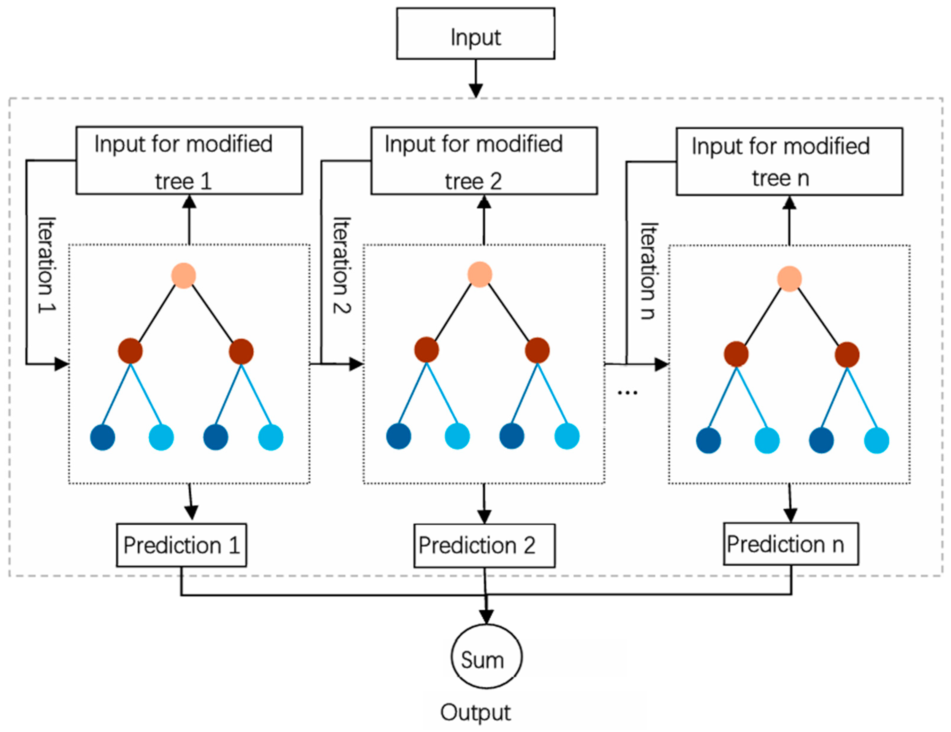
The integration of multiple classifiers through a Stacking ensemble learning methodology demonstrably enhances performance beyond that achieved by the selection of the best individual classifier [29]. This approach, when juxtaposed with current state-of-the-art techniques, consistently produces lower error rates and attains predictions of higher accuracy [30]. As a result of these findings, the Stacking ensemble learning strategy has achieved broad acclaim within the scientific community.

To improve the prediction accuracy of pollutant concentrations, we proposed a model based on Stacking ensemble learning. This model combines LSTM and XGBoost as base learners to capture different patterns in the PM2.5 data, and utilizes LightGBM as a meta-learner to integrate the outputs of the base learners, achieving optimal prediction performance. Empirical results demonstrate that the Stacking model can effectively capture the overall trends and patterns of actual PM2.5 concentrations, exhibiting particularly precise predictions in the tail region of the data. Although there are still some shortcomings in handling peak values and outliers, the model generally exhibits strong robustness and stable predictive ability for PM2.5 fluctuations. The Stacking model outperforms single models (such as CNN, LSTM, RF, XGB) in evaluation metrics such as mean squared error, root mean squared error, and mean absolute error, providing ample evidence that the ensemble learning framework effectively enhances generalization ability and prediction accuracy by integrating the strengths of multiple models. This model architecture reduces the potential biases of any single model and fully leverages the advantages of ensemble learning, offering an efficient solution for air quality prediction in Macau.

6. Conclusions

Through the analysis of meteorological and pollution data in Macau, we conducted data analysis, investigated the correlation with meteorological factors, and developed and evaluated prediction models. The main conclusions include the following:

• In Macau, PM2.5 and PM10 concentrations exhibit significant seasonal patterns, with higher concentrations in winter and lower concentrations in summer.
• Relative humidity, temperature, and sea-level pressure were identified as key meteorological factors influencing PM2.5 concentrations.
• Through hourly analysis, daytime and early morning were determined as peak periods for PM pollution in Macau.
• In Macau, PM is correlated with atmospheric stability but shows no significant correlation with boundary layer height.
• A PM2.5 concentration prediction model based on Stacking ensemble learning was proposed, employing LSTM and XGBoost as base learners and LightGBM as the meta-learner, significantly improving prediction accuracy.
• Experimental validation demonstrated that the constructed Stacking model can effectively capture the overall trends and patterns of PM2.5 concentrations, outperforming single models in evaluation metrics and reflecting the superiority of ensemble learning.

We systematically analyzed the PM pollution issue in Macau, ranging from the temporal characteristics of pollutants and the correlation with influencing factors, to the development of an innovative prediction model, yielding valuable research outcomes. Our work provides technological support for improving air quality in Macau and the broader region. Our findings not only enrich the research content in the field of air pollution in Macau but also provide new insights for air quality monitoring and control in other cities, possessing significant theoretical value and practical significance.

References

1. Kucbel, M.; Corsaro, A.; Švédová, B.; Raclavská, H.; Raclavský, K.; Juchelková, D. Temporal and seasonal variations of black carbon in a highly polluted European city: Apportionment of potential sources and the effect of meteorological conditions. J. Environ. Manag. 2017, 203, 1178–1189. [Google Scholar] [CrossRef] [PubMed]
2. Burnett, R.; Chen, H.; Szyszkowicz, M.; Fann, N.; Hubbell, B.; Pope, C.A., III; Apte, J.S.; Brauer, M.; Cohen, A.; Weichenthal, S.; et al. Global estimates of mortality associated with long-term exposure to outdoor fine particulate matter. Proc. Natl. Acad. Sci. USA 2018, 115, 9592–9597. [Google Scholar] [CrossRef]
3. Losacco, C.; Perillo, A. Particulate matter air pollution and respiratory impact on humans and animals. Environ. Sci. Pollut. Res. 2018, 25, 33901–33910. [Google Scholar] [CrossRef] [PubMed]
4. Švédová, B.; Kucbel, M.; Raclavská, H.; Růžičková, J.; Raclavský, K.; Sassmanová, V. Water-soluble ions in dust particles depending on meteorological conditions in urban environment. J. Environ. Manag. 2019, 237, 322–331. [Google Scholar] [CrossRef] [PubMed]
5. Švédová, B.; Raclavská, H.; Kucbel, M.; Růžičková, J.; Raclavský, K.; Koliba, M.; Juchelková, D. Concentration variability of water-soluble ions during the acceptable and exceeded pollution in an industrial region. Int. J. Environ. Res. Public Health 2020, 17, 3447. [Google Scholar] [CrossRef] [PubMed]
6. Zhang, Y.-L.; Cao, F. Fine particulate matter (PM2.5) in China at a city level. Sci. Rep. 2015, 5, 14884. [Google Scholar] [CrossRef] [PubMed]
7. Lei, T.M.; Ma, M.F. The Relationship between Roadside PM Concentration and Traffic Characterization: A Case Study in Macao. Sustainability 2023, 15, 10993. [Google Scholar] [CrossRef]
8. Liang, Y.-C.; Maimury, Y.; Chen, A.H.-L.; Juarez, J.R.C. Machine learning-based prediction of air quality. Appl. Sci. 2020, 10, 9151. [Google Scholar] [CrossRef]
9. Díaz-Robles, L.A.; Ortega, J.C.; Fu, J.S.; Reed, G.D.; Chow, J.C.; Watson, J.G.; Moncada-Herrera, J.A. A hybrid ARIMA and artificial neural networks model to forecast particulate matter in urban areas: The case of Temuco, Chile. Atmos. Environ. 2008, 42, 8331–8340. [Google Scholar] [CrossRef]
10. Pak, U.; Ma, J.; Ryu, U.; Ryom, K.; Juhyok, U.; Pak, K.; Pak, C. Deep learning-based PM2.5 prediction considering the spatiotemporal correlations: A case study of Beijing, China. Sci. Total Environ. 2020, 699, 133561. [Google Scholar] [CrossRef]
11. Chae, S.; Shin, J.; Kwon, S.; Lee, S.; Kang, S.; Lee, D. PM10 and PM2.5 real-time prediction models using an interpolated convolutional neural network. Sci. Rep. 2021, 11, 11952. [Google Scholar] [CrossRef] [PubMed]
12. Zhang, Y.; Yan, Q. A spatiotemporal model for PM2.5 prediction based on the K-Core idea and label distribution. Meteorol. Appl. 2023, 30, e2115. [Google Scholar] [CrossRef]
13. Mok, K.; Tam, S. Short-term prediction of SO2 concentration in Macau with artificial neural networks. Energy Build. 1998, 28, 279–286. [Google Scholar] [CrossRef]
14. Hoi, K.; Yuen, K.; Mok, K. Kalman filter based prediction system for wintertime PM10 concentrations in Macau. Glob. NEST J. 2008, 10, 140–150. [Google Scholar]
15. Vong, C.-M.; Ip, W.-F.; Wong, P.-k.; Yang, J.-y. Short-term prediction of air pollution in Macau using support vector machines. J. Control Sci. Eng. 2012, 2012, 518032. [Google Scholar] [CrossRef]
16. Fong, I.H.; Li, T.; Fong, S.; Wong, R.K.; Tallon-Ballesteros, A.J. Predicting concentration levels of air pollutants by transfer learning and recurrent neural network. Knowl.-Based Syst. 2020, 192, 105622. [Google Scholar] [CrossRef]
17. Lei, T.M.; Siu, S.W.; Monjardino, J.; Mendes, L.; Ferreira, F. Using machine learning methods to forecast air quality: A case study in Macao. Atmosphere 2022, 13, 1412. [Google Scholar] [CrossRef]
18. Lei, T.M.T.; Ng, S.C.W.; Siu, S.W.I. Application of ANN, XGBoost, and Other ML Methods to Forecast Air Quality in Macau. Sustainability 2023, 15, 5341. [Google Scholar] [CrossRef]
19. Yang, X.; Jiang, L.; Zhao, W.; Xiong, Q.; Zhao, W.; Yan, X. Comparison of ground-based PM2.5 and PM10 concentrations in China, India, and the US. Int. J. Environ. Res. Public Health 2018, 15, 1382. [Google Scholar] [CrossRef]
20. Hu, M.; Wang, Y.; Wang, S.; Jiao, M.; Huang, G.; Xia, B. Spatial-temporal heterogeneity of air pollution and its relationship with meteorological factors in the Pearl River Delta, China. Atmos. Environ. 2021, 254, 118415. [Google Scholar] [CrossRef]
21. Tritscher, T.; Raz, R.; Levi, Y.; Levy, I.; Broday, D.M. Emissions vs. turbulence and atmospheric stability: A study of their relative importance in determining air pollutant concentrations. Sci. Total Environ. 2020, 733, 139300. [Google Scholar]
22. Zhao, D.; Xin, J.; Gong, C.; Quan, J.; Liu, G.; Zhao, W.; Wang, Y.; Liu, Z.; Song, T. The formation mechanism of air pollution episodes in Beijing city: Insights into the measured feedback between aerosol radiative forcing and the atmospheric boundary layer stability. Sci. Total Environ. 2019, 692, 371–381. [Google Scholar] [CrossRef]
23. Amasyali, M.F.; Ersoy, O.K. Classifier ensembles with the extended space forest. IEEE Trans. Knowl. Data Eng. 2013, 26, 549–562. [Google Scholar] [CrossRef]
24. LeCun, Y.; Bottou, L.; Bengio, Y.; Haffner, P. Gradient-based learning applied to document recognition. Proc. IEEE 1998, 86, 2278–2324. [Google Scholar] [CrossRef]
25. Schmidhuber, J.; Hochreiter, S. Long short-term memory. Neural Comput 1997, 9, 1735–1780. [Google Scholar]
26. Breiman, L. Random forests. Mach. Learn. 2001, 45, 5–32. [Google Scholar] [CrossRef]
27. Chen, T.; Guestrin, C. Xgboost: A scalable tree boosting system. In Proceedings of the 22nd ACM SIGKDD International Conference on Knowledge Discovery and Data Mining, San Francisco, CA, USA, 13–17 August 2016. [Google Scholar]
28. Ke, G.; Meng, Q.; Finley, T.; Wang, T.; Chen, W.; Ma, W.; Ye, Q.; Liu, T.-Y. Lightgbm: A highly efficient gradient boosting decision tree. In Advances in Neural Information Processing Systems 30; Neural Information Processing Systems Foundation, Inc. (NeurIPS): La Jolla, CA, USA, 2017. [Google Scholar]
29. Džeroski, S.; Ženko, B. Is combining classifiers with stacking better than selecting the best one? Mach. Learn. 2004, 54, 255–273. [Google Scholar] [CrossRef]
30. Divina, F.; Gilson, A.; Goméz-Vela, F.; García Torres, M.; Torres, J.F. Stacking ensemble learning for short-term electricity consumption forecasting. Energies 2018, 11, 949. [Google Scholar] [CrossRef]
Figure 1. The daily average concentrations (in μg/m3 units) of PM10 (a) and PM2.5 (b) from 2015 to 2023 (solid line) and from 2020 to 2022 (bar chart).
Applsci 14 05062 g001
Figure 2. Concentration (in μg/m3 units) variations for PM10 (a) and PM2.5 (b) from 2020 to 2022 on a daily basis (solid line), and from 2015 to 2023 on a monthly (red bars chart) and seasonal (gray bars chart) basis.
Applsci 14 05062 g002
Figure 3. Hourly probability distribution (shading) and hourly average (white solid line) of PM10 (a) and PM2.5 (b) concentrations (in μg/m3 units) from 2020 to 2022.
Applsci 14 05062 g003
Figure 4. Heat map of the overall correlation between pollutants and meteorological factors. A double asterisk (**) indicates the p-value is less than 0.01.
Applsci 14 05062 g004
Figure 5. Same as Figure 4, but for spring (a), summer (b), autumn (c) and winter (d). An asterisk (*) indicates the p-value is less than 0.05, and a double asterisk (**) indicates the p-value is less than 0.01.
Applsci 14 05062 g005
Figure 6. CNN structure.
Applsci 14 05062 g006
Figure 7. LSTM structure.
Applsci 14 05062 g007
Figure 8. RF structure.
Applsci 14 05062 g008
Figure 9. XGBoost structure.
Applsci 14 05062 g009
Figure 10. LightGBM structure.
Applsci 14 05062 g010
Figure 11. The actual and predicted PM2.5 concentrations (in μg/m3 units) of CNN (a), LSTM (b), RF (c), XGBoost (d), and Stacking (e) models.
Applsci 14 05062 g011