Abstract
In this study, the satellite data of ASTER and Landsat 8 OLI were used for the discrimination of lithological units covering the Khyber range. Of the 24 tested band combinations, the most suitable include 632 and 468 of ASTER and 754 and 147 of OLI in the RGB sequence. The data were also tested with two conventional machine learning algorithms (MLAs), namely maximum likelihood classification (MLC) and support vector machine (SVM), for lithological mapping. Principal component analysis (PCA), minimum noise fraction (MNF), band ratios, and color composites in combination with available lithological maps and field data were utilized for training sample collection for the MLC and SVM models to classify the lithological units. The accuracy assessment of SVM and MLC was performed using a confusion matrix, which revealed a higher accuracy of 74.8419% and 72.1217% for ASTER and an accuracy of 58.4833% and 60.0257% for OLI, respectively. The results indicate that ASTER imagery is more suitable for lithological discrimination in the study area due to its high spectral resolution in the VNIR to SWIR range. The experiment revealed that the SVM classification offered the highest overall accuracy of nearly 75% and the kappa coefficient value of 0.7 on ASTER data. This demonstrates the effectiveness of SVM classification in exploring lithological mapping in dry to semi-arid regions.
1. Introduction
One of the significant components in geology is the mapping of the various units of rocks exposed on Earth’s surface, which is called lithological mapping. A lithological map by itself provides a great amount of enlightenment on rock characteristics and is very vital for economic geology. Lithological unit mapping can provide details on the spatial distribution of various rock units and their structural occurrences, which can be used to analyze and map potential mineralization zones [1,2,3,4,5,6,7]. Remote sensing (RS) has gained popularity as a cost-effective and effective tool for regional lithological mapping, particularly in arid and semi-arid environments [8,9,10,11]. For many years, optical imagery collected by airborne and spaceborne sensors has been used extensively in mineral and lithological exploration. Different rock types can display unique spectral absorption or reflection patterns in the pertinent electromagnetic spectrum, depending on their mineral compositions [12]. In the near-infrared (NIR), short-wave infrared (SWIR), and thermal infrared (TIR) spectral ranges, several minerals exhibit discriminative behavior [12,13,14]. Remote sensing sensors capture electromagnetic (EM) spectra of various wavelengths that are reflected or absorbed in order to identify materials based on their usual response as a result of varied chemical and physical attributes. Therefore, researchers use the RS data spectral bands to study and identify various lithologies using a variety of methodologies. Large-scale mapping may be performed affordably with multispectral satellite sensors like Landsat 8 and the Advanced Spaceborne Thermal Emission and Reflection Radiometer (ASTER). ASTER, launched in 1999 on the Terra platform, has three VNIR, six SWIR, and five TIR spectral bands with spatial resolutions of 15, 30, and 90 m, respectively [15]. On the other hand, Landsat 8 Operational Land Imager (OLI) and Thermal Infrared Sensor (TIRS) images consist of nine spectral bands with a spatial resolution of 30 m for Bands 1 to 7 and 9. Aerosol and coastal research benefit from the usage of the new band 1 (ultra-blue). The new band 9 is helpful in detecting cirrus clouds.
In the literature, multispectral Landsat, Sentinel 2, and ASTER images have been widely utilized for geological structure mapping, lithology discrimination, geohazard identification and mitigation, geomorphology and landform processes, and mineral exploration [14,16,17,18,19,20,21]. Digital image processing is the field of RS defined as the creation of modified images that contain more information to support the visual interpretation of features by manipulating remotely sensed data. Due to its higher spectral resolution in the SWIR and TIR region than other multispectral data, ASTER has a greater potential to perform semi-quantitative mineral mapping. This has allowed it to become the most popular form of imaging in geological research, particularly in hydrothermal alteration and lithological unit differentiation [20,22,23,24]. Even though the SWIR sensor of ASTER has not been active since 2008, about 4 million images with nearly worldwide land coverage have been recorded [25] with SWIR bands and are available for use. Principal component analysis (PCA), band ratios, MNF, and decorrelation stretching have all been widely utilized to map various lithologies, mostly using ASTER [2,6,7,9,24,25,26,27], Landsat 8 OLI [2,3,7], and Sentinel-2 [4,5,6] or their fused combination [3,6,7,9,24,25,26,27,28].
Machine learning algorithms can be grouped into four main categories: supervised, unsupervised, self-supervised, and reinforcement learning algorithms [29]. Supervised algorithms are utilized to forecast the outputs that fit the provided targets. Unsupervised techniques including clustering, PCA, and decorrelation stretching (DS) are used in the preprocessing stage before the ML algorithm to improve the accuracy of the data annotation [3,30]. In the literature, fused Sentinel-2 + ASTER data produced an SVM accuracy of 83.16% [31]; Sentinel-2 data produced MLC accuracy rates of 70% [32] and 76% [33]. So, various ML algorithms outperform one another for different lithological formations when using a variety of satellite data [34]. Due to their nonparametric methodology and capacity to identify complex decision boundaries, SVM, deep learning, and neural network-based algorithms are now the most popular [35]. Lithological unit classification from multispectral and hyperspectral data is often performed at the pixel level. This is achieved by applying analytical techniques that either use spectral parameters, such as the depths and symmetry of the absorption features, spectral slopes at particular wavelengths, and band ratios, or match a series of candidate spectra from a spectral library (in the field or laboratory) with the pixel spectra (in an image) [36]. USGS spectral library values of some common minerals found in lithological units of the study area are shown in Figure 1.
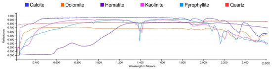
Figure 1.
The laboratory reflectance spectra of hematite, epidote, calcite, muscovite, illite, and kaolinite extracted from the USGS Spectral library [37].
This study investigated how remotely sensed data are able to assist in the discrimination of the lithological character of geological formations in the Khyber range, located near the Pakistan–Afghanistan border in KP, Pakistan (Figure 2). The attributes of different lithological units with respect to remotely sensed data have not been thoroughly studied in this region previously. The goal of this research is to determine the suitability of ASTER and Landsat 8 OLI data for discriminating the lithological character of the study area. The study also focuses on determining the best classifier between two common machine learning classifiers: maximum likelihood classification (MLC) and support vector machine (SVM), for lithological categorization of the study area.
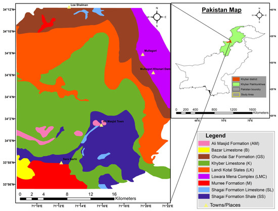
Figure 2.
Geological formation map of the study area, and the study area location [38].
2. Regional Geology and Tectonics
2.1. Study Area
The study area lies in the Khyber district between 71°9′0″ E and 71°22′0″ E longitude and between 33°56′0″ N and 34°12′0″ N latitude within the tribal belt of northwestern Pakistan. The Orakzai district lies to its south, the Kurram district to the southwest, and Peshawar to the east, whereas the Mohmand district lies to its north. It also borders the Nangarhar province of Afghanistan in the west.
2.2. Geological and Tectonic Framework
The Khyber range formed in the western portion of the lesser Himalayas. The fold and thrust belt of the Khyber range extends eastward up to the western margin of the Basham and Swat crystalline nappes after covering by alluvial deposits of the Peshawar basin [39]. Convergent tectonics transverse these ranges, which are highly deformed and are characterized by tight, asymmetrical, or isoclinal folds imbricated by several thrusts [40]. The Silurian and Devonian systems are reported from the axial belt of the Khyber and Nowshera–Swabi areas. The Punjal–Khairabad Fault System, which extends west from Gari Habibullah to the Khyber Pass region, is located to the north of the Khyber range [41]. The Khyber range constitutes a transition zone with an igneous–metamorphic complex in the north and sedimentary cover in the south [40]. To the north and south of the Khyber range are the Kohistan Island arc and Kalachitta–Margalla range bounded by MMT and MBT, respectively [42]. In the Late Triassic, postrift thermal subsidence led to marine sedimentation [43]. Late Paleozoic to early Paleozoic E-W-trending doleritic dikes were intruded into the Precambrian to Paleozoic rocks in the fold and thrust belt of the Khyber, Attock–Cherat, and Hazara ranges [41,44]. All the dikes and sills are found in the upper section of the Khyber limestone and are therefore younger than the Paleozoic section of the Khyber area.
2.3. Stratigraphic Setup of Khyber Area
The Khyber range exposes Paleozoic sedimentary successions such as the Cambrian Shagai formation, the Ordovician–Silurian Landi Kotal formation (LK), the Silurian–Devonian Ghundai Sar formation (GS), and the Devonian Khyber limestone (K). The Landikotal formation consists of an assemblage of slate, phyllite, and quartzite intruded by basic rocks. This Silurian–Devonian-age formation is structurally highly deformed with frequent repetition of strata. The dominant lithology in the Devonian Shagai formation is massively bedded micritic limestone. The Devonian Ali Masjid formation (AM) consists of sandstone at the lower portion and the presence of siltstone, volcanic ash, quartzite, and conglomeritic beds at the top. According to [45], Khyber limestone is dominantly composed of limestone with very little argillaceous and arenaceous partings. It has a medium- to fine-grained texture, a thick-bedded structure, and some recrystallization. The lower portion of this Carboniferous–Permian-age formation is more likely to include clays and layers of arenaceous limestone. Ghundai Sar formation is a belt of Silurian–Devonian coralline limestone exposed in the hills of Ghundai Sar, near Jamrud, Khyber district. The lithological composition of the Lowera Mena formation (LMC) is dominated by phyllite, phyllitic slates, and interbedded limestone with some quartzite. Quartz veins and granitic intrusion are also common. The Murree formation (M) is dominated by silty shale and sandstone occurring in association with Paleocene limestone. Bazar Limestone (B) is mostly limestone, but not much literature is available on its composition. All these formations are shown in the geological map of the study area in Figure 2.
2.4. Mineral Potential
The Khyber district possesses a wide variety of mineral resources. These deposits include marble, limestone, dolomite, soapstone, silica sand, barite, mica, and graphite. Semiprecious stones are also found at certain places within the district. Marble deposits are found in the Mullagbri, Sultan Khel, Ghundai Sar, and Loe Shalman areas of the Khyber district. Stratigraphically, the rocks containing marble extend continuously for about 14 km between Ghundai Sar in the south and Shahid Mena in the north. Limestone is abundantly available in the area and is the main source of building material for the area. The greater parts of almost all the high mountains of the area extending from Loe Shilman in the north to Aka Khel in the south are composed of limestone. Sizable reserves of dolomite are available in the Khyber district in the Shilman and Mullagori area (Figure 2). Some coal and fluorite presence has also been reported in the literature, and [46] also reported the presence of localized lead mineralization in carbonate rocks of Jamrud, Khyber, Pakistan.
3. Materials and Methods
3.1. Datasets
The two types of multispectral satellite imagery, ASTER and Landsat 8 OLI, utilized in this research were downloaded from the USGS EarthExplorer website (accessed on 12 January 2023) for free. In this investigation, the Khyber range, Pakistan, was covered by a single cloud-free ASTER Level 1 Precision Terrain Corrected Registered at Sensor Radiance (AST_L1T) picture. ASTER is an advanced multispectral sensor that was installed on the Terra spacecraft in December 1999. It has 14 spectral bands, including three VNIR bands with a 15 m spatial resolution, six SWIR bands with a 30 m spatial resolution, and five TIR bands with a 90 m spatial resolution (Figure 3). In order to provide stereoscopic capabilities, a further telescope is employed to look backward in the near-infrared spectral range (range 3B) [47]. The AST_L1T output is generated by the NASA Land Processes Distributed Active Archive Centre once the original AST_L1A image has undergone geometric, radiometric, and cross-talk corrections [48]. The level-1B ASTER data that were used in this study were collected on 15 May 2007.
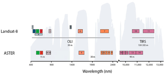
Figure 3.
Visual representation of the operational land imager (OLI) and ASTER sensors. Adapted from USGS Landsat Program [49]. ASTER: 1, green; 2, red; 3N/3B, NIR nadir-looking/NIR backward-looking; 4–9, SWIR; 10–14, TIR. Landsat-8: 1, coastal aerosol; 2, blue; 3, green; 4, red; 5, NIR; 6, SWIR 1; 7, SWIR 2; 8, panchromatic; 9, cirrus; 10, TIRS 1; 11, TIRS 2 [50].
Landsat 8 OLI (with OLI and TIRS sensors) of the Landsat series utilized in this study was launched by NASA on 11 February 2013. In comparison to Landsat 7 (ETM+), the OLI has two extra bands, including a new deep blue band for observing coastal areas and aerosols and an SWIR band for detecting cirrus (Figure 3). For lithological differentiation in this investigation, one OLI scene taken on 16 October 2022 was used. Even though these images were obtained in different seasons, the study area location is a perfectly exposed place for lithological classification with little to no plant cover. So, the effects of vegetation, clouds, or snow are not present in this study area.
3.2. Data Preprocessing
In order to remove the effects of water vapor and clouds and to convert the digital counts to surface reflectance, the ASTER and OLI bands were preprocessed using Environment for Visualising Images (ENVI). All the ASTER bands were radiometrically calibrated using the closest neighbor resampling approach and were resampled to 15 m resolution. The final nine-band ASTER picture was created by combining the three VNIR bands and six SWIR bands from the ASTER data, and a separate layer stack of TIR bands was also created. The first 7 OLI bands were also radiometrically calibrated using the closest neighbor resampling approach and were resampled to 30 m resolution. The Fast Line of Sight Atmospheric Analysis Spectral Hypercubes (FLAASH) atmospheric correction model incorporates the Moderate Resolution Transmittance (MODTRAN) radiation transfer code to remove the atmospheric attenuations to produce reflectance imagery, which is then used to calibrate the cross-talk-corrected nine bands of the ASTER image and seven bands of the OLI image to surface reflectance.
To obtain spatially and radiometrically corrected images for spectral data analysis and comparison, preprocessing processes were necessary. The ML task consisted of preprocessing, training, and testing the model. To transform the given data into a format that only provides relevant details about the problem, data preparation was necessary.
3.3. Minimum Noise Fraction (MNF)
Denoising the data from remote sensing is typically accomplished using the MNF [2]. A noisy data cube is transformed into output visuals with increasingly more noise. The outcome is a steady decline in the MNF output images’ image quality, as shown in Figure 4 for the ASTER MNF. The linear transformation process of the MNF involves two steps: (1) First, a noise covariance matrix is used to rescale and decorrelate noise in the data, a process known as noise whitening. Consequently, the noise has a unit variance, and no band-to-band correlations are present. (2) The noise-whitened data are often modified using the PCA approach.
Figure 4.
MNF of ASTER.
3.4. Principal Component Analysis (PCA)
During the preprocessing stage, the often-associated raw multidimensional dataset variables are transformed into a new set of uncorrelated variables, each of which is represented by a collection of principle components, using a statistical approach called principal component analysis (PCA). As a multivariate statistical data compression method, PCA reduces the dimensionality of the data by compressing redundant or correlated data into fewer bands [51]. A PCA produces independent, non-correlated output bands that are frequently easier to understand compared to the original data. As much of the data’s variability as possible can be explained by the first principal component, and as much of the remaining variability as possible can be explained by each subsequent component. Data variability is lowest for the first main component and increases for each subsequent component [52]. PCA enhances the spectral features of surface material by lowering the irradiance effects that predominate in all bands, removing duplicate data from several bands, and condensing information to a few significant selected bands. These bands are used as input for further examination by machine learning algorithms.
3.5. ASTER and OLI Band Combinations
Band combinations and false color composites (FCCs) are frequently employed for mineral and lithological mapping in order to highlight spectral characteristics between the target and background materials. This also reduces the impacts of changes in albedo and topographic slope [53,54,55,56].
3.6. Spectral Band Ratioing
By utilizing two spectral bands to compute a ratio image (division), band ratios highlight the spectral variations across mineral targets. This eliminates the topographic impact, which is roughly constant across all bands [57]. Bands are selected to draw attention to a specific material’s presence [58]. The process of band selection involves examining the target material’s spectral signature and selecting a wavelength band where the mineral appears bright due to high reflection and a band where it appears dark due to significant absorption. In order to obtain a higher ratio value (greater than 1.0) and make the target mineral look brighter in the ratio image, the more reflective band is employed as the numerator [59,60]. To distinguish the changed zones from the host rock, ratios were therefore built using the spectral characteristics of the lithologies. According to [61], adding images tends to accentuate information that is connected between bands and produces a compounded impact. Therefore, band ratios are helpful data reduction strategies that bring attention to the small spectrum differences hidden by the image’s brightness variations.
3.7. Machine Learning and Deep Learning-Based Techniques
Numerous machine learning techniques, including neural networks [62,63,64] and SVM, employ linear hyperplanes rather than other algorithms to distinguish between classes. For a variety of applications, such as mineral and lithological mapping [65], random forest (RF) [66,67] has been used extensively. If the classes are not linearly separable in the feature space, they are projected to a higher dimension to ensure linear separability [1,68,69,70]. To learn the boundaries of different classes in the feature space, each of these methods relies on pre-classified training data [35,71,72].
For lithological mapping, two popular machine learning algorithms—MLC and SVM—were utilized to determine which classifier would perform best for lithological classification. ASTER and Landsat 8 OLI multispectral data were evaluated for lithological classification in the Khyber range study area, resulting in a number of data combinations.
ASTER’s and OLI’s band configurations in the VNIR and SWIR range are anticipated to yield additional lithological unit diagnostic spectral characteristics. The SWIR and TIR bands are typically thought to be the most crucial for differentiating lithologies [12]. For example, limestone displays spectral alterations in the TIR range (10.25–11.65 m) and SWIR range (2.10–2.30 m) [73,74]. However, robust machine learning (ML) methods must be utilized to identify various rock types from limited data (without TIR bands). A streamlined sequence flow diagram of the aforementioned procedure is shown in Figure 5.

Figure 5.
Sequence flow diagram of the procedure used for lithological classification in the study.
3.7.1. Training and Testing Samples
More than 200 training samples were selected by carefully reviewing the geological formation map (Figure 2) and field data. The 14 bands of ASTER and 7 bands of OLI were used to classify lithological units. The study area is 641 km2 in size. The training dataset was meticulously chosen manually by taking into account the distributions and textural characteristics of the nine geological units shown in Figure 2. The MLC and SVM classifiers directly used the training datasets. Additionally, 110 randomly chosen ground truth locations from the research region were chosen as a testing dataset based on the geological map (Figure 2) and field data.
3.7.2. Supervised Classification Algorithms
In machine learning (ML) applications, the most frequently used supervised classification algorithms are SVM and MLC, which offer insightful information through cloud computing using geographical data. After machine learning models are trained using training data, their performance is assessed through cross-validation [51]. A classification function reduces the prediction error and often learns the complex input–output connection patterns to link the input data (features) with the output class or (target labels). The inputs are represented by n-vectors (X1, X2, …, Xn), while the results are given as finite k class labels (Y1, Y2, …, Yk). Training and testing sets are created from datasets. The lithological units in the study area were classified using two machine learning techniques, MLC and SVM. The used algorithms are briefly explained in the subsections that follow.
3.7.3. Maximum Likelihood Classifier
The maximum likelihood classification (MLC), initially suggested by German mathematician C.F. Gauss in 1821 for the normal distribution, is one of the most popular supervised classifiers in remote sensing [75,76,77]. This method, which is based on the assumption that the probability density function for each class is multivariate, assigns an unknown pixel to the class to which it has the highest possibility of belonging [75,78]. MLC is a widely used multivariate statistical classification technique that is included in a number of image processing software programs, including PCI, ERDAS, and ENVI. This classifier was applied to many datasets for lithological categorization in this work using ENVI 5.3 software, which was provided by Exelis Visual Information Solutions in the Boulder, CO, USA.
3.7.4. Support Vector Machine (SVM)
The mineral exploration industry commonly uses support vector machines (SVMs) to handle data from remote sensing [3,68,79,80]. SVM can offer nonlinear decision limits in high-dimensional variable space [81,82], which can be utilized to resolve a quadratic optimization problem [72]. SVM uses a hyperplane to categorize the provided dataset in an n-dimensional space as its classification method. The hyperplane that indicates the greatest gap between two classes is a logical option for the best hyperplane. It is possible to represent target detection using the SVM approach as a dichotomy.
Basic SVM theory states that several hyperplanes can separate different classes in a nonlinearly separable dataset with points from two classes. Only a portion of the “k” training samples—referred to as support vectors—are utilized to create the decision boundary, or the hyperplane that separates classes in the most efficient manner. The greatest decision boundary between the support vectors yields the best outcome across classes.
The lithological units were mapped using the ENVI SVM classifier on the basis of the training dataset. SVM received the chosen training data from the ML algorithm right away. The kernel type, cost parameter (C), and gamma coefficient are the three most important variables that have a major impact on SVM performance [1]. While the gamma parameter regulates the SVM model’s nonlinearity, the penalty parameter sets a limit on the amount of error that may be permitted in the training set. Trial and error were used to randomly modify the algorithm’s parameters in order to assess its performance. These cost (penalty) parameters were examined together with the gamma coefficient and other kernels.
According to a previous study [83], the SVM technique can use a variety of standard kernel functions, such as sigmoid, linear, polynomial, and radial basis functions. The accuracy of SVM training and classification depends on the choice of kernel functions. Since degree 1 polynomials are the simplest, they identify patterns more quickly than other kernels. For lithological mapping in this work, the SVM classifier built in ENVI was employed. The kernel type chosen was the radial basis function, the gamma in the kernel function was 0.091, and the penalty parameter was set to 100 [68].
3.7.5. Accuracy Measures
The efficacy of the MLC and SVM classifiers was assessed using the kappa coefficient, the producer accuracy (PA), and the user accuracy (UA), accuracies of the confusion matrix [84]. The ratio of accurate pixels to all of the pixels in the error matrix is known as the overall accuracy (OA), or pixels associated with class Y but mistakenly recognized as class Y. When pixels are categorized as class Y but are not connected to class Y, the UA provides commission errors as a sign of the algorithm’s reliability. The PA additionally includes the number of times an algorithm incorrectly labels a pixel as Y and omission mistakes for specific classes. Using random classification analyses to account for the possibility that agreements could emerge by accident, the kappa coefficient is a statistical indicator of how well a classified map agrees with reference data [85]. The kappa coefficient ranges from 0 to 1, with values closer to 0 indicating more categorization uncertainty and values closer to 1 indicating less. In order to verify the accuracy of the findings produced by these ML algorithms, fieldwork for ground truth observations was also conducted in the research region.
3.8. Lineament Mapping
A lineament is a region that undergoes deformation and fracturing, indicating a zone with increased secondary porosity that facilitates the flow of mineralized fluids. The PCI Geomatica Automatic Lineament Extraction algorithm (PCI-LINE) was utilized to map lineaments utilizing Landsat-8 data. Edge detection, thresholding, and curve extraction are the three steps that the PCI-LINE module typically uses to extract lineaments. ArcMap 10.5 was used to handle the extracted line segments, which included exporting the line segment shape file, modifying the line properties, and transforming complex lines into simple lines [86].
3.9. Field Data Validation
Fieldwork was also carried out at the study area to validate the lithological mapping results of remote sensing studies, and rock samples were also analyzed for petrographic studies to identify mineralogical compositions. Details of field and laboratory studies are discussed in Section 5.
4. Results
4.1. Minimum Noise Fraction (MNF) Transformation
After the MNF method was applied to the OLI and ASTER subset data, a substantial decline in eigenvalue magnitude vs. MNF band number occurred between 1 and 7 for OLI and between 1 and 9 for ASTER. In order to enhance the outcomes of the subsequent spectral processing, MNF components with eigenvalues less than 1 are frequently eliminated from the data as noise [87]. As a result, for further data processing, all nine bands of the ASTER data and the seven bands of the OLI data were kept. The greatest information is often carried by the first few MNF bands, whereas the noise level in later bands increases. It was clear from a visual examination of the MNF bands that a heterogeneous surface composition was possible in the research region.
4.2. Principal Component Analysis (PCA)
The results of the PCA are displayed in Figure 6 and Figure 7. To obtain the greatest visualization results, we further allocated these PC bands to RGB band combinations for color composite production as shown in Figure 6 and Figure 7. The ASTER RGBs include PC1, PC4, PC6 (Figure 6a) and PC3, PC5, PC7 (Figure 6b). The OLI RGBs include PC1, PC3, PC4 (Figure 7a) and PC2, PC4, PC7 (Figure 7b). These PC band RGB combinations of ASTER and OLI are shown to significantly discriminate the lithologies in the study area (Figure 6 and Figure 7).
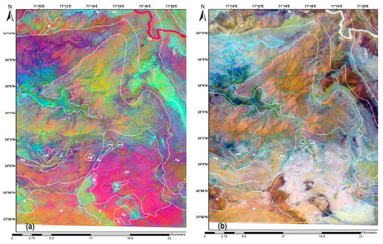
Figure 6.
(a) ASTER RGB of PC1, PC4, PC6. (b) ASTER RGB of PC3, PC5, PC7. The boundaries of geological formations (Figure 2) are marked in white color in these figures to show PCA classification in relation to the geological map.

Figure 7.
(a) Landsat OLI RGB of PC1, PC3, PC4. (b) Landsat OLI RGB of PC2, PC4, PC7. The boundaries of geological formations (Figure 2) are marked in white color in these figures to show PCA classification in relation to the geological map.
4.3. Color Composite
Based on the known spectral characteristics of the alteration minerals and rocks with respect to the chosen spectral bands, false color composites were created for OLI and ASTER using ENVI. To map the lithological units for this investigation, many different false color composites were created using different band combinations, but those providing better results than others on the basis of geological map and field data are shown in Figure 8 and Figure 9. Carbonate minerals, such as calcite and dolomite, can be identified using the SWIR bands of ASTER, and the CO3 group can be highlighted using ASTER TIR bands. Band 8 of the ASTER SWIR dataset records the CO3 absorption feature at a wavelength of 2.34 µm, which is the diagnostic absorption trough for carbonate-rich lithologies [88].

Figure 8.
(a) ASTER color composite (RGB:632). (b) ASTER color composite (RGB:468). The boundaries of geological formations (Figure 2) are marked in white color in these figures to show PCA classification in relation to the geological map.

Figure 9.
(a) OLI color composite (RGB:754). (b) OLI color composite (RGB:147). The boundaries of geological formations (Figure 2) are marked in white color in these figures to show PCA classification in relation to the geological map.
4.4. Band Ratios
In order to improve the spectral emissivity pattern of quartz, we used the quartz index (QI), a ratio proposed in [89] which is based on bands 10–13 of ASTER, and the result is shown in Figure 10. Quartz has a more pronounced spectral emissivity pattern with emissivities in the range 0.30–1.00 (Figure 1). Quartz has a lower spectral emissivity in bands 10 and 12, and the spectral emissivity patterns of quartz-bearing rocks also exhibit the Reststrahlen property.
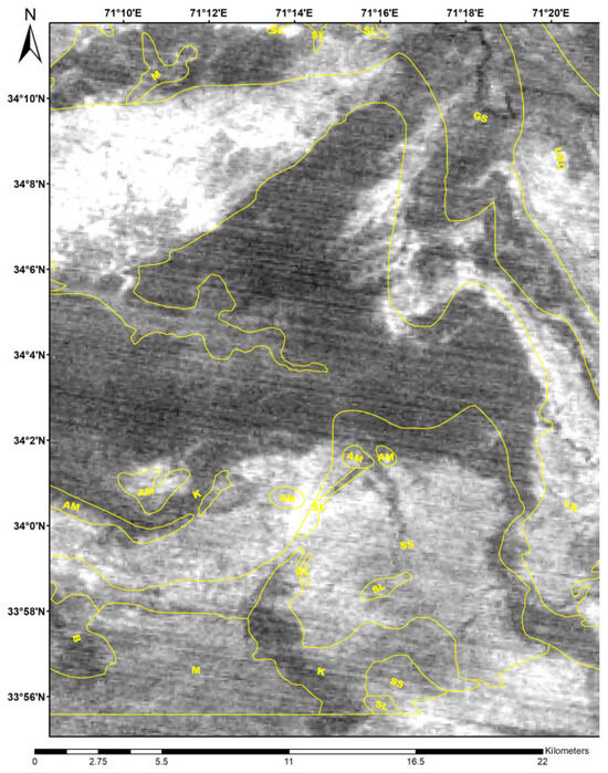
Figure 10.
Quartz index = (band 11/(band 10 + band 12))*(band 13/band 12). The bright pixels represent quartz dominance.
To discriminate carbonate minerals in the study area, we used ASTER L2 TIR ratio band 13/band 14 (Figure 11), as employed in [89] to successfully delineate carbonate minerals in Nevada. The emissivity feature of carbonate minerals is a result of CO3 vibrations in the TIR region at ASTER band 14. Because of the influence of temperature information, carbonate minerals’ spectral emissivity is weaker than quartz’s and may be difficult to identify in the ASTER L1B daytime TIR FCC image.
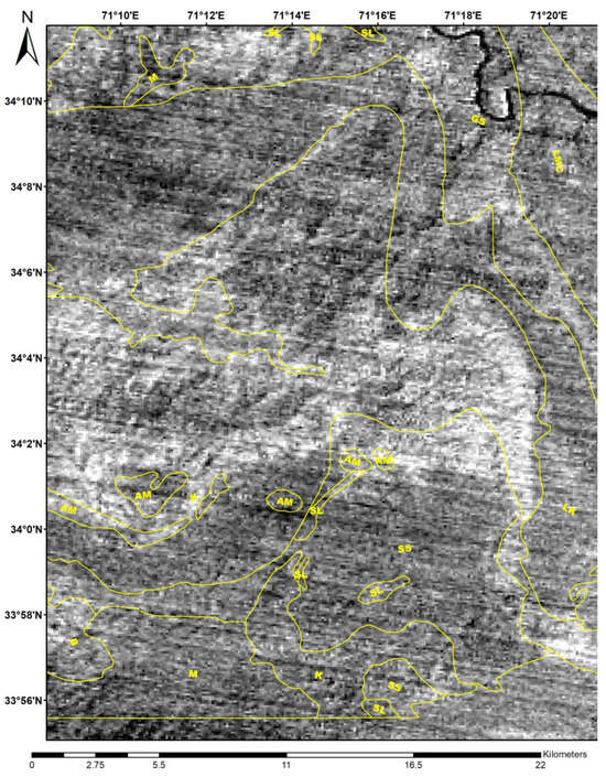
Figure 11.
Carbonate ratio = band 13/band 14. The bright pixels represent quartz dominance.
4.5. SVM and MLC Classification Results
To optimize the lithological classification of the study area using remote sensing data, we experimented with training SVM and MLC with different combinations of input data selected from ASTER and OLI images. ROIs covering different lithological units were selected using the field data, literature, and the preceding geological maps. The SVM and MLC image classification results are shown in Figure 12 and Figure 13, respectively. Following the algorithm classification results, the classification’s accuracy is evaluated by creating a confusion matrix and pixel-by-pixel comparing the output with the geological map and field data. Reviewing the confusion matrix of SVM reveals kappa values of 0.7 and 0.5036 and overall accuracy rates of 74.8419% and 58.4833% for ASTER and OLI, respectively. Reviewing the confusion matrix of MLC reveals kappa values of 0.6764 and 0.5398 and overall accuracy rates of 72.1217% and 60.0257% for ASTER and OLI, respectively.

Figure 12.
(a) ASTER SVM classification showing mapping results for different lithologies: Murree formation in dark greyish, Ghundai Sar formation in brownish color, Khyber limestone as mostly red, Shagai formation shale as dark green, river as yellow. (b) OLI SVM classification results showing different lithologies mapped: Murree formation in greenish color, Ghundai Sar formation in orchid purple, Khyber limestone as mostly sky-blue color, Shagai formation shale as navy-blue color, Bazar limestone as blue color, river as magenta color. The boundaries of geological formations (Figure 2) are marked in white color in these figures to show SVM classification in relation to the geological map.
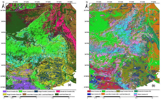
Figure 13.
(a) ASTER MLC classification results, showing different lithologies mapped; Murree formation in royal purple color, Ghundai Sar formation in pink color, Khyber limestone as mostly light green color. (b) OLI MLC classification results showing different lithologies mapped: Murree formation in bright pink color, Ghundai Sar formation in sea green color. The boundaries of geological formations (Figure 2) are marked in white color in these figures to show SVM classification in relation to the geological map.
With a polynomial kernel of degree 1 and a cost parameter of 0.02, SVM performs best at a gamma value of 1/6. Both algorithms received identical training samples, which were gathered after the data had been preprocessed. Good results were reported for both algorithms, with training and validation accuracy of over 70% for ASTER.
The PA and UA of MLC and SVM are shown in Table 1, Table 2, Table 3 and Table 4 and total ground truth pixels are shown in Table 5 for each lithological unit mapped, but unclassified and water values have been removed from these for a better understanding of lithological units. Using OLI, Ghundai Sar (GS) and Khyber limestone (K) had the highest UA for MLC classification, and the Ali Masjid formation (AM) had the highest UA for SVM classification. The UA of almost all formations was higher in SVM and MLC classifications using ASTER than those using OLI.

Table 1.
Confusion matrix of support vector machine (SVM) classification using ASTER.
Table 2.
Confusion matrix of maximum likelihood classification (MLC) using ASTER.
Table 3.
Confusion matrix of support vector machine (SVM) classification using OLI.
Table 4.
Confusion matrix of maximum likelihood classification (MLC) using OLI.
Table 5.
Total ground truth pixels of each class for MLC and SVM classifiers using OLI and ASTER.
5. Discussion
The remote sensing and ML methods discussed above were evaluated in this study for lithological classification of the well-exposed Khyber area having negligible plant cover. Irrational geological conclusions might result from human error coupled with inaccessibility to challenging terrain. Remote sensing can help explorers to identify specific regions of interest by geological mapping.
5.1. Principal Component Analysis (PCA)
In order to visualize the lithological variance, this study makes use of PCA- and MNF-transformed bands. The PCA approach yields results that compare favorably with existing geological maps and field data, indicating a very high level of accuracy. Since their eigenvalue and standard deviation statistics likewise show a contrastive broader range and cover maximum variability (Table 6 and Table 7), these composites effectively displayed maximal lithological discrimination.
Table 6.
Statistical details of eigenvectors of each ASTER band against the individual principal components.
Table 7.
Statistical details of eigenvectors of each OLI band against the individual principal components.
The combination of the first three main components (PCs 1, 2, and 3) was used in [90] to characterize the lithological variance of volcanic, meta-sedimentary, and sedimentary complexes. Using composites of one to five principal components from the ASTER dataset [91] mapped the host lithologies of igneous and sedimentary origin and delineated the various mineralized zones, such as the alteration zone, manganese, and serpentinite [91,92,93]. Similarly, for the Buka Daban mountain in northern Tibet, China, considerable sedimentary succession differentiation was accomplished thanks to different RGB combinations of MNF-transformed VNIR and SWIR bands from ASTER, Landsat-8, and Sentinel-2 satellite sensors [94]. In this study, we used PCs 1, 4, 6 and 3, 5, 7 of ASTER and PCs 1, 3, 4 and 2, 4, 7 of OLI as RGBs for lithological classification of the study area. Figure 6 and Figure 7 indicate that the combinations were very helpful for discriminating lithologies.
5.2. Color Composites
Numerous researchers have used various color composite techniques to identify different lithologies [95,96,97,98,99,100,101,102]. A review of the literature has shown that there is no strict rule dictating the use of any particular color composite combination for lithological mapping. The color composite combinations that effectively discriminated the lithologies in the study area included RGB:632, RGB:468 and RGB:754, RGB:147 of ASTER and OLI, respectively, as shown in Figure 8a,b and Figure 9a,b. The Murree formation (M), Shagai formation shale (SS), Ghundai Sar formation (GS), and Lowara Mena complex (LMC) have been very well mapped by these combinations. The contact between Ghundai Sar formation (GS), Lowara Mena complex (LMC), Landi Kotal slates (LK), Khyber limestone (K), and Murree formation (M) is clearly marked.
Fieldwork was carried out to collect samples for laboratory studies and to cross-check the relationship between remote sensing results and field observations, as shown in Figure 14. Overall good results were obtained using FCC in this study, highlighting the areas of changing lithological character that could be matched with field results (Figure 14). Using an RGB band combination makes it simple to identify lithological contacts and can greatly aid with the laborious lithological contact mapping in the field. To use this strategy, one must be aware of the targeted pixels’ highly reflecting peaks, which will make them stand out as bright pixels. For instance, the ASTER RGB:468 composite suggests that all of the constituent materials—clays, iron oxides, and calcites—are mapped onto the red band because of their strong reflecting feature in band 4. Additionally, calcite exhibits a reflecting feature in band 6, indicating that the combination of red and green in the band combination RGB:468 causes calcite to exist in yellow-hued tints. Because calcite lacks iron, it has no absorption at band 6 and has absorption at band 8, which is caused by CO3. The electromagnetic spectrum’s SWIR area contains all of the chosen bands. Clays, carbonates, and sulfate minerals exhibit characteristic absorption characteristics in this wavelength range, resulting in unique colors on the image representing the dominant lithological character. These bands were chosen mainly because it is important to draw attention to the spectral diagnostic characteristics of carbonate band 4, sericite/illite band 6, and ferruginous alteration (iron oxides) band 8. Because all hydroxyl-containing minerals have a high reflectance in band 4, this band was chosen to emphasize the majority of clay minerals as brilliant red. The clay absorption feature is in the center of band 6, and the carbonate feature is at the center of band 8. Band 8 highlights the following elements: tourmaline, carbonates, biotite, and epidote. Figure 8b displays the findings for the normalized RGB:468 band combination of ASTER.
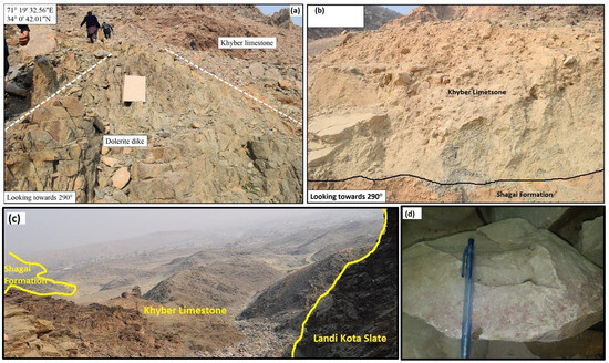
Figure 14.
(a) Oriented photograph showing dolerite intrusion in the Khyber limestone. These intrusions exist in the form of dikes and sills. (b) Field photograph showing contact between Khyber limestone and Shagai formation. (c) A distant view of the contacts between the outcrops of Landi Kotal slate, Khyber limestone, and Shagai formation in the study area. (d) Figure showing the sample from Ghundai Sar formation in the study area.
Since all hydroxyl-containing minerals are strongly reflective in band 4, standard RGB band combinations are unable to distinguish between them individually. This means that the detail to which typical color composites can be applied is limited. Nonetheless, standard RGB combinations remain helpful when attempting more intricate and sophisticated mapping approaches first and one has to obtain a rough idea of the geological makeup of the study area.
5.3. Band Ratios
Si–O stretching vibrations cause quartz to display a distinctive spectral emissivity pattern in the TIR range. Because of the spectral characteristics of quartz in ASTER bands 10, 11, and 12, the QI formula distinguishes the fine details in the QI image (Figure 10). The QI image produced by this formula using ASTER emissivity data identifies quartz-rich zones. The quartz index image is of higher quality when band 13 is used in the formula. QI image shows that most of the Landi Kotal slate (LK) and Shagai formation shale (SS) and part of the Lowara Mena complex (LMC) are dominated by the presence of quartz, and this can also be verified in the petrographic study results (Figure 15). The carbonate band ratio image (Figure 11) shows that most of the Khyber limestone (K) and part of the Ghundai Sar formation (GS) are dominated by the presence of carbonate, and this can also be verified in the petrographic study results (Figure 15).

Figure 15.
(a,b) Photomicrographs showing texture of phyllite and foliated basic rock from Landi Kotal slate. Weakly developed differential cleavage is defined by elongated fine-grained muscovite and elongated quartz grains. Oxide-filled veins crosscut the main fabric in the phyllite. (c) Photomicrograph of sample from Shagai formation showing calcite-filled fracture in a muddy matrix. (d) Sample collected from Khyber limestone, showing fractured spray to micritic limestone with recrystallized matrix and locally well-developed cross-hatched calcite crystals. The fracture in the rock is filled with opaque minerals that crosscut the main fabric of the recrystallized limestone.
5.4. Machine Learning Algorithms (MLAs)
The SVM and MLC approach classifies the studied lithological units in the study region with results very much matching the geological map, with some exceptions. In general, the ASTER sensor outperformed the OLI sensor, and the SVM outperformed the MLC for lithological classification of the study area. Additionally, the synthetic character of the borders between lithological units and the generalization used in the creation of geological maps both have an impact on the overall accuracy attained. The SVM well discriminated the Murree formation in both ASTER and OLI, represented in dark greyish and greenish color, respectively, in the resultant maps (Figure 12a,b). The SVM also well discriminated the Ghundai Sar formation in both ASTER and OLI, represented in dark greyish and greenish color, respectively, in the output SVM classification maps. The SVM classification for Khyber limestone using ASTER is shown as reddish, Shagai formation shale as dark green, and river as yellow color in Figure 12a. The SVM classification using OLI for the Ghundai Sar formation is shown in orchid purple, Khyber limestone in mostly sky-blue color, Shagai formation shale in navy-blue color, bazar limestone in blue color, and river in magenta color (Figure 12b). The MLC classification results for the Murree formation using ASTER are shown as royal purple color, Ghundai Sar formation as pink color, and Khyber limestone as mostly light green color in Figure 13a. The MLC classification using OLI for the Murree formation is shown in bright pink color and the Ghundai Sar formation in sea green color in Figure 13b. A total of nine lithological units were mapped in this research. A field visit was carried out to verify the classified lithologies on the ground, which indicated that the results of this study are mostly in accordance with the field features/lithologies (Figure 14). ML maps showed that the following lithostratigraphic units were detected in the field: Khyber limestone, Shagai formation, Landi Kotal slate, Lowara Mena complex. Khyber limestone covered the majority of the outcrops in the area that was mapped. The field validation and sample petrographic results also indicate a good correlation with the ML-produced lithological maps as shown in Figure 14 and Figure 15. The mineral compositions using petrographic studies of the samples from different lithologies (Landi Kotal slate, Shagai formation, Khyber limestone) of the study area are shown in Figure 15.
5.5. MLA Classification Accuracy
The classification accuracy of the lithological map produced from each classifier and dataset stated above was assessed using the following metrics: overall accuracy, producer accuracy, and kappa coefficient, which were derived from the confusion matrix. The overall accuracy may be calculated by dividing the total number of correctly identified pixels by the total number of test pixels. The likelihood that a classifier has accurately classified an image pixel is known as the producer’s accuracy, and the likelihood that a pixel has been properly categorized into its pre-specified class is known as the user’s accuracy. The kappa coefficient quantifies the level of agreement between the classified map and the reference data. The whole accuracy is not the same as the kappa coefficient, which assesses the consistency of the results and accounts for the entire contingency matrix [103]. The purpose of the evaluation was to compare the results of different methodologies and datasets in order to determine how successfully classification techniques may be utilized to map the lithology of the study region.
Even though the supervised technique MLC is counted among the best for many purposes, its utilization for lithology categorization in the Khyber area shows somewhat lower consistency as compared to SVM. Different rock units could differ in weathering susceptibilities due to differences in mineralogical composition, age, texture, and erosion rate [104]. This leads to a variety of topographic expressions in the field. For example, alluvium deposits frequently form flatlands, whereas igneous or metamorphic rocks, due to their low erosion, produce towering hills. The topographic behavior of lithologies could also be responsible for comparatively higher user and producer accuracy. For a better understanding of lithological discrimination, DEM data can be used for understanding the differences in analysis. The data from satellite-derived DEMs might be used to quantify the topographical manifestations of rock units (Figure 16).
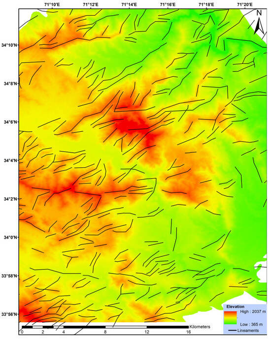
Figure 16.
Elevation profile of study area (from DEM) with extracted lineaments as black lines.
5.6. Discriminating Capability of ASTER and OLI
In order to discriminate alteration mineral associations, the Landsat OLI sensor has two SWIR bands [105,106,107,108,109,110]. Clay, sulfate, and carbonate types cannot be adequately distinguished by OLI SWIR bands [111]. In contrast, the ASTER instrument has five temperature bands and six SWIR bands, which can enhance the extraction of lithologic and mineral characteristics. The application of RS techniques for lithologic mapping and mineral prospecting is now the subject of many publications. The aforementioned classification study indicates that ASTER data are a more useful tool for lithologic mapping than OLI. The relative strength of OLI and ASTER data for lithological information extraction shows that the total accuracy of the mapping results obtained from the ASTER dataset in this investigation is higher than the values obtained from the OLI image (Table 1, Table 2, Table 3 and Table 4). This is because ASTER has a higher spatial resolution in the SWIR range than OLI, so the classification accuracy of lithological units obtained from the ASTER dataset is higher than that for the OLI dataset. Furthermore, because of the significant SWIR absorption properties of silicate minerals in ASTER bandpasses, ASTER is superior to OLI in the classification of different lithological units [112].
5.7. Comparison with Existing Maps
Using data from ASTER and OLI satellite imagery, the task of mapping different lithologies with mineralogical dissimilarities was successfully completed using remote sensing techniques and AI algorithms. Figure 17 is used to support the argument that the lithological detail and accuracy of the previously published geological map had improved. The current study’s integrated remote sensing-based approach effectively addresses these drawbacks of traditional geological mapping. Researchers [113] employed ASTER data along with field data to map the lithological variance within an accretionary complex. Geological mapping at 1:20,000 scale has been conducted using the same integrated remote sensing and field data methodology [114]. In the semi-arid northeastern Kohat plateau region of Pakatan, ref. [115] used PCA, band ratios, and false color composites as image processing and enhancement techniques to perform lithological differentiation. The lithology classification results in this study proved to be good with the exception of the Landi Kotal slates and Lowara Mena complex. The reason for this could be that the rock in this formation was not as exposed to the elements as other formations. Additionally, the mineralogical and chemical composition of the rock at the sub-pixel level, soil cover, vegetation coverage, atmospheric factors, and the image’s spatial and spectral resolution could all have an impact. SVM beats MLC in terms of accuracy for all forms, which suggests that it provides a more complete picture of the area. Also, ASTER shows more improved results than OLI, which could be due to ASTER data’s high resolution and strong computational efficiency. It is also necessary to look at how potential mineral mixing can affect the precision of lithologic classification and mapping using multispectral data. With this kind of study, it is possible to expand the data’s ability to discern equivalent lithologies outside the region of interest with high accuracy and minimum financial and computational costs.

Figure 17.
(a) Study area geological map with extracted lineaments in white color. (b) The lithological map generated from SVM classified using ASTER, with extracted lineaments as orange color lines.
As a result of the region’s substantial mineral potential, such automated mapping techniques would also help in the development of future exploration plans and technologies. Lineament mapping serves as a crucial roadmap for the exploration of mineral deposits and geological mapping [116,117]. Mineral exploration can benefit from the use of lineament markers like faults and fractures. Refinements in computer-aided spatial feature analysis should result in less human intervention in the process of geological mapping. Future research could use a sensor (improved hyperspectral) with high ground resolution (at least five meters) to map the areas more precisely. Drones can also have these sensors mounted in addition to satellites. Furthermore, the application of AI-based spatial estimation models [118] and surface maps to subsurface data (geophysical or geochemical) may be used to generate 3D geological models of potential mineralized zones. The strategies will allow the mining and mineral exploration industries to reach Industry 4.0 [119] by using blockchain [120] and IoT [121,122,123] technologies for safe data exchange.
The depth is one of the primary limitations of the remote sensing data as the various bands of electromagnetic radiation do not penetrate the surface of Earth. The remote sensing data are dependent only on the surficial features that reflect the electromagnetic energy of the sunlight. According to [124], the depth penetration of geological remote sensing is limited to a few centimeters in the TIR and only reaches the highest micrometers in the NIR (5–10 μm).
6. Conclusions
Remote sensing techniques and two popular supervised machine learning approaches (SVM and MLC) were utilized on multispectral data of ASTER and Landsat 8 to compare their efficiency in differentiating lithological units in the Khyber region. The remote sensing methods used in the study included principal component analysis (PCA), minimum noise fraction (MNF), band ratios, and color composites. Training samples for MLA were gathered on the basis of previously published geological maps and field data. The PCA and false color composites of ASTER were better than those of OLI for lithological discrimination of the study area. The lineament analysis of the research region showed that major and minor structures could be easily found in wide expanses of land and that this is, thus, a valuable technique for quickly obtaining an overview of the structural features of the area. The results show that the geological formations are mapped with >70% OA with the SVM approach using ASTER. The calculated accuracy assessment of SVM and MLC using a confusion matrix revealed a higher accuracy of 74.8419% and 72.1217% for ASTER and an accuracy of 58.4833% and 60.0257% for OLI, respectively. Overall, the results indicate that ASTER imagery has better potential for lithological discrimination in the study area and that the optimal approach in this case is SVM. A more detailed map of nine geological formations discriminating various lithological units was produced using ASTER and OLI satellite RS data. The study demonstrated that lithological mapping in any dry to semi-arid region could effectively be performed at a lower computing cost using such techniques on multispectral data.
From the comparisons and discussion, the following conclusions are reached:
- (1)
- ASTER has better results than OLI for using remote sensing and MLC and SVM machine learning techniques for the lithological discrimination of the Khyber range.
- (2)
- In semi-arid and dry regions like the Khyber range, SVM outperforms MLC in lithological classification.
Author Contributions
Conceptualization: S.A. and H.L.; methodology: S.A., H.L. and A.A.; software: S.A. and H.L.; validation, S.A.; formal analysis: S.A. and H.L.; investigation: S.A. and A.A.; data processing: S.A., H.L. and J.I.H.; writing—original draft preparation: S.A.; writing—review and editing: H.L., A.A. and J.I.H. All authors have read and agreed to the published version of the manuscript.
Funding
This study was supported by the National Natural Science Foundation of China (No. 92162103), the Natural Science Foundation of Hunan Province (No. 2022JJ30699, No. 2023JJ10064), and the Science and Technology Innovation Program of Hunan Province (No. 2021RC4055, No. 2022RC1182).
Institutional Review Board Statement
Not applicable.
Informed Consent Statement
Not applicable.
Data Availability Statement
The original contributions presented in the study are included in the article, further inquiries can be directed to the corresponding author.
Conflicts of Interest
The authors declare no conflicts of interest.
References
- Bachri, I.; Hakdaoui, M.; Raji, M.; Teodoro, A.C.; Benbouziane, A.; Cl, A. Machine Learning Algorithms for Automatic Lithological Mapping Using Remote Sensing Data: A Case Study from Souk Arbaa Sahel, Sidi Ifni Inlier, Western Anti-Atlas, Morocco. ISPRS Int. J. Geo-Inf. 2019, 8, 248. [Google Scholar] [CrossRef]
- Hamimi, Z.; Hagag, W.; Kamh, S.; El-Araby, A.M.A. Application of remote-sensing techniques in geological and structural mapping of Atalla Shear Zone and Environs, Central Eastern Desert, Egypt. Arab. J. Geosci. 2020, 13, 414. [Google Scholar] [CrossRef]
- Khan, M.F.A.; Muhammad, K.; Bashir, S.; Ud Din, S.; Hanif, M. Mapping Allochemical Limestone Formations in Hazara, Pakistan Using Google Cloud Architecture: Application of Machine-Learning Algorithms on Multispectral Data. ISPRS Int. J. Geo-Inf. 2021, 10, 58. [Google Scholar] [CrossRef]
- Köhler, M.; Hanelli, D.; Schaefer, S.; Barth, A.; Knobloch, A.; Hielscher, P.; Cardoso-Fernandes, J.; Lima, A.; Teodoro, A.C. Lithium potential mapping using artificial neural networks: A case study from central portugal. Minerals 2021, 11, 1046. [Google Scholar] [CrossRef]
- Merembayev, T.; Kurmangaliyev, D.; Bekbauov, B.; Amanbek, Y. A Comparison of Machine Learning Algorithms in Predicting Lithofacies: Case Studies from Norway and Kazakhstan. Energies 2021, 14, 1896. [Google Scholar] [CrossRef]
- Öztan, N.S.; Süzen, M.L. Mapping evaporate minerals by ASTER. Int. J. Remote Sens. 2011, 32, 1651–1673. [Google Scholar] [CrossRef]
- Sekandari, M.; Aminpour, S.M.; Masoumi, I.; Pour, A.B.; Muslim, A.M.; Rahmani, O.; Hashim, M.; Zoheir, B.; Pradhan, B.; Misra, A. Application of Landsat-8, Sentinel-2, ASTER and WorldView-3 Spectral Imagery for Exploration of Carbonate-Hosted Pb-Zn Deposits in the Central Iranian Terrane (CIT). Remote Sens. 2020, 12, 1239. [Google Scholar] [CrossRef]
- Zhang, X.; Li, P. Lithological mapping from hyperspectral data by improved use of spectral angle mapper. Int. J. Appl. Earth Obs. Geoinf. 2014, 31, 95–109. [Google Scholar] [CrossRef]
- Masoumi, F.; Eslamkish, T.; Honarmand, M.; Abkar, A.A. A comparative study of Landsat-7 and Landsat-8 data using image processing methods for hydrothermal alteration mapping. Resour. Geol. 2017, 67, 72–88. [Google Scholar] [CrossRef]
- Gad, S.; Kusky, T. Lithological mapping in the eastern desert of Egypt, the barramiya area, using Landsat Thematic Mapper (TM). J. Afr. Earth Sci. 2006, 44, 196–202. [Google Scholar] [CrossRef]
- Gad, S.; Kusky, T. ASTER spectral ratioing for lithological mapping in the Arabian–Nubian shield, the Neoproterozoic wadi kid area, Sinai, Egypt. Gondwana Res. 2007, 11, 326–335. [Google Scholar] [CrossRef]
- Gupta, R.P. Spectra of Minerals and Rocks. In Remote Sensing Geology; Springer: Berlin/Heidelberg, Germany, 2003; pp. 33–52. ISBN 978-3-662-05283-9. [Google Scholar]
- Van der Meer, F.D.; van der Werff, H.M.A.; van Ruitenbeek, F.J.A. Potential of ESA’s Sentinel-2 for geological applications. Remote Sens. Environ. 2014, 148, 124–133. [Google Scholar] [CrossRef]
- Van der Meer, F.D.; van der Werff, H.M.A.; van Ruitenbeek, F.J.A.; Hecker, C.A.; Bakker, W.H.; Noomen, M.F.; van der Meijde, M.; Carranza, E.J.M.; de Smeth, J.B.; Woldai, T.; et al. Multi- and hyperspectral geologic remote sensing: A review. Int. J. Appl. Earth Obs. Geoinf. 2012, 14, 112–128. [Google Scholar] [CrossRef]
- Yamaguchi, Y.; Kahle, A.B.; Tsu, H.; Kawakami, T.; Pniel, M. Overview of advanced spaceborne thermal emission and reflection radiometer (ASTER). IEEE Trans. Geosci. Remote Sens. 1998, 36, 1062–1071. [Google Scholar] [CrossRef]
- Mshiu, E.E. Landsat remote sensing data as an alternative approach for geological mapping in Tanzania: A case study in the Rungwe volcanic province, South-Western Tanzania. Tanz. J. Sci. 2011, 37, 26–36. [Google Scholar]
- Hewson, R.D.; Cudahy, T.J.; Mizuhiko, S.; Ueda, K.; Mauger, A.J. Seamless geological map generation using ASTER in the Broken Hill-Curnamona province of Australia. Remote Sens. Environ. 2005, 99, 159–172. [Google Scholar] [CrossRef]
- Graettinger, A.H.; Ellis, M.K.; Skilling, I.P.; Reath, K.; Ramsey, M.S.; Lee, R.J.; Hughes, C.G.; McGarvie, D.W. Remote sensing and geologic mapping of glaciovolcanic deposits in the region surrounding Askja (Dyngjufjöll) volcano, Iceland. Int. J. Remote Sens. 2013, 34, 7178–7198. [Google Scholar] [CrossRef]
- Asl, R.A.; Afzal, P.; Adib, A.; Yasrebi, A.B. Application of multifractal modeling for the identification of alteration zones and major faults based on ETM+ multispectral data. Arab. J. Geosci. 2015, 8, 2997–3006. [Google Scholar] [CrossRef]
- Pournamdari, M.; Hashim, M.; Pour, A.B. Application of ASTER and Landsat TM data for geological mapping of Esfandagheh ophiolite complex, southern Iran. Resour. Geol. 2014, 64, 233–246. [Google Scholar] [CrossRef]
- Masoumi, F.; Eslamkish, T.; Abkar, A.A.; Honarmand, M.; Harris, J.R. Integration of spectral, thermal, and textural features of ASTER data using random forests classification for lithological mapping. J. Afr. Earth Sci. 2017, 129, 445–457. [Google Scholar] [CrossRef]
- Crosta, A.; De Souza Filho, C.; Azevedo, F.; Brodie, C. Targeting key alteration minerals in epithermal deposits in Patagonia, Argentina, using ASTER imagery and principal component analysis. Int. J. Remote Sens. 2003, 24, 4233–4240. [Google Scholar] [CrossRef]
- Rowan, L.C.; Mars, J.C.; Simpson, C.J. Lithologic mapping of the Mordor, NT, Australia ultramafic complex by using the Advanced Spaceborne Thermal Emission and Reflection Radiometer (ASTER). Remote Sens. Environ. 2005, 99, 105–126. [Google Scholar] [CrossRef]
- Tangestani, M.H.; Jaffari, L.; Vincent, R.K.; Sridhar, B.M. Spectral characterization and ASTER-based lithological mapping of an ophiolite complex: A case study from Neyriz ophiolite, SW Iran. Remote Sens. Environ. 2011, 115, 2243–2254. [Google Scholar] [CrossRef]
- Tangestani, M.H.; Shayeganpour, S. Mapping a lithologically complex terrain using Sentinel-2A data: A case study of Suriyan area, southwestern Iran. Int. J. Remote Sens. 2020, 41, 3558–3574. [Google Scholar] [CrossRef]
- El Atillah, A.; El Morjani, Z.E.A.; Souhassou, M. Use of the Sentinel-2A Multispectral Image for Litho-Structural and Alteration Mapping in Al Glo’a Map Sheet (1/50,000) (Bou Azzer-El Graara Inlier, Central Anti-Atlas, Morocco). Artif. Satell. 2019, 54, 73–96. [Google Scholar] [CrossRef]
- Tripathi, M.K. Lithological Mapping using Digital Image Processing Techniques on Landsat 8 OLI Remote Sensing Data in Jahajpur, Bhilwara, Rajasthan. In Proceedings of the 2nd International Conference on Intelligent Communication and Computational Techniques (ICCT), Jaipur, India, 28–29 September 2019; pp. 43–48. [Google Scholar]
- Salehi, S.; Mielke, C.; Brogaard Pedersen, C.; Dalsenni Olsen, S. Comparison of ASTER and sentinel-2 spaceborne datasets for geological mapping: A case study from North-East Greenland. Geol. Surv. Denmark Greenl. Bull. 2019, 43, e2019430205. [Google Scholar] [CrossRef]
- Chollet, F. Deep Learning with Python, 1st ed.; Manning Publications Co.: Shelter Island, NY, USA, 2017; ISBN 1617294438. [Google Scholar]
- Othman, A.A.; Gloaguen, R. Integration of spectral, spatial and morphometric data into lithological mapping: A comparison of different Machine Learning Algorithms in the Kurdistan Region, NE Iraq. J. Asian Earth Sci. 2017, 146, 90–102. [Google Scholar] [CrossRef]
- Kabolizadeh, M.; Rangzan, K.; Mousavi, S.S.; Azhdari, E. Applying optimum fusion method to improve lithological mapping of sedimentary rocks using sentinel-2 and ASTER satellite images. Earth Sci. Inform. 2022, 15, 1765–1778. [Google Scholar] [CrossRef]
- Janati, M.H.; Soulaimani, A.; Admou, H.; Youbi, N.; Hafid, A.; Hefferan, K.P. Application of ASTER remote sensing data to geological mapping of basement domains in arid regions: A case study from the Central Anti-Atlas, Iguerda inlier, Morocco. Arab. J. Geosci. 2013, 7, 2407–2422. [Google Scholar] [CrossRef]
- Fal, S.; Maanan, M.; Baidder, L.; Rhinane, H. The contribution of Sentinel-2 satellite images for geological mapping in the south of Tafilalet basin (Eastern Anti-Atlas, Morocco). In Proceedings of the 5th International Conference on Geoinformation Science—GeoAdvances, Casablanca, Morocco, 10–11 October 2018; The International Archives of the Photogrammetry, Remote Sensing and Spatial Information Sciences: Casablanca, Morrocco, 2019; Volume XLII-4/W12, pp. 75–82. [Google Scholar]
- Cheng, G.; Zhang, H.; Li, H.; Deng, X.; Elatikpo, S.M.; Li, J.; Hu, Z.; Li, G. Quantitative inversion of REEs in ion-adsorbed rare earth ores from the Liutang area (South China), based on measured hyperspectral data. J. Earth Sci. 2023, 34, 1068–1082. [Google Scholar] [CrossRef]
- Li, S.; Song, W.; Fang, L.; Chen, Y.; Ghamisi, P.; Benediktsson, J.A. Deep Learning for Hyperspectral Image Classification: An Overview. IEEE Trans. Geosci. Remote Sens. 2019, 57, 6690–6709. [Google Scholar] [CrossRef]
- Yokoya, N.; Chan, J.; Segl, K. Potential of resolution-enhanced hyperspectral data for mineral mapping using simulated EnMAP and Sentinel-2 images. Remote Sens. 2016, 8, 172. [Google Scholar] [CrossRef]
- USGS Spectral Characteristic Viewer. Available online: https://landsat.usgs.gov/spectral-characteristics-viewer (accessed on 20 February 2024).
- Shah, M.M.; Afridi, S.; Khan, E.U.; Rahim, H.U.; Mustafa, M.R. Diagenetic modifications and reservoir heterogeneity associated with magmatic intrusions in the Devonian Khyber Limestone, Peshawar Basin, NW Pakistan. Geofluids 2021, 2021, 8816465. [Google Scholar] [CrossRef]
- Treloar, P.J.; Broughten, R.D.; Coward, M.P.; Williams, M.P.; Windley, B.F. Deformation, Metamorphism and Imbrication of the Indian Plate South of MMT, North Pakistan. J. Metamorph. Geol. 1989, 7, 111–127. [Google Scholar] [CrossRef]
- Kazmi, A.H.; Jan, M.Q. Geology and Tectonics of Pakistan; Graphic Publishers: Karachi, Pakistan, 1997. [Google Scholar]
- Tahirkheli, R.K.; Mattauer, M.; Proust, F.; Tapponnier, P. The India-Eurasia suture zone in northern Pakistan: Synthesis and interpretation of recent data at plate scale. In Geodynamics of Pakistan; Farah, A., Jong, K.A., Eds.; Geological Survey of Pakistan: Quetta, Pakistan, 1979; pp. 125–130. [Google Scholar]
- DiPietro, J.A.; Pogue, K.R. Tectonostratigraphic Subdivisions of the Himalaya: A View from the West. Tectonics 2004, 23, TC5001. [Google Scholar] [CrossRef]
- Zhu, D.; Meng, Q.; Jin, Z.; Liu, Q.; Hu, W. Formation mechanism of deep Cambrian dolomite reservoirs in the Tarim basin, northwestern China. Mar. Pet. Geol. 2015, 59, 232–244. [Google Scholar] [CrossRef]
- Calkin, J.A.; Offield, T.W.; Abdullah, S.K.; Ali, S.T. Geology of the Southern Himalaya in Hazara, Pakistan, and Adjacent Areas; U.S. Geological Survey Professional Paper 716-C; United States Government Printing Office: Washington, DC, USA, 1975. [Google Scholar]
- Shah, S.M.I.; Siddiqui, R.A.; Talent, J.A. Geology of the Eastern Khyber Agency, North Western Frontier Province, Pakistan; Geological Survey of Pakistan: Quetta, Pakistan, 1980; Volume 44. [Google Scholar]
- Ali, A.; Ali, S.; Akbar, S.; Azad, A.; Danish, A.; Ahmad, R.; Ali, L. Lead Mineralization in Carbonate Rocks Jamrud, District Khyber, Pakistan. In Proceedings of the International Conference on Mediterranean Geosciences Union, Istanbul, Turkey, 25–28 November 2021; Springer Nature: Cham, Switzerland, 2021; pp. 117–122. [Google Scholar]
- Fujisada, H.; Iwasaki, A.; Hara, S. In ASTER stereo system performance. Proc. SPIE 2001, 4540, 39–49. [Google Scholar]
- Duda, K.; Daucsavage, J.; Siemonsma, D.; Brooks, B.; Oleson, R.; Meyer, D.; Doescher, C. Advanced Spaceborne Thermal Emission and Reflection Radiometer (ASTER) Level 1 Precision Terrain Corrected Registered At-Sensor Radiance Product (AST_L1T): AST_L1T Product User’s Guide, Version 1.1; USGS: Reston, VA, USA, 2020. [Google Scholar]
- United States Geological Survey (USGS). Landsat 8 Band Designations. Available online: https://www.usgs.gov/media/images/landsat-8-band-designations (accessed on 16 January 2020).
- USGS Landsat Program. Comparison of #Landsat 7, 8, #Sentinel 2, #ASTER & #MODIS Bands. View Band Designations for All #Landsat Sensors. Available online: https://twitter.com/usgslandsat/status/837696716417687553 (accessed on 22 December 2017).
- Crosta, A.P.; Rabelo, A. Assessing Landsat TM for hydrothermal alteration mapping in central-western Brazil. In Proceedings of the 9th Thematic Conference on Geologic Remote Sensing, Pasadena, CA, USA, 8–11 February 1993; Environmental Research Institute of Michigan: Pasadena, CA, USA, 1993; pp. 1053–1061. [Google Scholar]
- Hastie, T.; Tibshirani, R.; Friedman, J. The Elements of Statistical Learning: Data Mining, Inference, and Prediction, 2nd ed.; Springer Series in Statistics; Springer: New York, NY, USA, 2009; ISBN 9780387848587. [Google Scholar]
- Crowley, J.K.; Brickey, D.W.; Rowan, L.C. Airborne imaging spectrometer data of the Ruby Mountains, Montana: Mineral discrimination using relative absorption band-depth images. Remote Sens. Environ. 1989, 29, 121–134. [Google Scholar] [CrossRef]
- Sabins, F.F. Remote sensing for mineral exploration. Ore Geol. Rev. 1999, 14, 157–183. [Google Scholar] [CrossRef]
- Son, Y.S.; Kim, K.E.; Yoon, W.J.; Cho, S.J. Regional mineral mapping of island arc terranes in southeastern Mongolia using multispectral remote sensing data. Ore Geol. Rev. 2019, 113, 103106. [Google Scholar] [CrossRef]
- Son, Y.S.; You, B.W.; Bang, E.S.; Cho, S.J.; Kim, K.E.; Baik, H.; Nam, H.T. Mapping alteration mineralogy in eastern Tsogttsetsii, Mongolia, based on the WorldView-3 and field shortwave-infrared spectroscopy analyses. Remote Sens. 2021, 13, 914. [Google Scholar] [CrossRef]
- Shibata, Y. Application of ASTER Data to Mineral Exploration for Cyprus-Type Massive Sulphide Deposits of Oman Ophiolite. In ASTER Science Project Report; NASA: Washington, DC, USA, 2002. [Google Scholar]
- Smith, R.B. Hyperspectral Imaging. Getting Started with TNT Mips Software; Microimages PLC: Lincoln, NE, USA, 2001. [Google Scholar]
- Ninomiya, Y.; Fu, B.; Cudahy, T.J. Detecting lithology with Advanced Spaceborne Thermal Emission and Reflection Radiometer (ASTER) multispectral thermal infrared “radiance-at-sensor” data. Remote Sens. Environ. 2002, 84, 127–139. [Google Scholar] [CrossRef]
- Rowan, L.C.; Kahle, A.B. Evaluation of 0.46 to 2.36 µm Multispectral Scanner images of the East Tintic Mining District, Utah, for mapping hydrothermally altered rocks. Econ. Geol. J. 1982, 77, 441–452. [Google Scholar] [CrossRef]
- Mather, P.M. Computer Processing of Remotely Sensed Images. An Introduction; John Wiley & Sons, Ltd.: Hoboken, NJ, USA, 2001. [Google Scholar]
- Meng, Z.; Li, L.; Jiao, L.; Feng, Z.; Tang, X.; Liang, M. Fully Dense Multiscale Fusion Network for Hyperspectral Image Classification. Remote Sens. 2019, 11, 2718. [Google Scholar] [CrossRef]
- Tran, D.; Bourdev, L.; Fergus, R.; Torresani, L.; Paluri, M. Learning spatiotemporal features with 3d convolutional networks. In Proceedings of the IEEE International Conference on Computer Vision, Santiago, Chile, 13–16 December 2015; pp. 4489–4497. [Google Scholar]
- Zhou, B.; Lapedriza, A.; Xiao, J.; Torralba, A.; Oliva, A. Learning deep features for scene recognition using places database. In Advances in Neural Information Processing Systems 27 (NIPS 2014), Proceedings of the Annual Conference on Neural Information Processing Systems 2014, Montreal, QC, Canada, 8–13 December 2014; MIT Press: Cambridge, MA, USA, 2014; pp. 487–495. [Google Scholar]
- Chen, Y.; Wu, W.; Zhao, Q. A Bat-Optimized One-Class Support Vector Machine for Mineral Prospectivity Mapping. Minerals 2019, 9, 317. [Google Scholar] [CrossRef]
- Gislason, P.O.; Benediktsson, J.A.; Sveinsson, J.R. Random forests for land cover classification. Pattern Recognit. Lett. 2006, 27, 294–300. [Google Scholar] [CrossRef]
- Rodriguez-Galiano, V.F.; Ghimire, B.; Rogan, J.; Chica-Olmo, M.; Rigol-Sanchez, J.P. An assessment of the effectiveness of a random forest classifier for land-cover classification. ISPRS J. Photogramm. Remote Sens. 2012, 67, 93–104. [Google Scholar] [CrossRef]
- Othman, A.; Gloaguen, R. Improving lithological mapping by SVM classification of spectral and morphological features: The discovery of a new chromite body in the Mawat ophiolite complex (Kurdistan, NE Iraq). Remote Sens. 2014, 6, 6867–6896. [Google Scholar] [CrossRef]
- Jaakkola, T.; Haussler, D. Exploiting generative models in discriminative classifiers. In Advances in Neural Information Processing Systems 11 (NIPS 1998), Proceedings of the Annual Conference on Neural Information Processing Systems 1998, Denver, CO, USA, 1–3 December 1998; MIT Press: Cambridge, MA, USA, 1998; pp. 487–493. [Google Scholar]
- Melgani, F.; Bruzzone, L. Classification of hyperspectral remote sensing images with support vector machines. IEEE Trans. Geosci. Remote Sens. 2004, 42, 1778–1790. [Google Scholar] [CrossRef]
- Li, N.; Huang, X.; Zhao, H.; Qiu, X.; Deng, K.; Jia, G.; Gong, X. A Combined Quantitative Evaluation Model for the Capability of Hyperspectral Imagery for Mineral Mapping. Sensors 2019, 19, 328. [Google Scholar] [CrossRef]
- Clark, R.N. Chapter 1–8: Spectroscopy of Rocks and Minerals, and Principles of Spectroscopy. In Manual of Remote Sensing, Remote Sensing for the Earth Sciences; John Wiley and Sons: New York, NY, USA, 1999; Volume 3, pp. 3–58. [Google Scholar]
- Rowan, L.C.; Mars, J.C. Lithologic mapping in the Mountain Pass, California area using Advanced Spaceborne Thermal Emission and Reflection Radiometer (ASTER) data. Remote Sens. Environ. 2003, 84, 350–366. [Google Scholar] [CrossRef]
- Nasir, S.; Rajendran, S. ASTER Spectral Sensitivity of carbonate rocks—Study in Sultanate of Oman. Adv. Sp. Res. 2014, 53, 656–673. [Google Scholar]
- Chen, X.; Warner, T.A.; Campagna, D.J. Integrating visible, near infrared and short-wave infrared hyperspectral and multispectral thermal imagery for geological mapping at Cuprite, Nevada. Remote Sens. Environ. 2007, 110, 344–356. [Google Scholar] [CrossRef]
- Mondal, A.; Kundu, S.; Chandniha, S.K.; Shukla, R.; Mishra, P. Comparison of support vector machine and maximum likelihood classification technique using satellite imagery. Int. J. Remote Sens. GIS 2012, 1, 116–123. [Google Scholar]
- Zhang, X.; Pazner, M.; Duke, N. Lithologic and mineral information extraction for gold exploration using ASTER data in the south chocolate mountains (California). ISPRS J. Photogramm. Remote Sens. 2007, 62, 271–282. [Google Scholar]
- Scott, A.J.; Symons, M.J. Clustering methods based on likelihood ratio criteria. Biometrics 1971, 27, 387–397. [Google Scholar] [CrossRef]
- Cracknell, M.J.; Reading, A.M. Geological mapping using remote sensing data: A comparison of five machine learning algorithms, their response to variations in the spatial distribution of training data and the use of explicit spatial information. Comput. Geosci. 2014, 63, 22–33. [Google Scholar] [CrossRef]
- Din, S.U.; Muhammad, K.; Khan, M.F.A.; Bashir, S.; Sajid, M.; Khan, A. A fusion of feature-oriented principal components of multispectral data to map granite exposures of Pakistan. Appl. Sci. 2021, 11, 11486. [Google Scholar] [CrossRef]
- Vapnik, V. The support vector method of function estimation. In Nonlinear Modeling; Suykens, J.A.K., Vandewalle, J., Eds.; Springer: Boston, MA, USA, 1998; pp. 55–85. [Google Scholar]
- Hsu, C.W.; Chang, C.C.; Lin, C.J. A Practical Guide to Support Vector Classification; Department of Computer Science, National Taiwan University, Taipei 106: Taiwan, China, 2010; pp. 1–16. [Google Scholar]
- Gu, J.; Wang, L.; Wang, H.; Wang, S. A novel approach to intrusion detection using SVM ensemble with feature augmentation. Comput. Secur. 2019, 86, 53–62. [Google Scholar] [CrossRef]
- Story, M.; Congalton, R.G. Accuracy Assessment: A User’s Perspective. Photogramm. Eng. Remote Sens. 1986, 52, 397–399. [Google Scholar]
- Brown, D.G.; Lusch, D.P.; Duda, K.A. Supervised classification of types of glaciated landscapes using digital elevation data. Geomorphology 1998, 21, 233–250. [Google Scholar] [CrossRef]
- Moradpour, H.; Rostami Paydar, G.; Pour, A.B.; Valizadeh Kamran, K.; Feizizadeh, B.; Muslim, A.M.; Hossain, M.S. Landsat-7 and ASTER remote sensing satellite imagery for identification of iron skarn mineralization in metamorphic regions. Geocarto Int. 2022, 37, 1971–1998. [Google Scholar] [CrossRef]
- Jensen, J.R. Introductory Digital Image Processing; Person Prentice Hall: Upper Saddle River, NJ, USA, 2005. [Google Scholar]
- Rasouli Beirami, M.; Tangestani, M.H. A new band ratio approach for discriminating calcite and dolomite by ASTER imagery in arid and semiarid regions. Nat. Resour. Res. 2020, 29, 2949–2965. [Google Scholar] [CrossRef]
- Rockwell Barnaby, W.; Hofstra, A.H. Identification of quartz and carbonate minerals across northern Nevada using ASTER thermal infrared emissivity data—Implications for geologic mapping and mineral resource investigations in well-studied and frontier areas. Geosphere 2008, 4, 218–246. [Google Scholar] [CrossRef]
- Nemmour-Zekiri, D.; Oulebsir, F. Application of remote sensing techniques in lithologic mapping of Djanet Region, Eastern Hoggar Shield, Algeria. Arab. J. Geosci. 2020, 13, 632. [Google Scholar] [CrossRef]
- Rajendran, S.; Nasir, S. Mapping of manganese potential areas using ASTER satellite data in parts of Sultanate of Oman. Int. J. Geosci. 2013, 1, 92–101. [Google Scholar]
- Rajendran, S.; Nasir, S. Mapping of hydrothermal alteration in the upper mantle-lower crust transition zone of the Tayin Massif, Sultanate of Oman using remote sensing technique. J. Afr. Earth Sci. 2019, 150, 722–743. [Google Scholar] [CrossRef]
- Rajendran, S.; Nasir, S. ASTER capability in mapping of mineral resources of arid region: A review on mapping of mineral resources of the Sultanate of Oman. Ore Geol. Rev. 2019, 108, 33–53. [Google Scholar] [CrossRef]
- Xi, Y.; Mohamed Taha, A.M.; Hu, A.; Liu, X. Accuracy comparison of various remote sensing data in lithological classification based on random forest algorithm. Geocarto Int. 2022, 37, 14451–14479. [Google Scholar] [CrossRef]
- Kruse, F.A. Geologic mapping using combined analysis of Airborne Visible/Infrared Imaging Spectrometer (AVIRIS) and SIR-C/X-SAR data. Imaging Spectrom. II 1996, 2819, 24–35. [Google Scholar]
- Mansour, S.A.; Guangdao, H. Using remote sensing data to improve geological interpretation mapping in Heqing Area, Northwestern Yunnan Province. China. J. Inf. Technol. 2007, 6, 495–501. [Google Scholar]
- Khan, S.D.; Mahmood, K.; Casey, J.F. Mapping of Muslim Bagh ophiolite complex (Pakistan) using new remote sensing, and field data. J. Asian Earth Sci. 2007, 30, 333–343. [Google Scholar] [CrossRef]
- Rajesh, H.M. Mapping Proterozoic unconformity-related uranium deposits in the Rockhole area, Northern Territory, Australia using landsat ETM+. Ore Geol. Rev. 2008, 33, 382–396. [Google Scholar] [CrossRef]
- Van der Werff, H.M.A.; Van der Meer, F.D. Shape-based classification of spectrally identical objects. ISPRS J. Photogramm. Remote Sens. 2008, 63, 251–258. [Google Scholar] [CrossRef]
- Bishta, A.Z. Lithologic discrimination using selective image processing technique of Landsat 7 data, Um Bogma Environs Westcentral Sinai, Egypt. Earth Sci. 2009, 20, 193–213. [Google Scholar] [CrossRef]
- Bishta, A.Z. Assessing utilization of multi-resolution satellite imageries in geological mapping, a case study of Jabal Bani Malik area, eastern Jeddah city, Kingdom of Saudi Arabia. JKAU Earth Sci. 2010, 21, 27–52. [Google Scholar] [CrossRef]
- Bajwa, R.S.; Ahsan, N.; Ahmad, S.R. A review of Landsat false color composite images for lithological mapping of pre-Cambrian to recent rocks: A case study of Pail/Padhrar Area in Punjab Province, Pakistan. J. Indian Soc. Remote Sens. 2020, 48, 721–728. [Google Scholar] [CrossRef]
- Cohen, J. A coefficient of agreement for nominal scales. Educ. Psychol. Meas. 1960, 20, 37–46. [Google Scholar] [CrossRef]
- Yu, L.; Porwal, A.; Holden, E.J.; Dentith, M.C. Towards automatic lithological classification from remote sensing data using support vector machines. Comput. Geosci. 2012, 45, 229–239. [Google Scholar] [CrossRef]
- Rowan, L.C.; Mars, J.C.; Simpson, C.J. Discrimination of hydrothermally altered and unaltered rocks in visible and near infrared multispectral images. Geophysics 1977, 42, 522–535. [Google Scholar] [CrossRef]
- Podwysocki, M.H.; Segal, D.B.; Abrams, M.J. Use of selective absorption bands for lithologic mapping of silicate rocks by remote sensing. J. Geophys. Res. Solid Earth 1984, 89, 6329–6340. [Google Scholar]
- Sultan, M.; Sturchio, N.; Hassan, F.A.; Hamdan, M.A.; Mahmood, A.M.; Alfy, Z.E.; Stein, T. Mapping of gold mineralization in the Eastern Desert of Egypt using Landsat thematic mapper data. Geology 1987, 15, 1022–1025. [Google Scholar] [CrossRef]
- Knepper, D.H., Jr.; Simpson, S.L. Remote sensing and geologic mapping of hydrothermal alteration in the Colorado Mineral Belt. In Proceedings of the Thirteenth Annual ESRI User Conference; Environmental Systems Research Institute: Redlands, CA, USA, 1992. [Google Scholar]
- Spatz, D.M.; Wilson, S.A. Remote sensing for environmental site assessment: A case study in hydrothermal alteration zone mapping. Photogramm. Eng. Remote Sens. 1994, 60, 1011–1017. [Google Scholar]
- Sabine, C. Remote sensing strategies for mineral exploration. In Proceedings of the Exploration 97: Fourth Decennial International Conference on Mineral Exploration, Toronto, ON, Canada, 14–18 September 1997; pp. 877–892. [Google Scholar]
- Perry, S.L. Spaceborneand airborne remote sensing systems for mineral exploration-case histories using infrared spectroscopy. In Infrared Spectroscopy in Geochemistry, Exploration Geochemistry, and Remote Sensing; King, P.L., Ramsey, M.S., Swayze, G.A., Eds.; Mineralogic Association of Canada: London, ON, Canada, 2004; pp. 227–240. [Google Scholar]
- Mars, J.C.; Rowan, L.C. Spectral assessment of new ASTER SWIR surface reflectance data products for spectroscopic mapping of rocks and minerals. Remote Sens. Environ. 2010, 114, 2011–2025. [Google Scholar] [CrossRef]
- Özkan, M.; Çelik, Ö.F.; Özyavaş, A. Lithological discrimination of accretionary complex (Sivas, northern Turkey) using novel hybrid color composites and field data. J. Afr. Earth Sci. 2018, 138, 75–85. [Google Scholar] [CrossRef]
- Rezaei, A.; Hassani, H.; Moarefvand, P.; Golmohammadi, A. Lithological mapping in Sangan region in Northeast Iran using ASTER satellite data and image processing methods. Geol. Ecol. Landsc. 2020, 4, 59–70. [Google Scholar] [CrossRef]
- Muhammad, N.; Muhammad, H.; Saleem, U.; Muhammad, S. Evaluating ASTER data and field spectrometry for lithological discrimination in semi-arid region, Northeast Kohat Plateau, Pakistan. Environ. Earth Sci. 2024, 83, 254. [Google Scholar]
- Phani, P.R.C.; Jayaram, T.; Jayalakshmi, G. An analysis of lineaments and mineral occurrences of Veligallu Schist Belt and surroundings, Eastern Dharwar Craton, India using Remote Sensing & GIS. J. Multidiscip. Eng. Sci. Technol. 2014, 1, 198–204. [Google Scholar]
- Gupta, R.P. Remote Sensing Geology, 3rd ed.; Springer: Berlin/Heidelberg, Germany, 2017; pp. 180–190. [Google Scholar]
- Ahmed, W.; Muhammad, K.; Glass, H.J.; Chatterjee, S.; Khan, A.; Hussain, A. Novel MLR-RF-Based Geospatial Techniques: A Comparison with OK. ISPRS Int. J. Geo-Inf. 2022, 11, 371. [Google Scholar] [CrossRef]
- Hushko, S.; Botelho, J.M.; Maksymova, I.; Slusarenko, K.; Kulishov, V. Sustainable development of global mineral resources market in Industry 4.0 context. In Proceedings of the IOP Conference Series: Earth and Environmental Science, 8th International Scientific Conference on Sustainability in Energy and Environmental Science, Ivano-Frankivsk, Ukraine, 21–22 October 2020; Volume 628, p. 012025. [Google Scholar]
- Jimenez, J.R.C.; Zhao, P.; Mansourian, A.; Brovelli, M.A. Geospatial Blockchain: Review of decentralized geospatial data sharing systems. Agil. GIScience Ser. 2022, 3, 1–6. [Google Scholar] [CrossRef]
- Aziz, A.; Schelén, O.; Bodin, U. A Study on Industrial IoT for the Mining Industry: Synthesized Architecture and Open Research Directions. IoT 2020, 1, 529–550. [Google Scholar] [CrossRef]
- Liu, Y.; Dhakal, S. Internet of Things technology in mineral remote sensing monitoring. Int. J. Circuit Theory Appl. 2020, 48, 2065–2077. [Google Scholar] [CrossRef]
- Molaei, F.; Rahimi, E.; Siavoshi, H.; Afrouz, S.G.; Tenorio, V. A Comprehensive Review on Internet of Things (IoT) and its Implications in the Mining Industry. Am. J. Eng. Appl. Sci. 2020, 13, 499–515. [Google Scholar] [CrossRef]
- Rajesh, H.M. Application of remote sensing and GIS in mineral resource mapping—An overview. J. Miner. Petrol. Sci. 2004, 99, 83–103. [Google Scholar] [CrossRef]
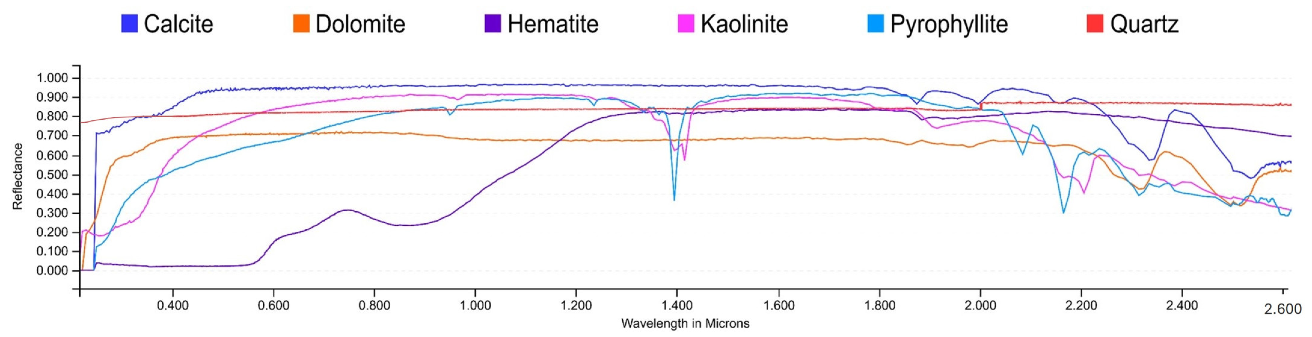
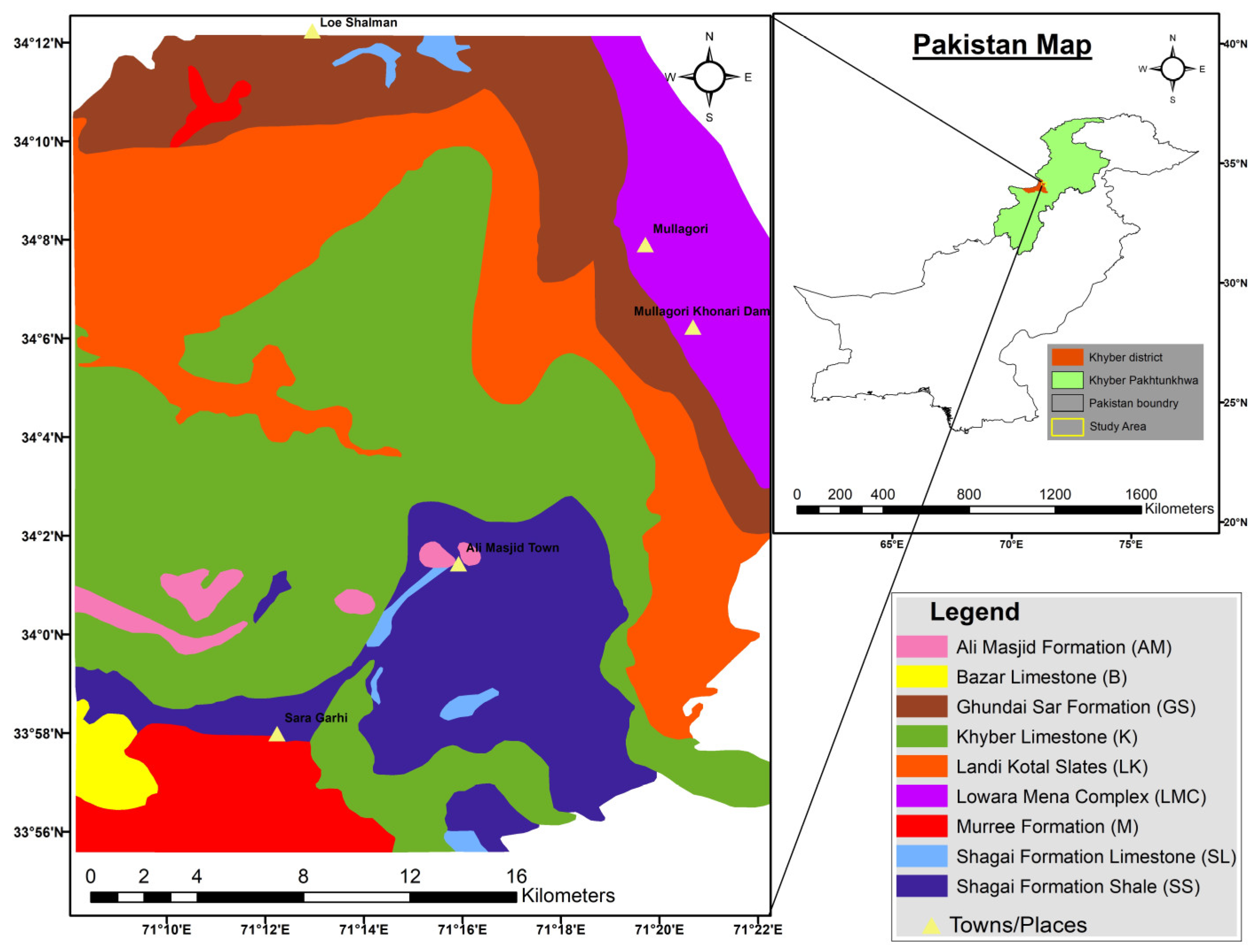
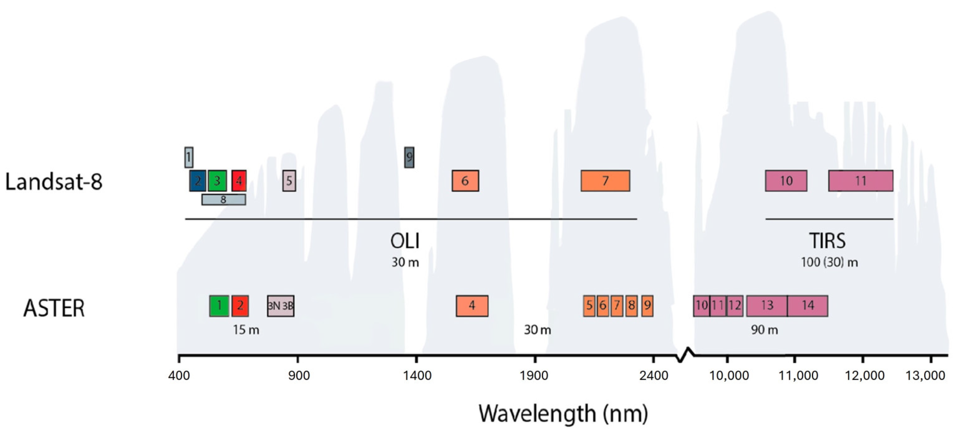
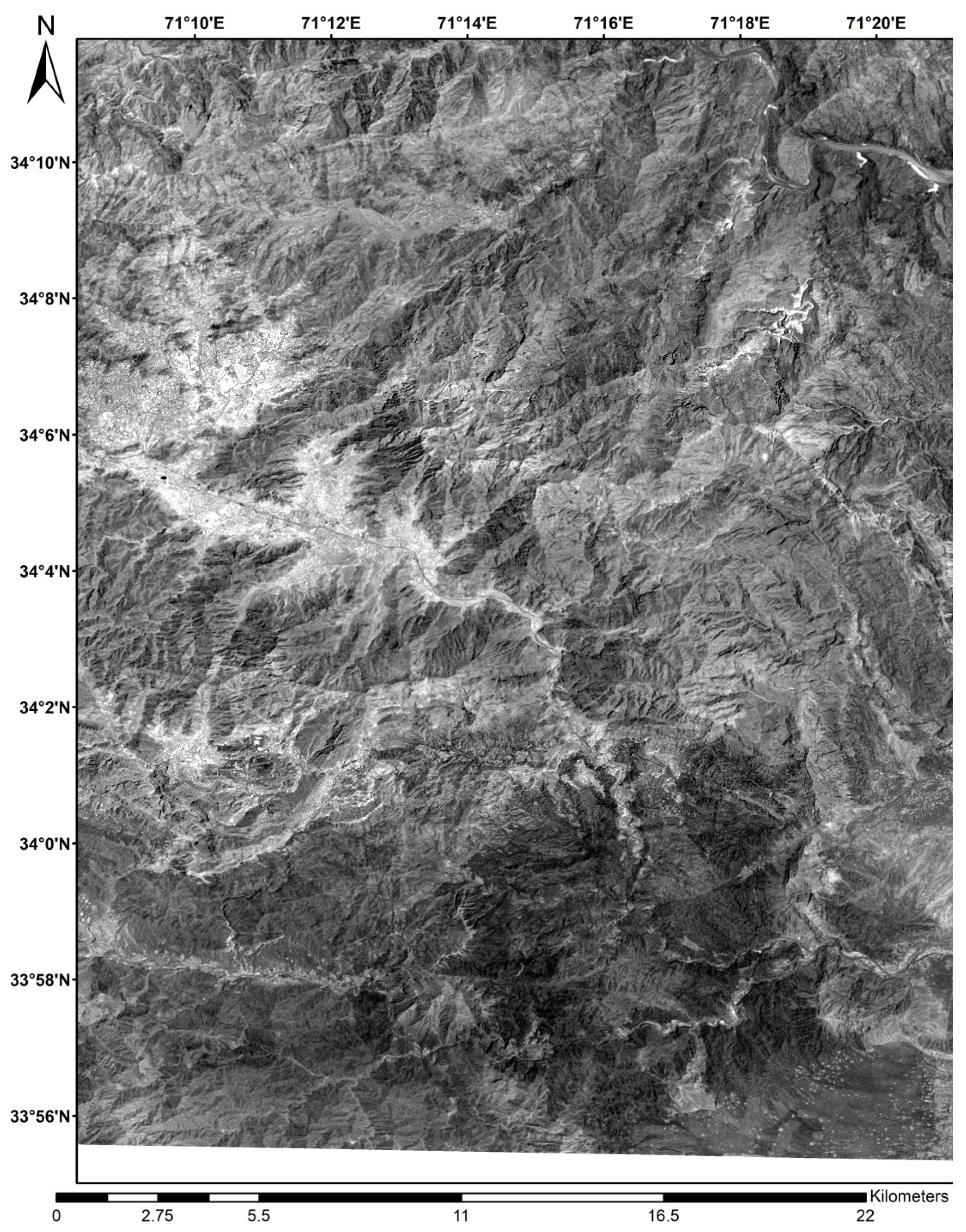
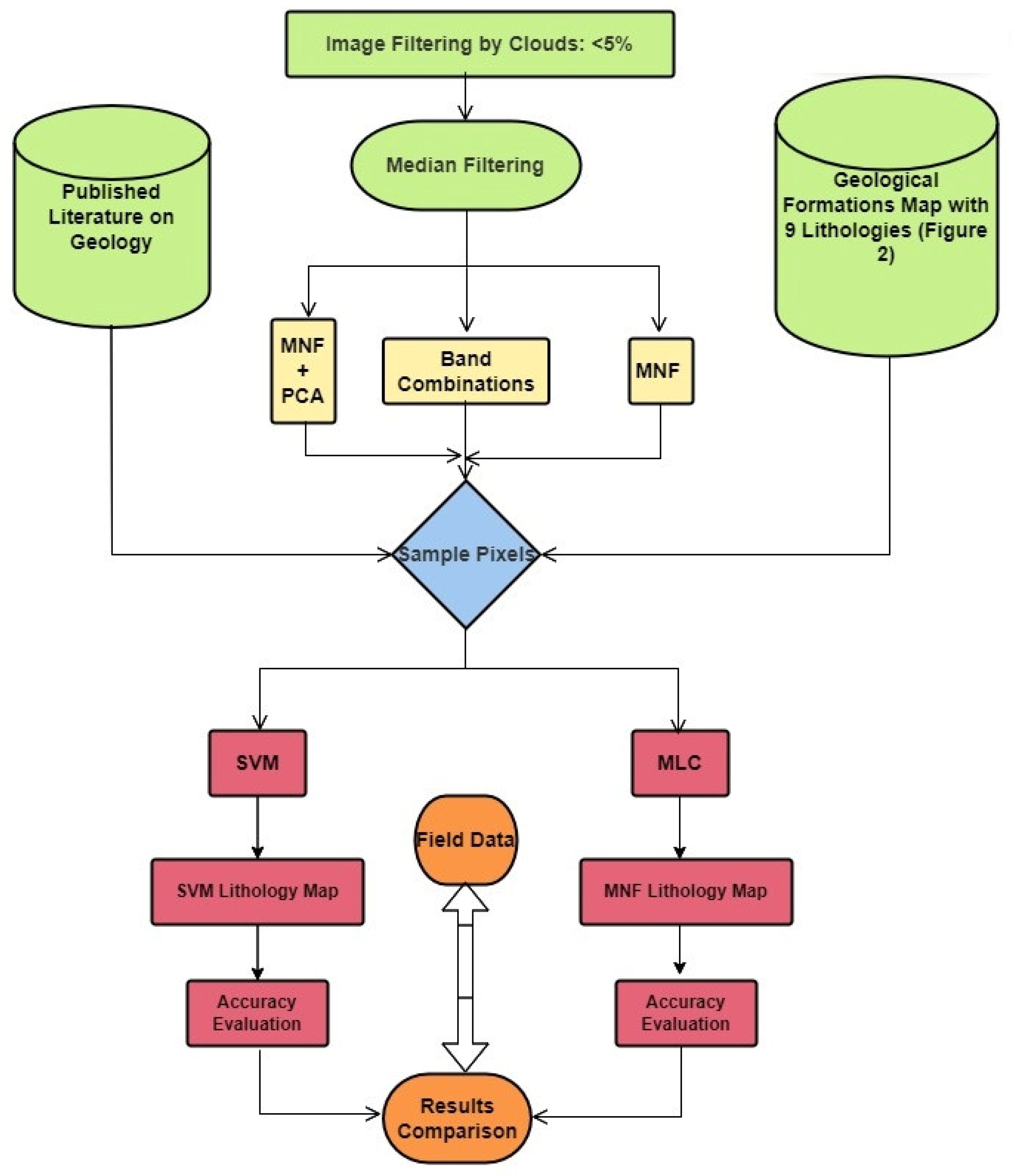
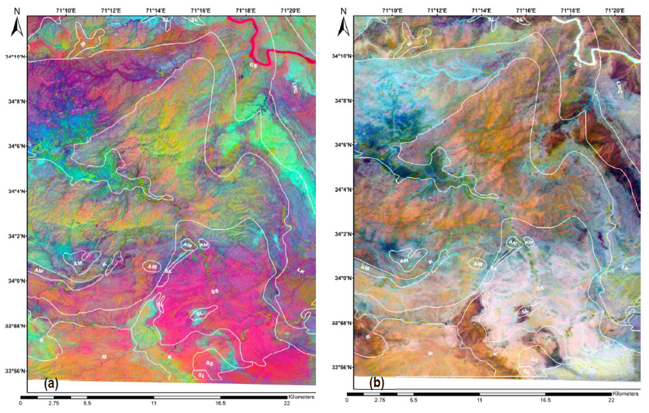
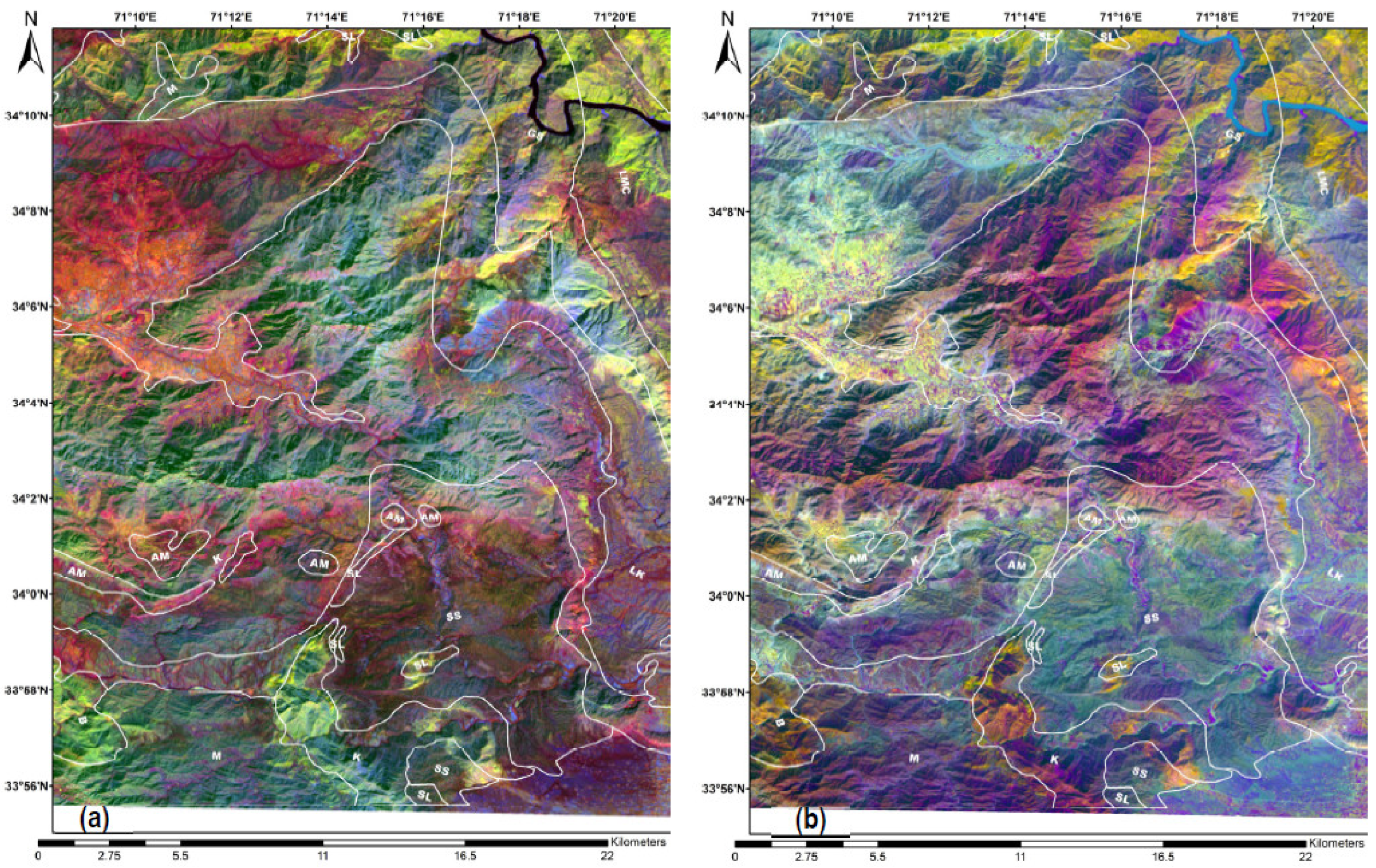
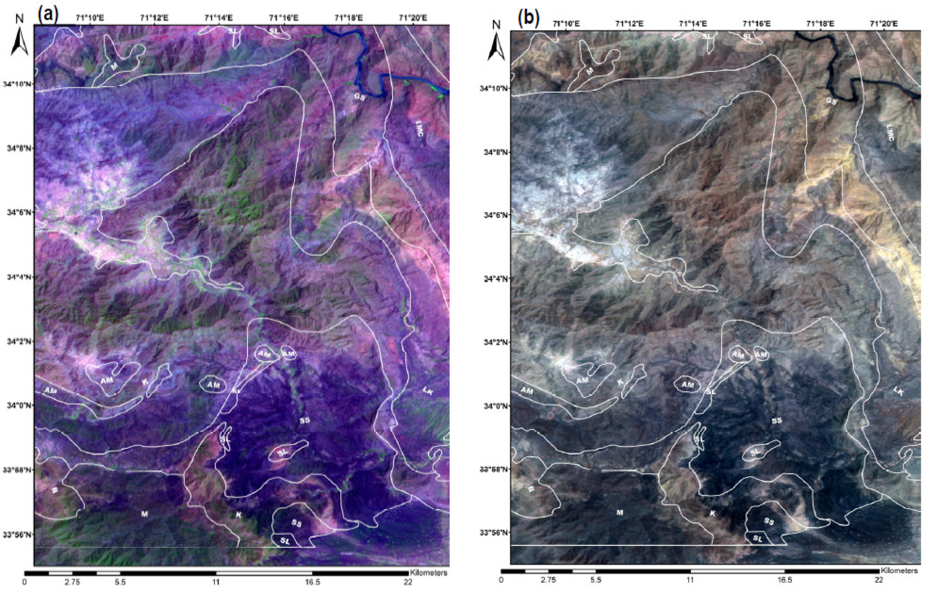
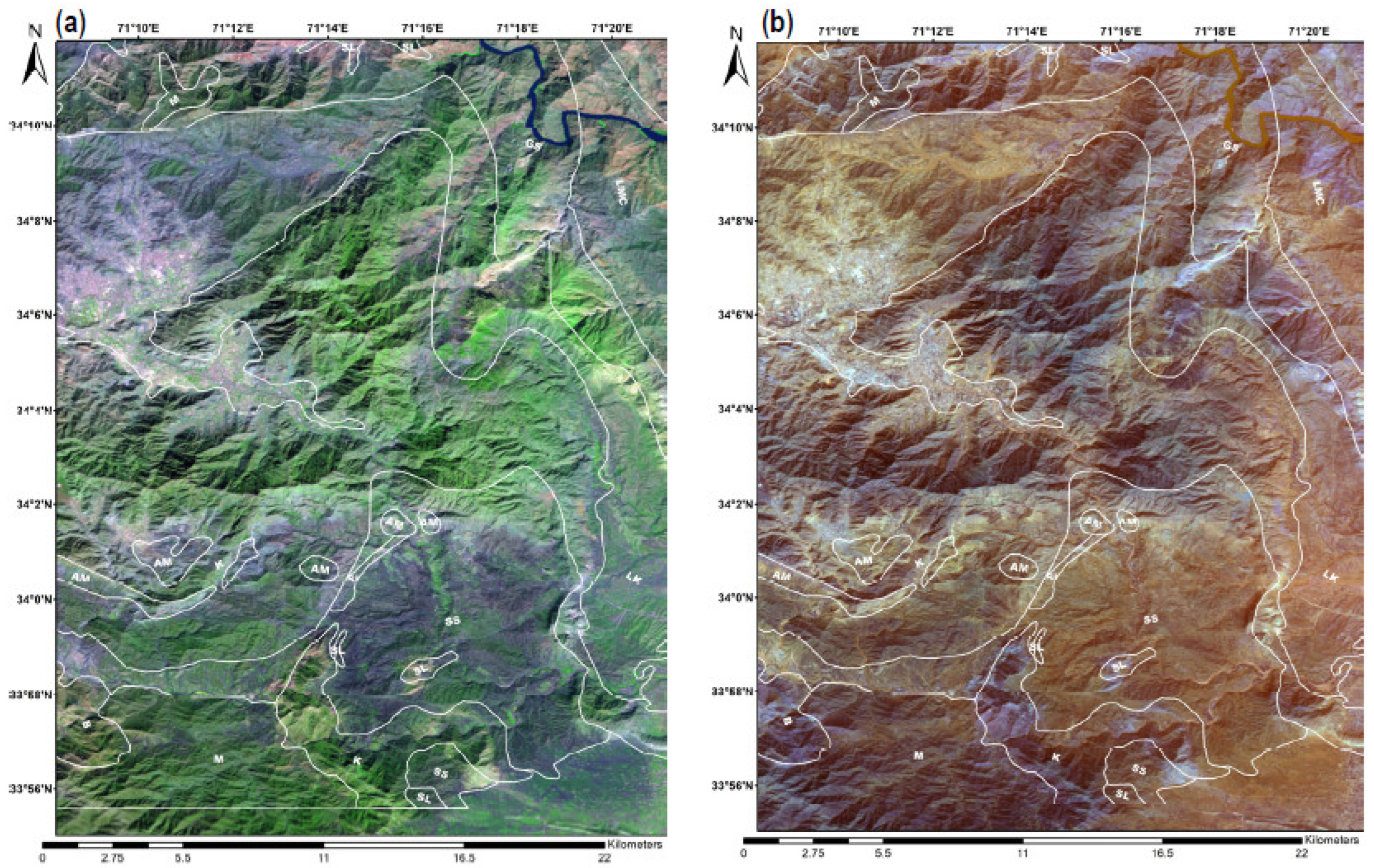

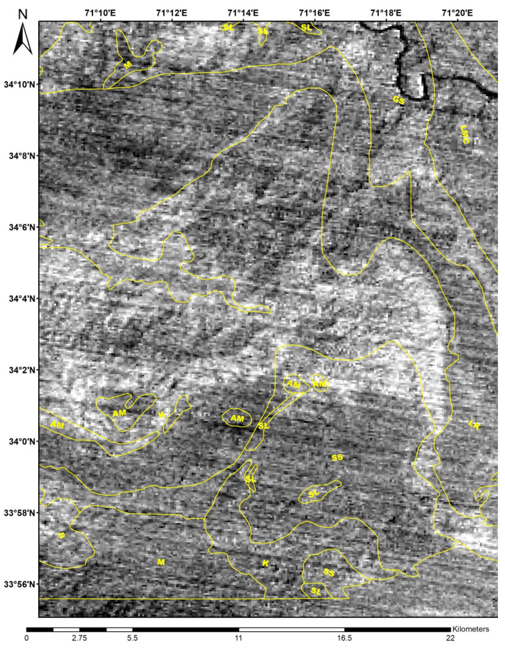
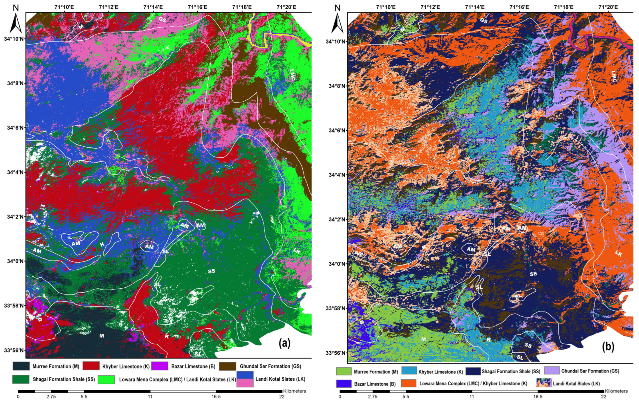


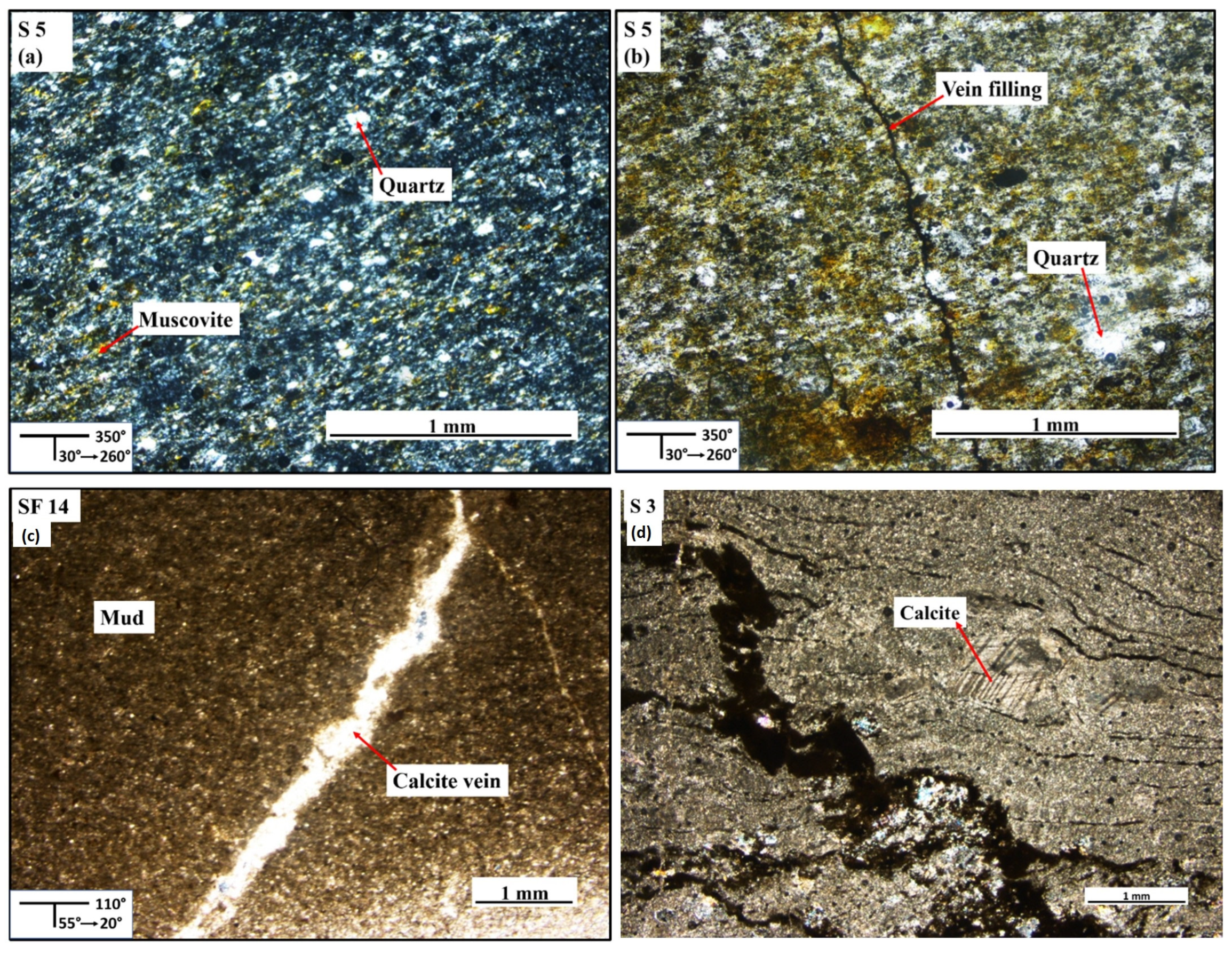
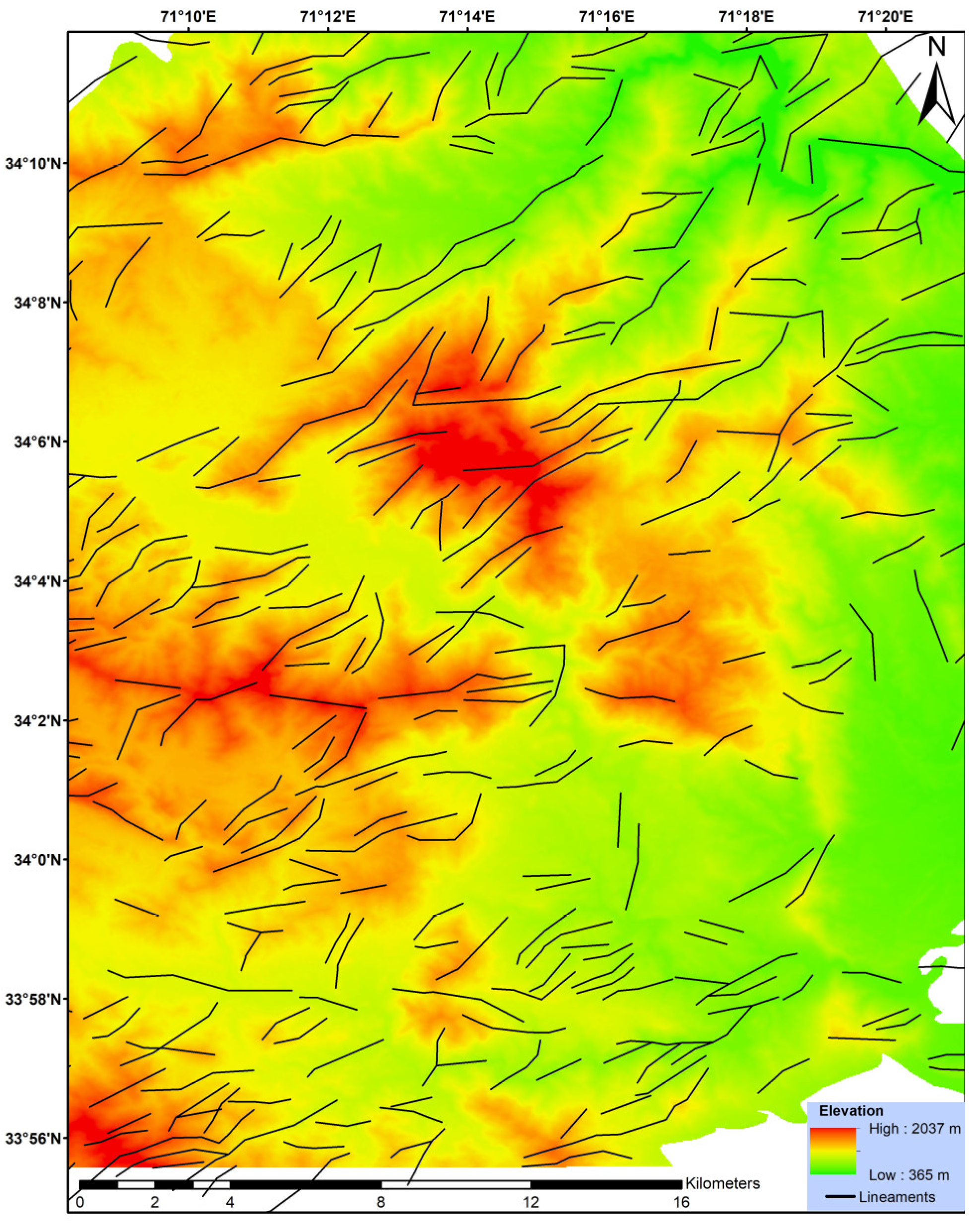
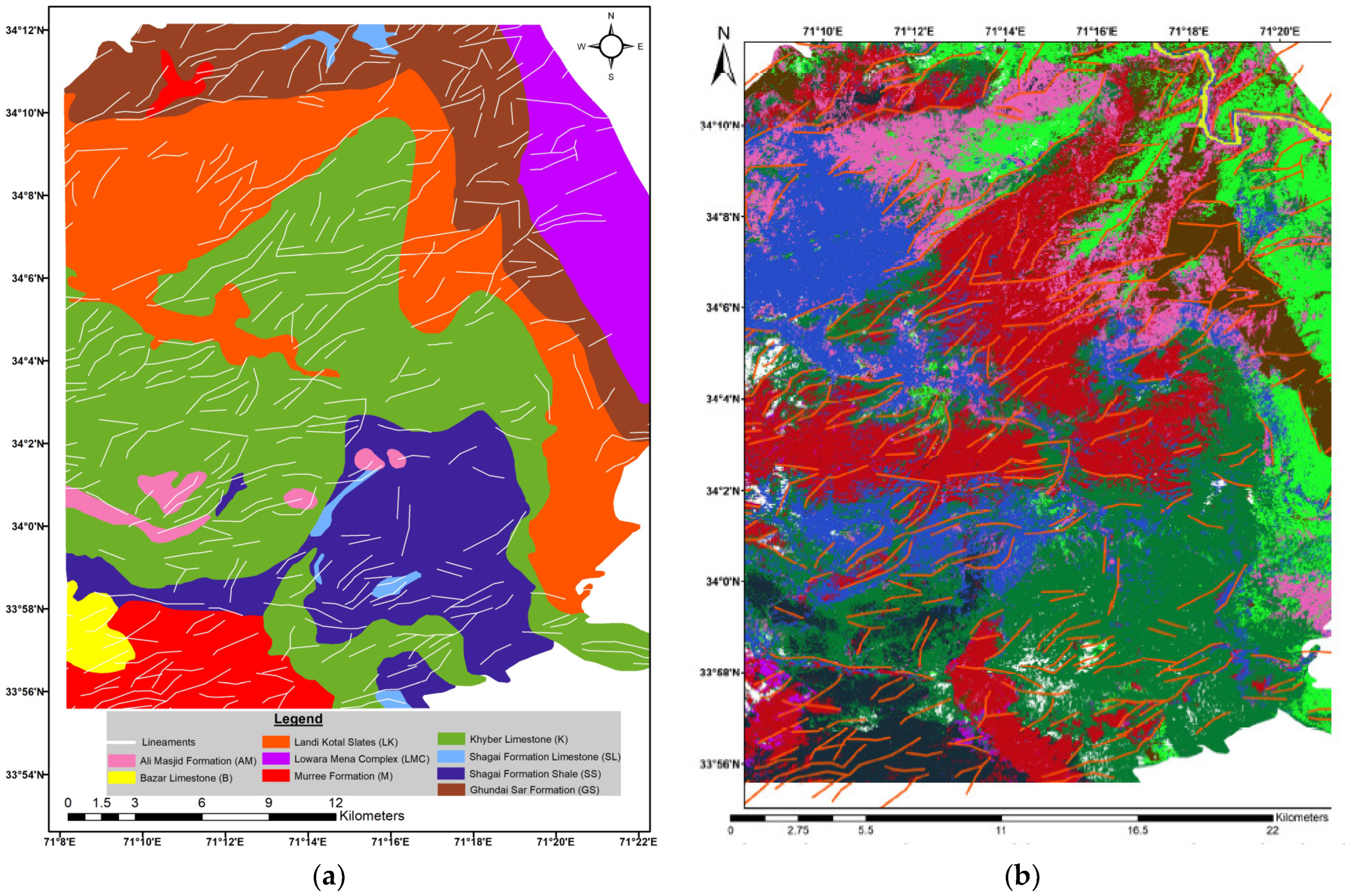
Disclaimer/Publisher’s Note: The statements, opinions and data contained in all publications are solely those of the individual author(s) and contributor(s) and not of MDPI and/or the editor(s). MDPI and/or the editor(s) disclaim responsibility for any injury to people or property resulting from any ideas, methods, instructions or products referred to in the content. |
© 2024 by the authors. Licensee MDPI, Basel, Switzerland. This article is an open access article distributed under the terms and conditions of the Creative Commons Attribution (CC BY) license (https://creativecommons.org/licenses/by/4.0/).