

Effects of Vertical Motion on Uplift of Underground Structure Induced by Soil Liquefaction

Department of Civil Engineering, National Chung Hsing University, Taichung 402, Taiwan
Appl. Sci. 2024, 14(12), 5098; https://doi.org/10.3390/app14125098
Submission received: 6 April 2024
/
Revised: 30 May 2024
/
Accepted: 4 June 2024
/
Published: 12 June 2024
(This article belongs to the Special Issue Seismic Resistant Analysis and Design for Civil Structures)
Abstract
:Featured Application
The conclusions of this article can be used to predict the uplift of tunnels or underground structures induced by soil liquefaction considering vertical earthquake motion.
Abstract
The uplift of underground structures induced by soil liquefaction can damage underground structure systems. Numerical simulations have shown that uplift is positively correlated with the energy of horizontal input motion. However, the effects of vertical input motion on uplift have not been studied comprehensively in the past. Previous studies on the vertical motion concluded that the effects of vertical motion on uplift depend on the overall characteristics of earthquake motion. These motion characteristics have only been studied separately in previous studies. A comprehensive study to explore the interactions and overall effects of these characteristics on the uplift of underground structures is essential. In this study, the FLAC program with the PM4Sand model was used as a numerical tool to explore the effects of vertical input motion on the uplift of underground structures. The numerical model was calibrated using centrifuge test results, and 48 earthquake motions were selected as input motions to study the effects of the overall characteristics of earthquake motions on the uplift of underground structures. The simulation results show that the frequency content characteristics of horizontal and vertical motion are the major factors affecting the uplift magnitude and the responses of liquefiable soils. However, most simulation cases show that the inclusion of vertical motion causes a 10% difference in the tunnel uplift, compared to cases without vertical motion.
1. Introduction
In modern society, it is preferred that lifelines and tunnels are built underground due to the need for space for construction in urban areas. Damage to these underground structures can lead to a great loss of lives and economic impacts. Therefore, the evaluation of the stability and safety of underground structure systems is essential. Earthquake hazards are the main cause of damage to underground structures. The liquefaction hazard is one of the hazards associated with earthquakes. The buoyancy force and the movement of liquefied soil from soil liquefaction initiate the uplift of underground structures. This uplift deformation could damage the connections between lifelines, causing leaks of hazardous liquids or gases. Moreover, damage to the connections in tunnels could endanger passengers in vehicles or trains. Uplift mechanisms and factors affecting the magnitude of uplift have been studied via model tests and numerical simulations in the past. Several studies [1,2,3,4,5,6,7,8,9,10,11] have observed that the magnitude of uplift is closely related to vertical and horizontal input motions.
Chou and Lin [8] used a numerical approach (the FLAC program with the UBCSAND model) to explore the effects of horizontal input motion on the magnitude of uplift. Their results showed that the magnitude of uplift and the Arias intensity (the energy of an earthquake) of input motion are positively correlated. Regarding vertical motion, in practice, the effects of vertical motion on uplift are not typically included in uplift predictions [1,12]. However, several studies have investigated the effects of vertical motion on uplift via numerical simulations. Liu and Song [2] used a strong-motion record from the Kobe earthquake and sinusoidal motion to study the effects of vertical motion on uplift. The numerical simulation results obtained by Liu and Song [2] showed that vertical motions cause an oscillation in excess pore pressure compared to cases without vertical motions, but the effects on uplift results are different. The vertical motion from the Kobe earthquake had a minimal effect on uplift magnitude, but the vertical motion of the sinusoidal motion significantly increased the uplift magnitude. Liu and Song [2] concluded that the effects of vertical motion on uplift depend on the overall characteristics of the motions. Bao et al. [6] used another strong motion record from the Kobe earthquake to study the effects of vertical motion on uplift magnitude. Their numerical simulation results showed that the magnitude of the uplift increases with the amplitude of the vertical motion. The effects of vertical input motions from the Kobe earthquake observed by Liu and Song [2] differed significantly from those observed by Bao et al. [6]. Huang [9] used the FLAC program with the UBCSAND model to study the effects of the amplitude, frequency, and phase angle of vertical motion on uplift using sinusoidal waves. The simulation results showed that the effects of these characteristics of vertical motion do not present obvious trends with uplift magnitude. The above studies on vertical motion provided insights into the effects of single characteristics (amplitude, frequency, or phase angle) of vertical motion on uplift. However, during the shaking caused by an earthquake, these characteristics occur randomly and interact with each other. Additionally, these studies provide only a few simulation results, which are insufficient for thoroughly exploring and determining the effects of vertical motion on uplift. Therefore, a comprehensive study to explore the overall effects of these characteristics on uplift is essential.
In this study, the FLAC program with the PM4Sand model [13,14,15,16,17] was selected as the numerical model to study the effects of vertical motion on uplift. This numerical model was first validated and calibrated using the centrifuge test results from Sasaki and Tamura [1]. As mentioned in the previous paragraph, earthquake motion characteristics interact with each other randomly during a shaking event. Therefore, in order to study the overall effects of earthquake motion characteristics on uplift, the approach typically used in previous studies (using the motion of one selected earthquake and adjusting one characteristic of this motion) is not appropriate. In this study, 48 sets of horizontal and vertical motions from 5 disastrous earthquake events in Taiwan were used as the input motions. This approach included all the characteristics and interactions between the characteristics of horizontal and vertical motions to comprehensively study the effects of vertical motion on the uplift.
2. PM4Sand Model
The PM4Sand model (version 3.1) [17] is based on the bounding surface plasticity model (DM model) proposed by Manzari and Dafalias [18] and Dafalias and Manzari [19], with modifications for geotechnical earthquake engineering applications. The PM4Sand model (version 3.1) is coded as a user-written constitutive model in FLAC 8.0 [20] with C++. The detailed descriptions and equations of the PM4Sand model (version 3.1) can be found in Boulanger and Ziotopoulou [17]. The main characteristics of the PM4Sand model (version 3.1) are summarized as follows:
- The PM4Sand model adopts the bounding, dilatancy, and critical state surfaces of the DM model but removes the Lode angle dependency proposed in the DM model to simplify the model calculation. The surfaces of the DM model in p–q space (p is the mean effective stress and q is the deviatoric stress) are shown in Figure 1.
- 2.
- The DM model incorporates the critical state behavior into the bounding and dilatancy surfaces by using the state parameter (the difference between the void ratio at the critical state and the current void ratio with the same mean effective stress). The PM4Sand model adopts the same concept but incorporates the relative state parameter index (the difference between the relative density at the critical state and the current relative density with the same mean effective stress). The critical state compatible bounding and dilatancy surfaces evolve when soil is sheared and will coincide with the critical state surface when the soil reaches the critical state. This concept allows the constitutive model to control the evolution of the peak friction angle according to the relative state of the soil during shearing.
- 3.
- The DM model includes the initial back–stress ratio (=q/p in p–q space) in the computation of the plastic modulus to account for the decrease in the plastic modulus with an increase in the back–stress ratio during loading. In the PM4Sand model, the initial back-stress ratio and the previous initial back-stress ratio are both tracked. In this way, the overestimated stiffening of the stress–strain response during the small unloading and reloading cycles in DM model can be improved.
- 4.
- The DM model uses the fabric–dilatancy tensor (z) to account for the build-up of porewater pressure upon the reversal of the stress increment following a dilative tendency response (the butterfly loop of the stress path) when the soil reaches soil liquefaction (at very low effective pressure). In the PM4Sand model, the total evolution of the fabric–dilatancy tensor is also tracked to control the rate of evolution for the fabric–dilatancy tensor and the plastic modulus. Thus, the undrained cyclic stress–strain response of the PM4Sand model can capture the progressively accumulated shear strains observed in the cyclic simple shear test which many plasticity models are not able to model. The responses of PM4Sand with two maximum fabric–dilatancy tensor values (zmax = 1 and 12) are plotted in Figure 2. Figure 2a shows the accumulated shear strain behavior during cyclic loading, and Figure 2b demonstrates that, through an adjustment of the value of zmax, the PM4Sand model can simulate the shape of a butterfly loop.
- 5.
- As the energy of the input motion is strongly related to the magnitude of the uplift [8], it is important to properly model the hysteretic response of the soil. The plastic modulus of the PM4Sand model is formulated to provide improved relationships of shear modulus reduction and equivalent damping ratio during drained cyclic loading. In addition, the elastic modulus of the PM4Sand model degrades with the total evolution of the fabric–dilatancy tensor to account for the progressive destruction with increasing plastic shear strains. This approach helps the PM4Sand model capture the hysteretic loop better than many plasticity models.
- 6.
- The key input parameters of the PM4Sand model (version 3.1) are listed and introduced in Table 1.
3. Numerical Model
The numerical model used in this study is the FLAC program with the PM4Sand model. FLAC is an explicit, finite difference program that performs Lagrangian analysis to calculate equilibrium equations and stress–strain relations. In the finite difference method (FDM), derivatives of governing equations of motion and constitutive relations are represented using physical variables (e.g., velocity and displacement) at discrete points (grid points in FLAC). The time−marching method is used in FLAC to solve these governing equations. The Lagrangian analysis updates the coordinates of the grid at each time step in the large strain mode of FLAC, which is most suitable for modeling the large deformations of soil induced by soil liquefaction.
The numerical model was validated and calibrated using the results of the centrifuge test studying the uplift of the underground structure [1]. The layout and monitored points of the numerical model are shown in Figure 3. Three centrifuge tests (listed in Table 2) were selected for numerical model verification and PM4Sand input parameter calibration. All tests consisted of one layer of Toyoura sand with different relative densities (Dr) and were subjected to a sinusoidal wave (20 cycles and 1.2 Hz). Time histories of six instruments (DV1, P2, PM2, PU1, A0, A2, and AM2, shown in Figure 3) in the centrifuge test CASE 98−01 were selected for comparison. The numerical model (shown in Figure 4) was composed of four sizes of FDM grids. The 0.5 m × 0.25 m and 0.5 m × 0.5 m (width × height) grids were placed around the underground structure to accurately capture the soil movement. The 1.0 m × 0.25 m and 1.0 m × 0.5 m grids were placed at areas away from the underground structure (1.5 times the width of the underground structure = 7.5 m) to lower the number of FDM grids and speed up the FLAC calculation. In this study, Toyoura sand was modeled using the PM4Sand model, and the underground structure was modelled as a rigid body using the elastic model with elastic moduli about 10 times the elastic moduli of Toyoura sand.
After evaluating the purposes of the key inputs of the PM4Sand model (listed in Table 1), three inputs were selected and adjusted to fit the centrifuge test results in this study: contraction rate parameter (hpo), ratio of plastic modulus to elastic modulus (ho), and material constant of bounding stress ratio (nb). hpo is one of the primary variables of the PM4Sand model used to adjust the contraction rates of the plastic volumetric strain. ho and nb are secondary variables of the PM4Sand model, which are used to adjust the ratio of plastic modulus to elastic modulus and to determine the slope of the bounding stress ratio. Other key inputs in this study follow the default values suggested by Boulanger and Ziotopoulou [17]. The calibrated input parameters for selected centrifuge tests are also listed in Table 3.
Time histories of monitoring points from the numerical simulation and the centrifuge test CASE98−01 are compared in Figure 5. A good match is found in the magnitude and trend of DV1 between the numerical simulation and the centrifuge test. Time histories of monitoring points P2 and A2, located in the free field, show that the amplitudes of the numerical simulation are slightly larger than those of the centrifuge test. This may be due to the fact that the dilatancy of the soil is overestimated by the PM4Sand model, leading to a higher acceleration oscillation in A2 and a higher pore pressure oscillation in P2. The excess pore pressure at PU1 from the numerical simulation was overestimated after 0.2 s. This could be due to the inability of the numerical model to capture the dilation of the soil caused by the uplift of the underground structure. The magnitudes of the oscillation of PM2 and AM2 were less than those from the centrifuge test, but the general trends are similar. The overall response of the numerical simulation was similar to that in the centrifuge test. Therefore, using the calibrated numerical model for further analyses of the vertical motion is reasonable.
4. Earthquake Motions
As explained earlier, earthquake motion is used as the input motion in this study to account for interactions between all characteristics of vertical motion. A total of 48 sets of vertical and horizontal motions (two sets of motions from one strong−motion station) from 5 disastrous earthquake events in Taiwan (listed in Table 4) were used in the numerical simulation. To include the magnitude and distance characteristics of vertical motion, selected sets of motions possess Mw = 5.8–7.6 and epicenter distance = 2 km–39 km. The wave propagation distance affects the high−frequency wave of the earthquake motion. To study the frequency content on the uplift, motions close to (2 km) and far away from (37 km) the epicenter were selected.
The comparisons of earthquake motion indices (peak acceleration; Arias intensity, Ia; and cumulative absolute velocity, CAV) in Figure 6 show that, in general, the energy of the vertical motion was less than that of the horizontal motion.
5. Results and Discussions
The calibrated numerical models with Dr = 30%, 50%, and 80% were subjected to selected sets of motions (both vertical and horizontal) to simulate the seismic response of the underground structure. To study the effects of vertical motion, simulation cases without vertical motion were performed for comparison. Figure 7 compares the uplifts of Dr = 30%, 50%, and 80% cases with and without vertical motion. The results show that most cases are located inside the 1.1:1.0 and 0.9:1.0 lines (uplift with vertical motion:uplift without vertical motion = UPVM:UP) with few exceptions (UPVM is much lower than UP).
In order to explore the relationship between the uplift and the vertical input motion, three characteristics (peak acceleration; Arias intensity, Ia; and cumulative absolute velocity, CAV) of both horizontal and vertical motions were used. The peak input acceleration is the most commonly used characteristic. In addition, results from Chou and Lin [8] showed that the magnitude of the uplift is positively correlated with the energy of the input motion. Therefore, Ia and CAV related to the energy of input motions were also used to explore the relationship between the uplift and the vertical input motion. Figure 8, Figure 9 and Figure 10 show the relationships between the uplift ratio (UPVM/UP) and three characteristics and ratios of three characteristics (peak input acceleration ratio = vertical peak input acceleration/horizontal pear input acceleration, Ia ratio = vertical Ia/horizontal Ia and CAV ratio = vertical CAV/horizontal CAV). The data points in these figures show that UPVM is much lower than UP when the vertical input motion has a higher peak acceleration, Ia, and CAV (the left plot of Figure 8, Figure 9 and Figure 10). However, no clear trends were found between uplift ratio and index ratios (the right plot of Figure 8, Figure 9 and Figure 10). Vertical input motions with high peak acceleration, Ia, and CAV mainly come from the Chi−Chi earthquake event.
In order to understand the real mechanisms of the vertical motion affecting the uplift magnitude, results and input motions of TCU071−N (the N−S direction of TCU071 motion), TCU063−N, and HWA027−N of Dr = 30% cases are plotted in Figure 11, Figure 12 and Figure 13. The intensity indices and uplift magnitudes for the TCU071−N, TCU063−N, and HWA027−N cases are listed in Table 5. TCU071−N represents the case where the vertical motion significantly lowers the uplift magnitude (>20%), TCU063−N represents the case where the vertical motion has a minor effect on the uplift magnitude (<5%), and HWA027−N represents the case where the vertical motion increases the uplift magnitude (>10%). Figure 11a, Figure 12a and Figure 13a show the time histories of the uplift with and without the vertical input motion. Excess pore pressure time histories of PM2 (located underneath the bottom of the structure) (Figure 11b, Figure 12b and Figure 13b) show that the inclusion of the vertical motion caused a transient response of the excess pore pressure for all cases. However, the amplitude and frequency of the transient response of the excess pore pressure in TCU071−N were significantly higher than those in TCU063−N and HWA027−N. As the transient response of the excess pore pressure is highly related to the input motion, the time histories of vertical motions and amplitudes of FFT of horizontal and vertical motions were also examined (Figure 11c,d, Figure 12c,d and Figure 13c,d). Comparisons show that TCU071−N had more high−frequency waves than TCU063−N and HWA027−N. In addition, amplitudes of FFT for the vertical motion were higher than those for the horizontal motion at different frequency ranges (TCU071−N at 9–14 Hz, TCU063−N at 0.2–0.3 Hz, and HWA027−N at 1.8 Hz).
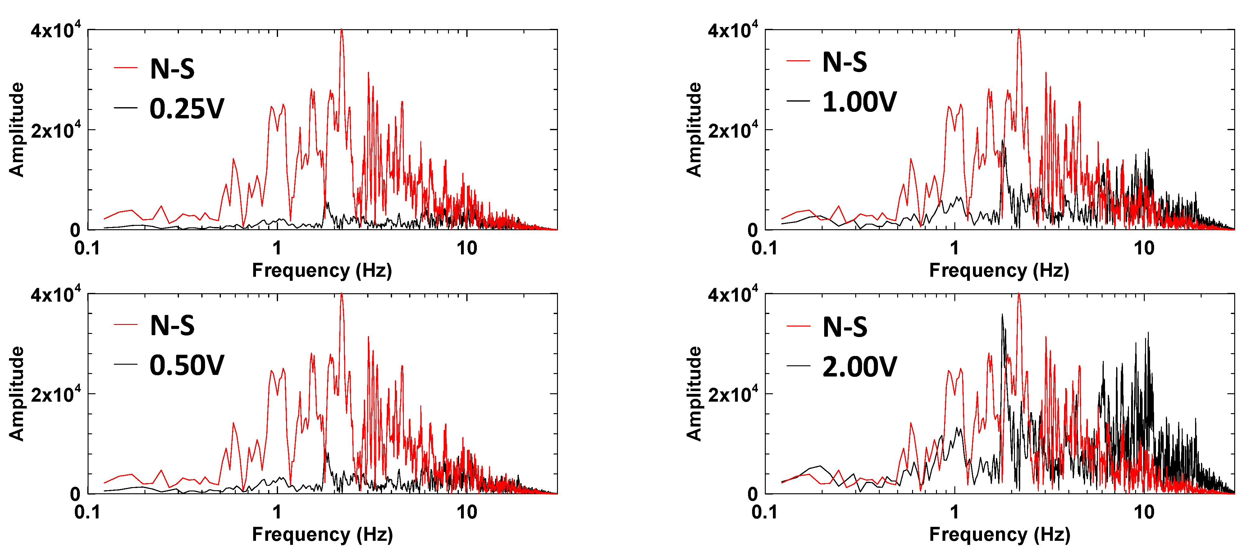
To understand the effects of the frequency content of the vertical motion comprehensively, additional simulations for TCU017−N and HWA027−N listed in Table 6 were performed. Figure 14 and Figure 15 compare the amplitude of FFT of input motions for different simulation cases. The observations are summarized as follows:
- A comparison of all TCU017−N cases shows that the decrease in the uplift is caused by the wave in the frequency range of 9–14 Hz in the vertical motion. When the amplitude of FFT in a frequency range of 9–14 Hz in the vertical motion is no longer higher than the amplitude of FFT at the same frequency range in the horizontal motion, the uplift ratio of TCU071−N cases increases from 0.77 in the 1.00 V case to 1.00 in the 0.33 V case.
- A comparison of the 2.00 V case of TCU071−N and all HWA027−N cases shows that the increase in the uplift is caused by the wave in the frequency range of 1–2 Hz (1.2 Hz for TCU071−N and 1.8 Hz for HWA027−N). When the amplitude of FFT at a frequency range of 1–2 Hz in the vertical motion is no longer higher than the amplitude of FFT in the same frequency range in the horizontal motion (0.33 V/0.66 V/1.00 V cases of TCU071−N and 0.25 V case of HWA027−N), the uplift ratio decreases.
- The predominant period, T, of the soil column in the centrifuge test is calculated as follows:where H is the height of the soil column in the centrifuge test (which is 10 m), and Vs is the shear wave velocity of the soil (as listed in Table 2). In this study, for Dr = 30% to 70%, T ranges from 0.31 s (4 × 10 m/130 m/s) to 0.2 s (4 × 10 m/200 m/s). The natural frequency of the soil column ranges from 3.22 Hz to 5 Hz. When soil is liquefied, the shear wave velocity of soil will decrease depending on the severity of the liquefaction, causing a decrease in the natural frequency of the soil column. Therefore, a possible explanation for the wave in the frequency range of 1–2 Hz increasing the uplift might be that this wave frequency range is close to the natural frequency of the liquefied soil. When the wave frequency range (9–14 Hz) is much higher than the natural frequency (3.22–5 Hz) of the soil column, these high frequency waves cause transient responses in the excess pore pressure and lower the uplift.T = 4 × H/Vs,
Liu and Song [2] and Bao et al. [6] used different Kobe earthquake motions to study the effects of vertical motion on uplift magnitude. Liu and Song [2] showed that the vertical motion has a minimal effect on uplift magnitude, but Bao et al. [6] showed that the magnitude of uplift increases with the amplitude of vertical motion. These observations show that the amplitude of vertical motion causes an increase or decrease in uplift depending on the frequency contents between the horizontal and vertical motions, not the amplitude of the vertical motion. This explains the different observations of Liu and Song [2] and Bao et al. [6].
6. Conclusions
In this study, the effects of vertical motion on the uplift of underground structures induced by soil liquefaction were explored via a numerical simulation approach using the FLAC program with the PM4Sand model. The PM4Sand model is modified from the bounding surface plasticity model to model behaviors of liquefiable soils for geotechnical earthquake engineering applications. The numerical model was first verified and calibrated using centrifuge tests from Sasaki and Tanura [1] for soil layers with Dr = 30%, 50%, and 80%. Then, the effects of vertical motion were studied using 48 ground motion time histories from 5 earthquake events. The simulation results showed that the vertical motion could cause an increase, decrease, or negligible change in the uplift. Additional simulations of TCU071−N and HWA027−N cases showed that the variation in the peak acceleration amplitude causes an increase or a decrease in the uplift depending on frequency contents between the horizontal and vertical motions. This observation effectively explains the contrary results of Liu and Song [2] and Bao et al. [6]. The effects of the vertical motion on the uplift are summarized as follows:
- Most simulation cases with vertical input motion have uplift ratios between 0.9 and 1.1 (a 10% difference in the uplift). Exceptions are cases where the vertical motion lowers the uplift by 20% to 50%. These exceptions occur in cases with higher peak acceleration, Arias intensity, and CAV. These cases come from the Chi−Chi earthquake event, which possessed a higher earthquake magnitude.
- If the amplitude of FFT of the vertical motion is higher than the amplitude of FFT of the horizontal motion at a frequency range higher (twice as high) than the natural frequency of soil, then, the vertical motion decreases the uplift. Conversely, if the amplitude of FFT of the vertical motion is higher than the amplitude of FFT of the horizontal motion in a frequency range close to the natural frequency of soil, then the vertical motion increases the uplift.
For a preliminary calculation without a numerical simulation, the uplift with the vertical motion can be estimated conservatively using 1.1 times the uplift without the vertical motion. However, the effects of the vertical motion on the uplift in this study were based on the numerical simulation results only. These observations still need to be verified through a model test (the centrifuge test or the shaking table test).
Funding
This research is funded by National Science and Technology Council, Taiwan, R.O.C. under grant no. 109-2221-E-005-007-MY3.
Institutional Review Board Statement
Not applicable.
Informed Consent Statement
Not applicable.
Data Availability Statement
The datasets generated during and/or analyzed during the current study are available from the corresponding author on reasonable request.
Acknowledgments
I like to thank the National Center for Research on Earthquake Engineering (NCREE) for providing the catalog of earthquake motions.
Conflicts of Interest
The authors declare no conflicts of interest.
References
- Sasaki, T.; Tamura, K. Prediction of liquefaction-induced uplift displacement of underground structures. In Proceedings of the 36th Joint Meeting US-Japan Panel on Wind and Seismic Effects, Gaithersburg, MD, USA, 17–22 May 2004; Volume 36, pp. 191–198. [Google Scholar]
- Liu, H.; Song, E. Seismic response of large underground structures in liquefiable soils subjected to horizontal and vertical earthquake excitations. Comput. Geotech. 2005, 32, 223–244. [Google Scholar] [CrossRef]
- Chou, J.C. Centrifuge Modeling of the BART Transbay Tube and Numerical Simulation of Tunnels in Liquefying Ground. Ph.D. Dissertation, University of California, Davis, CA, USA, 2010. [Google Scholar]
- Madabhushi, S.S.C.; Madabhushi, S.P.G. Finite element analysis of floatation of rectangular tunnels following earthquake induced liquefaction. Indian Geotech. J. 2015, 45, 233–242. [Google Scholar] [CrossRef]
- Han, Y.; Liu, H. Failure of circular tunnel in saturated soil subjected to internal blast loading. Geomech. Eng. 2016, 11, 421–438. [Google Scholar] [CrossRef]
- Bao, X.; Xia, Z.; Ye, G.; Fu, Y.; Su, D. Numerical analysis on the seismic behavior of a large metro subway tunnel in liquefiable ground. Tunn. Undergr. Space Technol. 2017, 66, 91–106. [Google Scholar] [CrossRef]
- Castiglia, M.; de Magistris, F.S.; Napolitano, A. Stability of onshore pipelines in liquefied soils: Overview of computational methods. Geomech. Eng. 2018, 14, 355–366. [Google Scholar] [CrossRef]
- Chou, J.C.; Lin, D.G. Incorporating ground motion effects into Sasaki and Tamura prediction equations of liquefaction-induced uplift of underground structures. Geomech. Eng. 2020, 22, 25–33. [Google Scholar] [CrossRef]
- Huang, K.H. Effects of Vertical Motion on Liquefaction-Induced Uplift of Underground Structure. Master’s Thesis, National Chung Hsing University, Taichung, China, 2021. (In Chinese). [Google Scholar]
- Do, T.M.; Do, A.N.; Vo, H.T. Numerical analysis of the tunnel uplift behavior subjected to seismic loading. J. Min. Earth Sci. 2022, 63, 1–9. [Google Scholar]
- Wang, R.; Zhu, T.; Yu, J.K.; Zhang, J.M. Influence of vertical ground motion on the seismic response of underground structures and underground-aboveground structure systems in liquefiable ground. Tunn. Undergr. Space Technol. 2022, 122, 104351. [Google Scholar] [CrossRef]
- Seyedi, M. An Empirical Function to Predict the Liquefaction-Induced Uplift of Circular Tunnels. Transp. Infrastruct. Geotech. 2024, 1–26. [Google Scholar] [CrossRef]
- Boulanger, R.W. A Sand Plasticity Model for Earthquake Engineering Applications; Center for Geotechnical Modeling: Davis, CA, USA, 2010. [Google Scholar]
- Boulanger, R.W.; Ziotopoulou, K. Formulation of a sand plasticity plane-strain model for earthquake engineering applications. J. Soil Dyn. Earthq. Eng. 2013, 53, 254–267. [Google Scholar] [CrossRef]
- Ziotopoulou, K.; Boulanger, R.W. Calibration and implementation of a sand plasticity plane-strain model for earthquake engineering applications. J. Soil Dyn. Earthq. Eng. 2013, 53, 268–280. [Google Scholar] [CrossRef]
- Ziotopoulou, K.; Boulanger, R.W. Plasticity modeling of liquefaction effects under sloping ground and irregular cyclic loading conditions. Soil Dyn. Earthq. Eng. 2016, 84, 269–283. [Google Scholar] [CrossRef]
- Boulanger, R.W.; Ziotopoulou, K. PM4Sand (Version 3.1): A Sand Plasticity Model for Earthquake Engineering Applications; Department of Civil and Environmental Engineering, University of California: Davis, CA, USA, 2017. [Google Scholar]
- Manzari, M.T.; Dafalias, Y.F. A critical state two-surface plasticity model for sands. Géotechnique 1997, 47, 255–272. [Google Scholar] [CrossRef]
- Dafalias, Y.F.; Manzari, M.T. Simple plasticity sand model accounting for fabric change effects. J. Eng. Mech. 2004, 130, 622–634. [Google Scholar] [CrossRef]
- FLAC Version 8.0, Itasca Consulting Group Inc.: Minneapolis, MN, USA, 2016.
- Andrus, R.D.; Stokoe, K.H. Liquefaction resistance of soils from shear-wave velocity. J. Geotech. Geoenviron. Eng. ASCE 2000, 126, 1015–1025. [Google Scholar] [CrossRef]
- Itasca UDM Web Site. Available online: https://www.itascacg.com/software/udm-library/ubcsand (accessed on 1 October 2023).
Figure 1.
Demonstration of surfaces of the bounding surface plasticity model (modified from Dafalias and Manzari [19]).
Figure 1.
Demonstration of surfaces of the bounding surface plasticity model (modified from Dafalias and Manzari [19]).

Figure 2.
Responses of cyclic undrained simple shear test of PM4Sand model: (a) shear stress and shear strain and (b) stress path.
Figure 2.
Responses of cyclic undrained simple shear test of PM4Sand model: (a) shear stress and shear strain and (b) stress path.
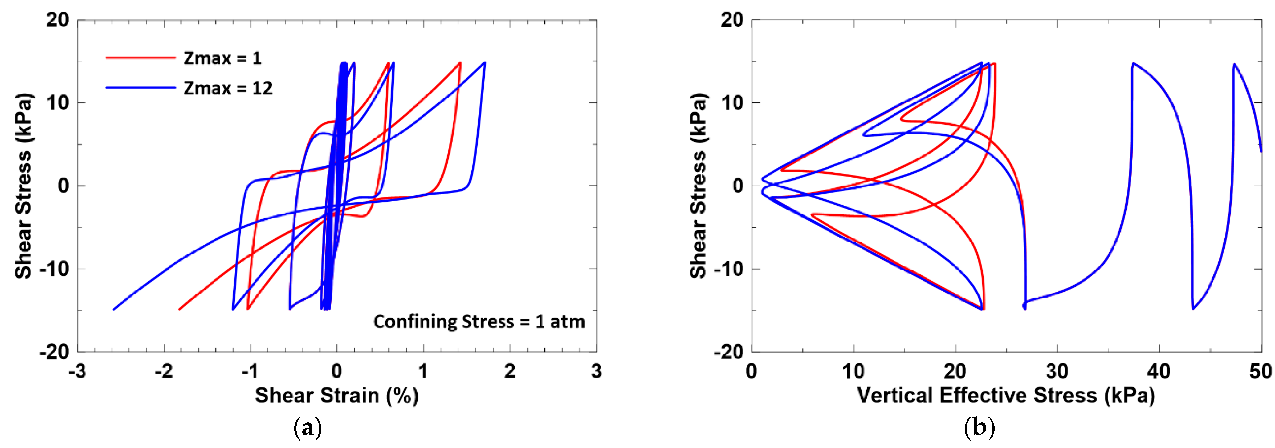
Figure 3.
Dimensions and monitoring points of the numerical model.
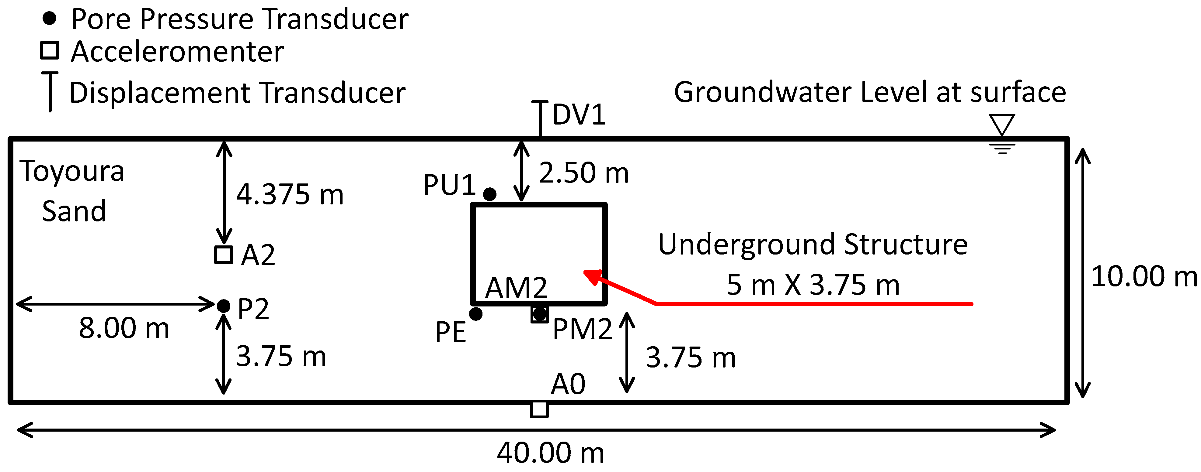
Figure 4.
FLAC grids of the numerical model.
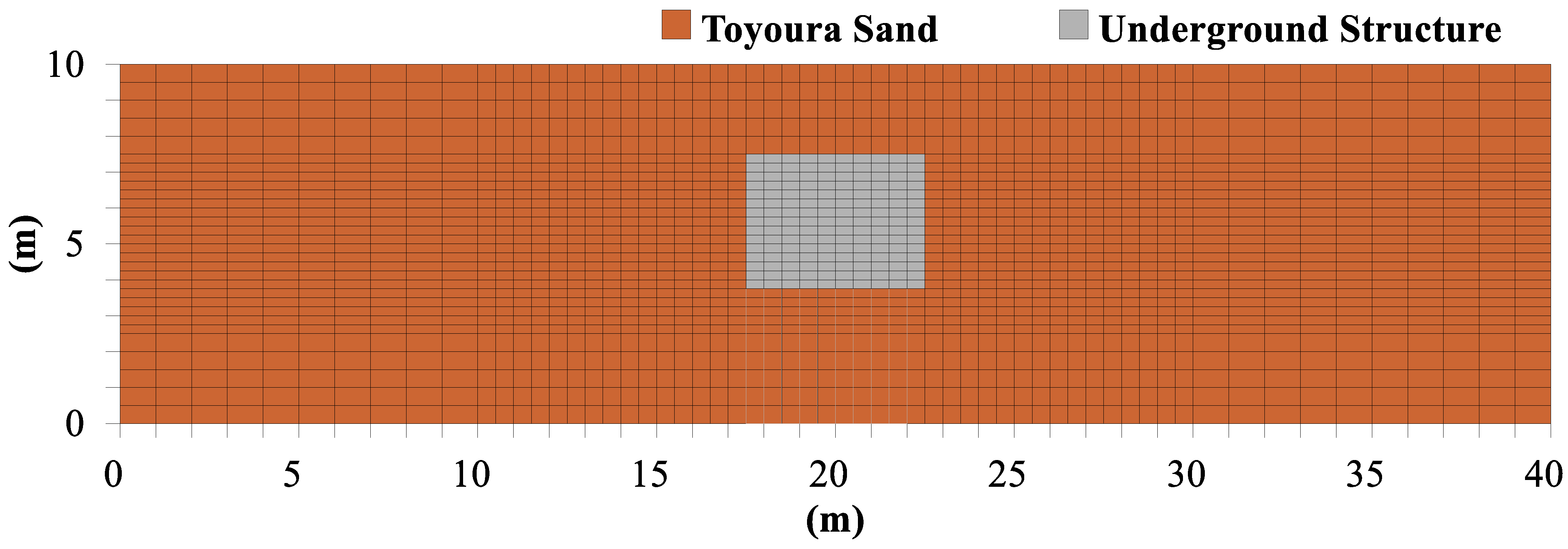
Figure 5.
Comparisons of centrifuge test and simulation results (modified from [1]).
Figure 5.
Comparisons of centrifuge test and simulation results (modified from [1]).

Figure 6.
Comparisons of earthquake motion indices: (a) peak acceleration; (b) Arias intensity; and (c) cumulative absolute velocity.
Figure 6.
Comparisons of earthquake motion indices: (a) peak acceleration; (b) Arias intensity; and (c) cumulative absolute velocity.
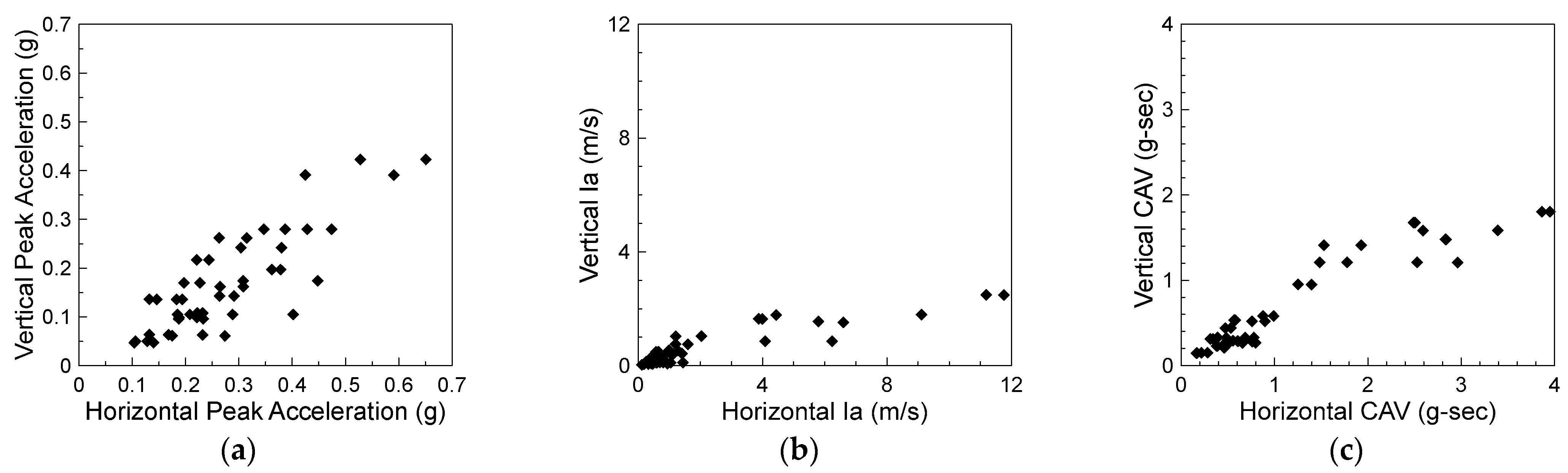
Figure 7.
Comparisons of uplifts with and without vertical motions.
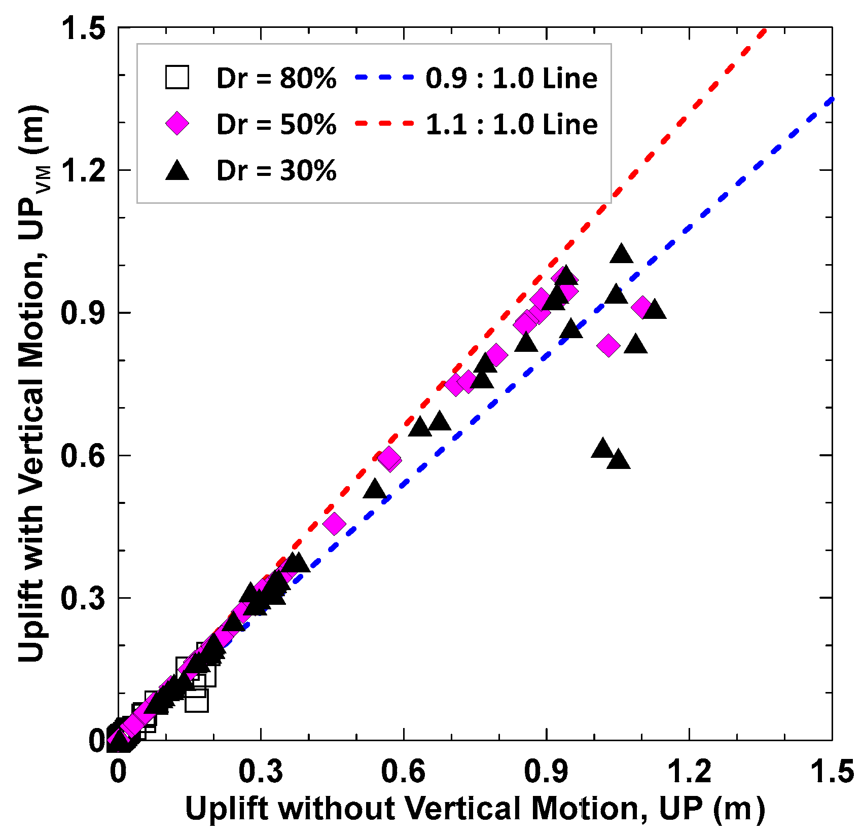
Figure 8.
Uplift ratio vs. vertical peak input acceleration and peak input acceleration ratio.
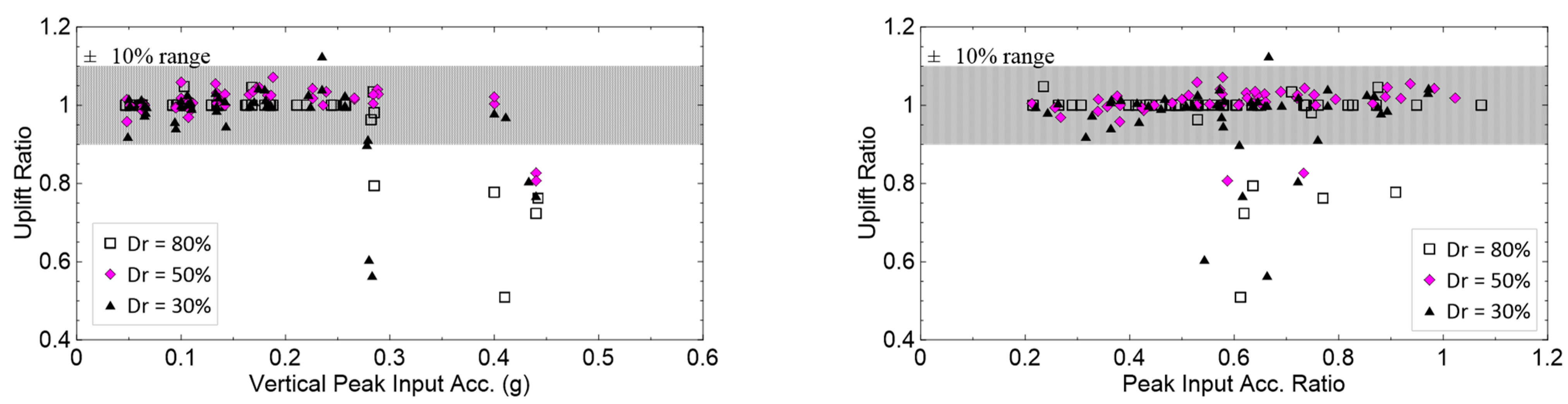
Figure 9.
Uplift ratio vs. Ia of vertical motion and Ia ratio.
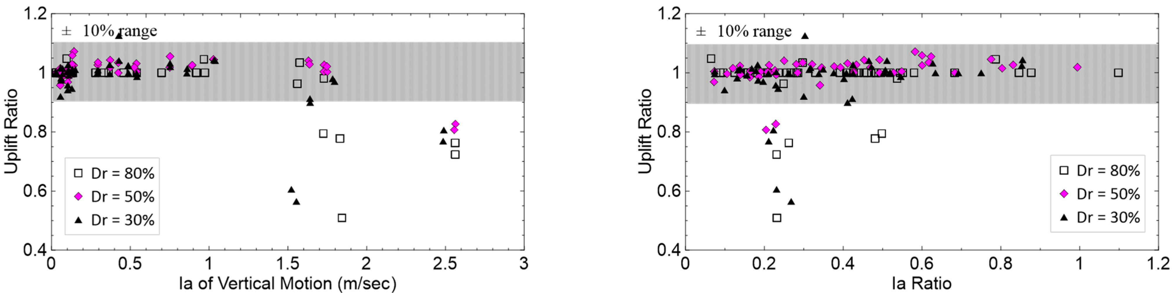
Figure 10.
Uplift ratio vs. CAV of vertical motion and CAV ratio.

Figure 11.
Time histories and FFT of TCU071−N case.
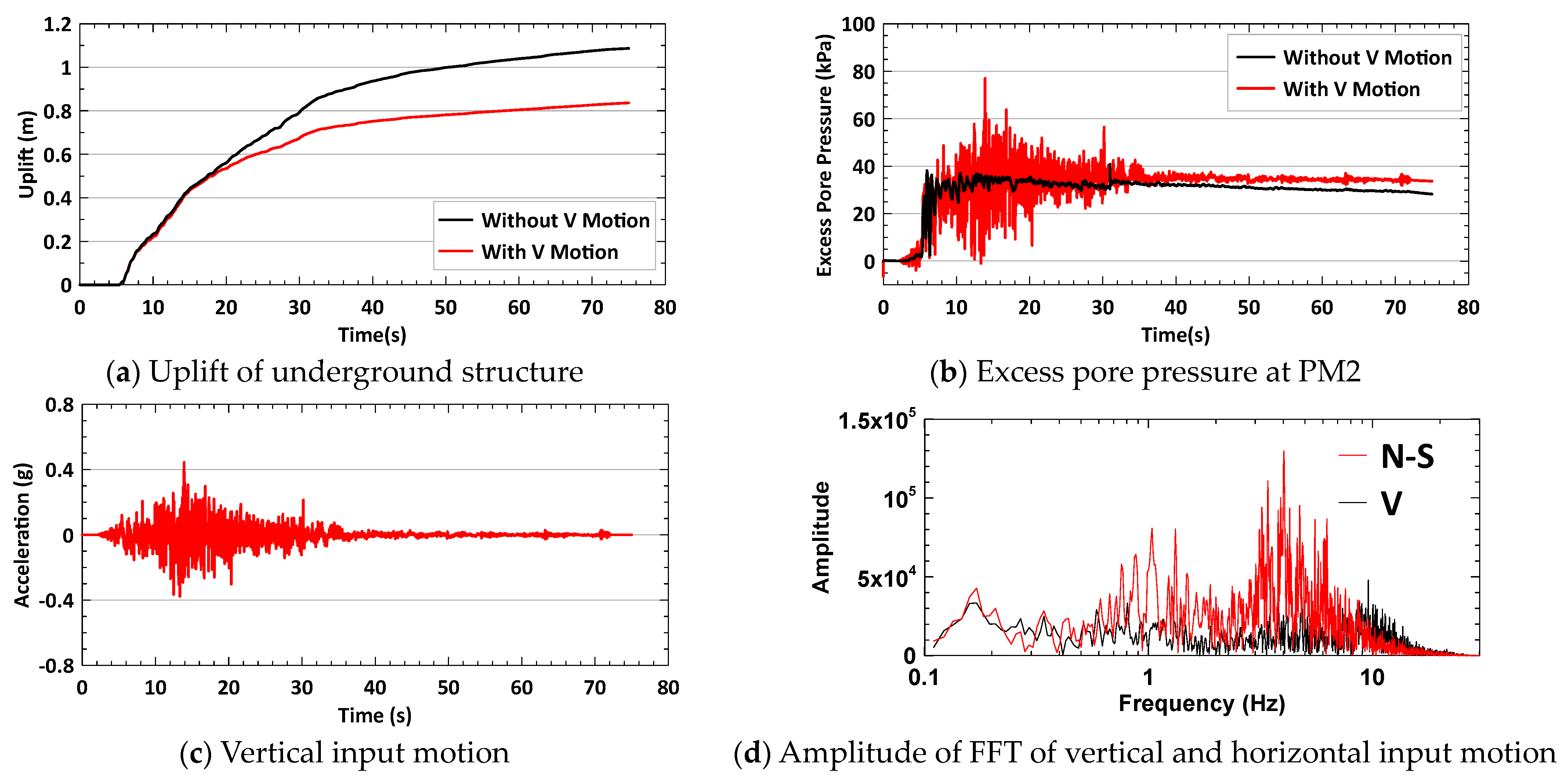
Figure 12.
Time histories and FFT of TCU063−N case.
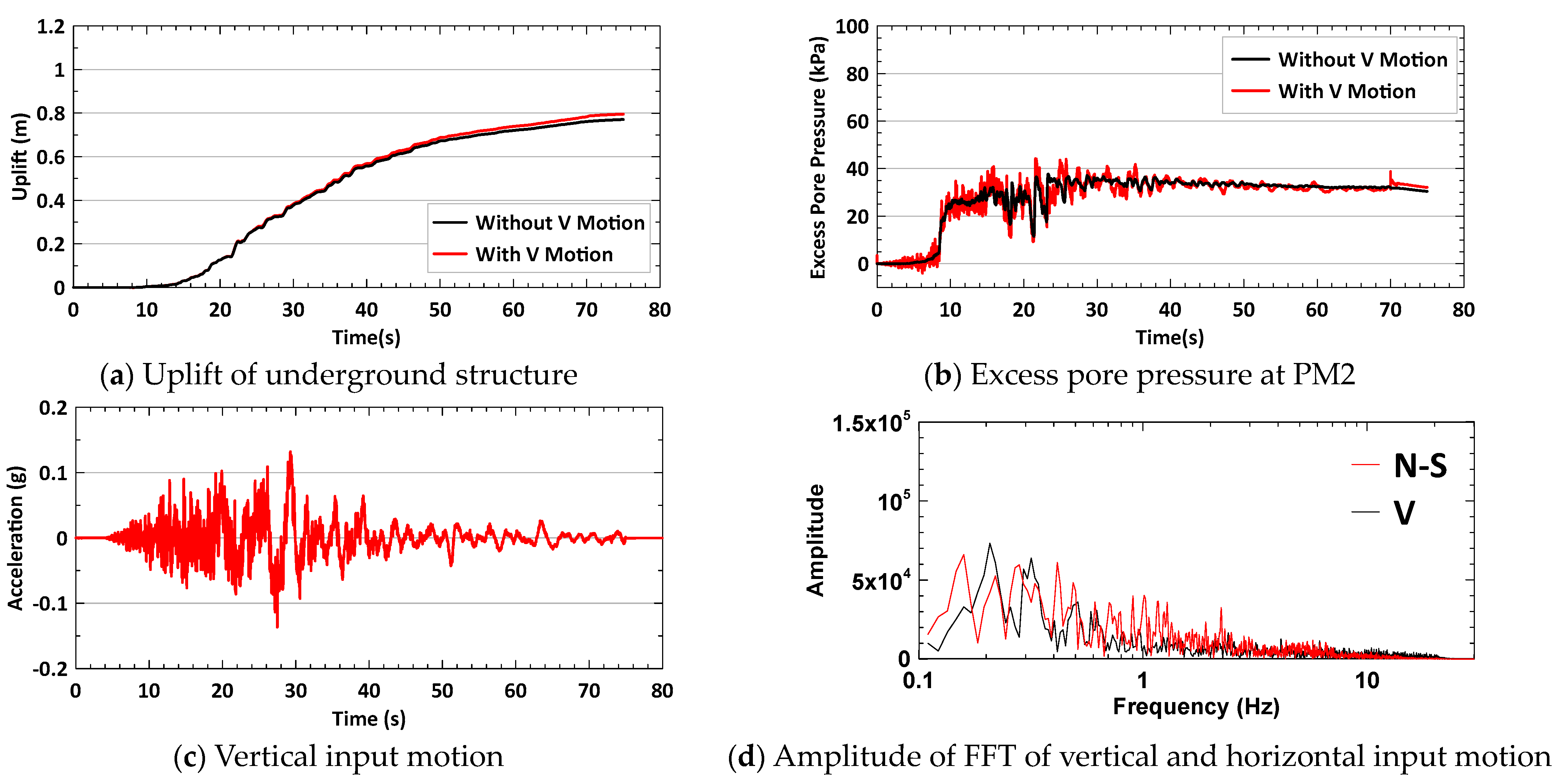
Figure 13.
Time histories and FFT of HWA027−N case.
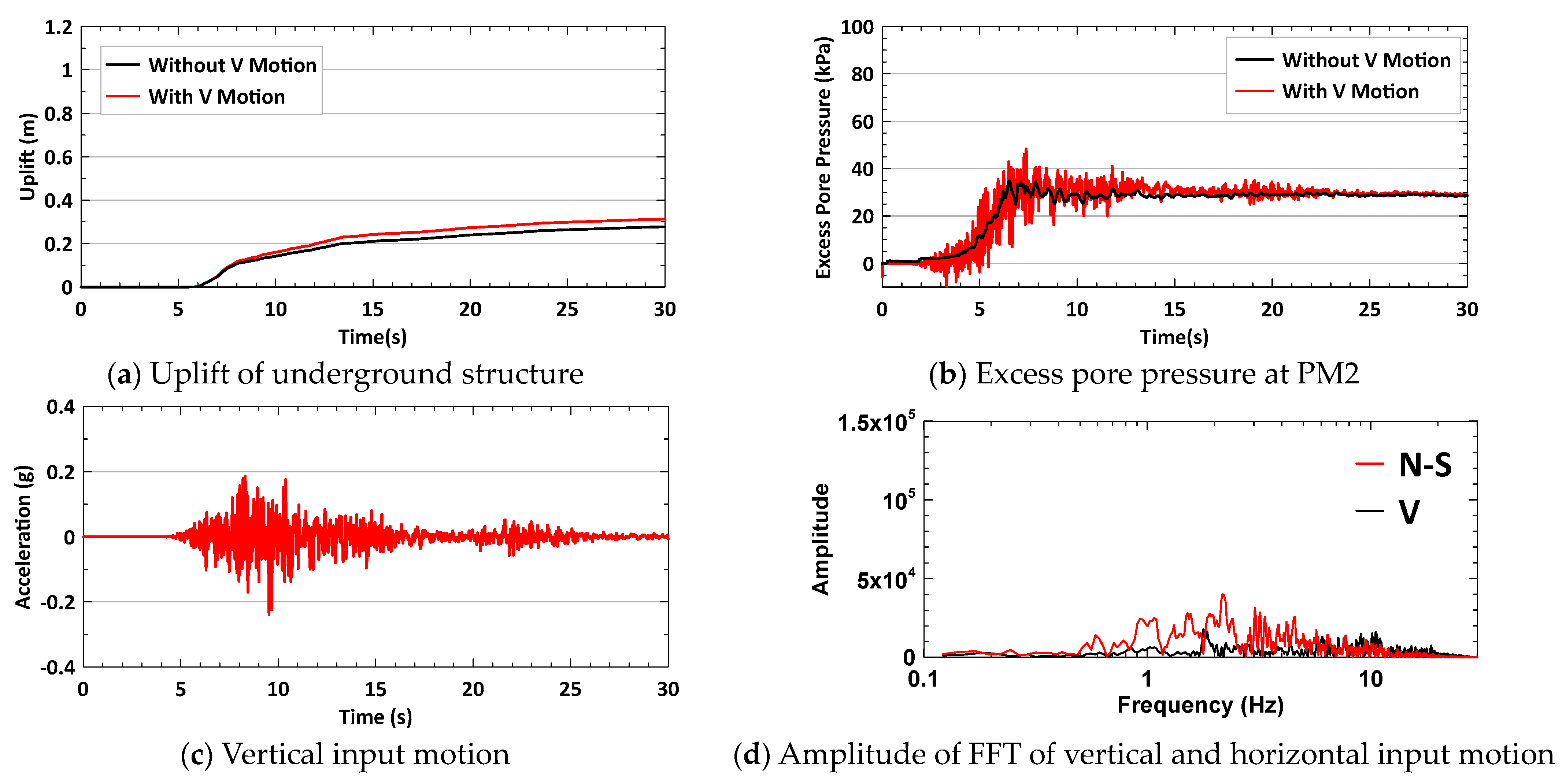
Figure 14.
Comparisons of amplitude of FFT for additional TCU071−N cases.

Figure 15.
Comparisons of amplitude of FFT for additional HWA027−N cases.

Table 1.
Key input parameters of the PM4Sand model.
| Input Parameter | Description |
|---|---|
| Shear modulus coefficient (Go) | Go is used to estimate the small strain shear modulus. |
| Contraction rate parameter (hpo) | hpo controls the contraction rate of the plastic volumetric strain related to the cyclic resistance ratio (CRR) of soil. |
| Ratio of plastic modulus and elastic modulus (ho) | ho relates to relative density (Dr) and controls the ratio of plastic modulus to elastic modulus. Model default value provides reasonable modulus reduction and damping curves. |
| Material constant of bounding stress ratio (nb) | nb controls the bounding surface (dilatancy), which is related to the peak effective friction angles. |
| Material constant of dilatancy stress ratio (nd) | nd controls the phase transformation where the contraction behavior transitions to the dilation behavior. |
| Maximum value of fabric–dilatancy tensor (zmax) | zmax is the maximum value of fabric–dilatancy tensor. |
| Material constant of dilatancy (Ado) | zmax and Ado are used to control the buildup value of the porewater pressure upon reversal of stress increment following a dilative tendency response. |
Table 2.
Centrifuge test information.
| Centrifuge Test Case No | 97−06 | 98−01 | 97−02 |
|---|---|---|---|
| Unit weight of underground structure | 0.8 t/m3 | 0.8 t/m3 | 0.8 t/m3 |
| Relative density of Toyoura sand (Dr) | 30% | 50% | 80% |
| Equivalent SPT N value, (N1)60 1 | 4 | 12 | 30 |
| Shear wave velocity (Vs) 2 | 130 m/s | 165 m/s | 200 m/s |
| Input motion | Sinusoidal wave (20 cycles with 1.2 Hz) | ||
| Uplift of centrifuge test | 1.24 m | 1.09 m | 0.23 m |
1 (N1)60 = Dr2 × 46. For Dr = 30%, (N1)60 = 0.32 × 46 = 4. 2 Vs = 93.2 × [(N1)60]0.231 [21].
Table 3.
PM4Sand model inputs.
| Centrifuge Test Case No | 97−06 | 98−01 | 97−02 |
|---|---|---|---|
| Shear modulus coefficient (Go) 1 | 426 | 636 | 952 |
| Contraction rate parameter (hpo) 2 | 0.35 | 0.10 | 1.35 |
| Ratio of plastic modulus and elastic modulus (ho) 2 | 0.15 | 0.15 | 0.15 |
| Material constant of bounding stress ratio (nb) 3 | 0.65 | 0.13 | 0.28 |
| Material constant of dilatancy stress ratio (nd) 1 | 0.10 | 0.10 | 0.10 |
| Maximum value of fabric–dilatancy tensor (zmax) 1 | 0.78 | 2.89 | 17.70 |
| Material constant of dilatancy (Ado) 1 | 1.30 | 1.20 | 1.20 |
| Uplift of numerical simulation | 1.20 m | 1.04 m | 0.26 m |
Table 4.
Information regarding earthquake events.
| Event (Date) | Epicenter (Latitude/Longitude) | Mw | Sets of Motions | Epicenter Distance |
|---|---|---|---|---|
| Chi−Chi earthquake (1999/09/21) | 23.85 N/120.82 E | 7.6 | 16 | 5–37 km |
| Chiayi earthquake (1999/10/22) | 23.51 N/120.40 E | 5.9 | 8 | 5–33 km |
| Chiashien earthquake (2010/03/04) | 22.97 N/120.71 E | 5.8 | 6 | 18–37 km |
| Tainan earthquake (2016/02/06) | 22.92 N/120.54 E | 6.5 | 10 | 2–37 km |
| Hualian earthquake (2018/02/06) | 24.10 N/121.73 E | 6.2 | 8 | 8–39 km |
Table 5.
Intensity indices and uplift magnitude of selected Dr = 30% cases.
| Dr = 30% Case | Uplift Ratio (UPVM/UP) (m) | Peak Input Acc. Ratio (V/N−S) 1 (g) | Ia Ratio (V/N−S) (m/s) | CAV Ratio (V/N−S) (g−s) |
|---|---|---|---|---|
| TCU071−N (Chi−Chi earthquake) | 0.77 (0.836/1.087) | 0.62 (0.44/0.71) | 0.21 (2.49/11.76) | 0.47 (1.80/3.87) |
| TCU063−N (Chi−Chi earthquake) | 1.04 (0.796/0.771) | 0.93 (0.13/0.14) | 0.63 (0.75/1.20) | 0.81 (1.21/1.49) |
| HWA027−N (Hualian earthquake) | 1.13 (0.313/0.278) | 0.69 (0.24/0.35) | 0.30 (0.43/1.41) | 0.58 (0.52/0.90) |
1 V is the vertical input motion, and N−S is the horizontal input motion in the north/south direction.
Table 6.
Information of earthquake events.
| TCU071−N | HWA027−N | ||||
|---|---|---|---|---|---|
| Case | Uplift Ratio | Vertical PIA 1 | Case | Uplift Ratio | Vertical PIA |
| 0.33 V | 1.00 | 0.16 g | 0.25 V | 1.04 | 0.06 g |
| 0.67 V | 0.76 | 0.27 g | 0.50 V | 1.10 | 0.12 g |
| 1.00 V 2 | 0.77 | 0.44 g | 1.00 V | 1.13 | 0.24 g |
| 2.00 V 2 | 1.06 | 0.86 g | 2.00 V | 1.10 | 0.46 g |
1 PIA is the peak input acceleration. 2 1.00 V is the original case and 2.00 V is the case with 2 times the original vertical input motion.
Disclaimer/Publisher’s Note: The statements, opinions and data contained in all publications are solely those of the individual author(s) and contributor(s) and not of MDPI and/or the editor(s). MDPI and/or the editor(s) disclaim responsibility for any injury to people or property resulting from any ideas, methods, instructions or products referred to in the content. |
© 2024 by the author. Licensee MDPI, Basel, Switzerland. This article is an open access article distributed under the terms and conditions of the Creative Commons Attribution (CC BY) license (https://creativecommons.org/licenses/by/4.0/).
Share and Cite
MDPI and ACS Style
Chou, J.-C. Effects of Vertical Motion on Uplift of Underground Structure Induced by Soil Liquefaction. Appl. Sci. 2024, 14, 5098. https://doi.org/10.3390/app14125098
AMA Style
Chou J-C. Effects of Vertical Motion on Uplift of Underground Structure Induced by Soil Liquefaction. Applied Sciences. 2024; 14(12):5098. https://doi.org/10.3390/app14125098
Chicago/Turabian StyleChou, Jui-Ching. 2024. "Effects of Vertical Motion on Uplift of Underground Structure Induced by Soil Liquefaction" Applied Sciences 14, no. 12: 5098. https://doi.org/10.3390/app14125098
Note that from the first issue of 2016, this journal uses article numbers instead of page numbers. See further details here.