Abstract
To address the problems of existing methods that struggle to effectively extract fault features and unstable model training using unbalanced data, this paper proposes a new fault diagnosis method for rolling bearings based on a Markov Transition Field (MTF) and Mixed Attention Residual Network (MARN). The acquired vibration signals are transformed into two-dimensional MTF feature images as network inputs to avoid the loss of the original signal information, while retaining the temporal correlation; then, the mixed attention mechanism is inserted into the residual structure to enhance the feature extraction capability, and finally, the network is trained and outputs diagnostic results. In order to validate the feasibility of the MARN, other popular deep learning (DL) methods are compared on balanced and unbalanced datasets divided by a CWRU fault bearing dataset, and the proposed method results in superior performance. Ultimately, the proposed method achieves an average recognition accuracy of 99.5% and 99.2% under the two categories of divided datasets, respectively.
1. Introduction
As one of the most important parts of rotating machinery, rolling bearings play a decisive role in the smooth operation of equipment [1]. Due to the harsh working environment of most rolling bearings, faults often occur; if they are not detected and troubleshooted in time, not only will there be economic losses, but they may also be life-threatening [2]. Therefore, the use of accurate fault diagnosis methods to monitor the operational status of bearings is a hot topic in current research [3].
As technology and computer arithmetic develop, data-driven DL methodologies are becoming favoured by many scholars, and such methods are able to automatically extract fault features without too much human involvement [4,5,6,7]. Sun et al. proposed a CNN-LSTM based model for bearing fault diagnosis in complex operating environments, and the results show that the model has better load generalisation capability and noise immunity [8]. Wang et al. proposed the RQA-Bayes-SVM for the healthy diagnosis of bearings; experiments showed that RQA-Bayes-SVM has better performance in fault mode diagnosis and fault degree differentiation [9]. Zhao et al. proposed the DenseNet-BLSTM for the problem of extracting features effectively using traditional fault diagnosis methods rolling bearings; experiments show that the DenseNet-BLSTM has good fault diagnosis capability [10].
The data-driven deep learning methods mentioned above are usually constructed with datasets that are set to be class-balanced. However, when dealing with unbalanced datasets, these models usually focus on the majority category and may ignore the minority category samples, resulting in low diagnostic accuracy of the minority fault samples [11,12]. Current research efforts to solve the unbalanced fault classification problem have focused on the following two areas:
(1) Data level: resampling techniques are mainly used to convert an unbalanced dataset into balanced dataset to enhance the diagnostic capability of the model. Zhang et al. used a generative adversarial network (GAN) to study the mapping between the noise distribution and the actual sample distribution in order to extend the available dataset, and their results show that augmenting the data with GAN improves the accuracy of the diagnosis [13]. Luo et al. used conditional generative adversarial networks to enable model training to generate new samples towards the constraints, resulting in higher quality new samples [14].
(2) Model level: feature enhancement extraction and integrated learning are mainly used. Lu et al. proposed an Improved Active Learning (IAL) diagnostic method for the intelligent labelling of unlabelled samples with a limited number of labelled samples, showing that IAL can significantly improve the classification of unbalanced data [15]. Qin et al. proposed an IGAN method for bearing fault diagnosis for a small dataset and unbalanced dataset that combines the coordinate attention mechanism to effectively mine information from a limited number of fault samples, thus increasing the diagnosis accuracy [16]. Wei et al. proposed an improved channel-attention CNN for the fault diagnosis of rolling bearings; this method can be better used for the feature extraction of unbalanced data compared to other shallow models [17].
Although all the above-mentioned methods are effective in categorising and diagnosing unbalanced data, there are some limitations. (1) At the data level: most methods directly input the original signals into the network for training, which may cause information loss; there are also some 2D transformation methods that result in feature maps that may hinder feature recognition in the network. (2) At the model level: in most network structures, simple overlapping convolutional layers can recognise more features; however, in practice, network performance degradation and feature extraction is worse instead.
In order to address the shortcomings of existing problems, this paper proposes a diagnosis method for rolling bearings based on Markov Transition Field (MTF) and Mixed Attention Residual Network (MARN), there are four contributions:
- The acquired different vibration signals are converted into 2D images using the MTF method, which preserves timing information and avoids the problem of losing the original signal information.
- Introducing a mixed attention mechanism on the structure of the residual network to increase recognition of feature signals. Avoiding network degradation while enabling the extensive use of channel and spatial information.
- Other 2D transformation methods are compared on the Case Western Reserve University (CWRU) fault bearing dataset, confirming the superiority of utilising MTF as the data preprocessing method; while also validating the advantages of the mixed attention mechanism for feature extraction.
- Balanced and unbalanced datasets are divided to verify the superiority of the model. In comparison with the current state-of-the-art fault diagnostic models, overall, the MTF-MARN provides the best diagnostic results.
2. Related Work
This section introduces the principle of the implementation of Markov Transition Field, the structure of residual networks and the implementation process of the two attention mechanisms; it lays the theoretical foundation for the subsequent research.
2.1. Markov Transition Field (MTF)
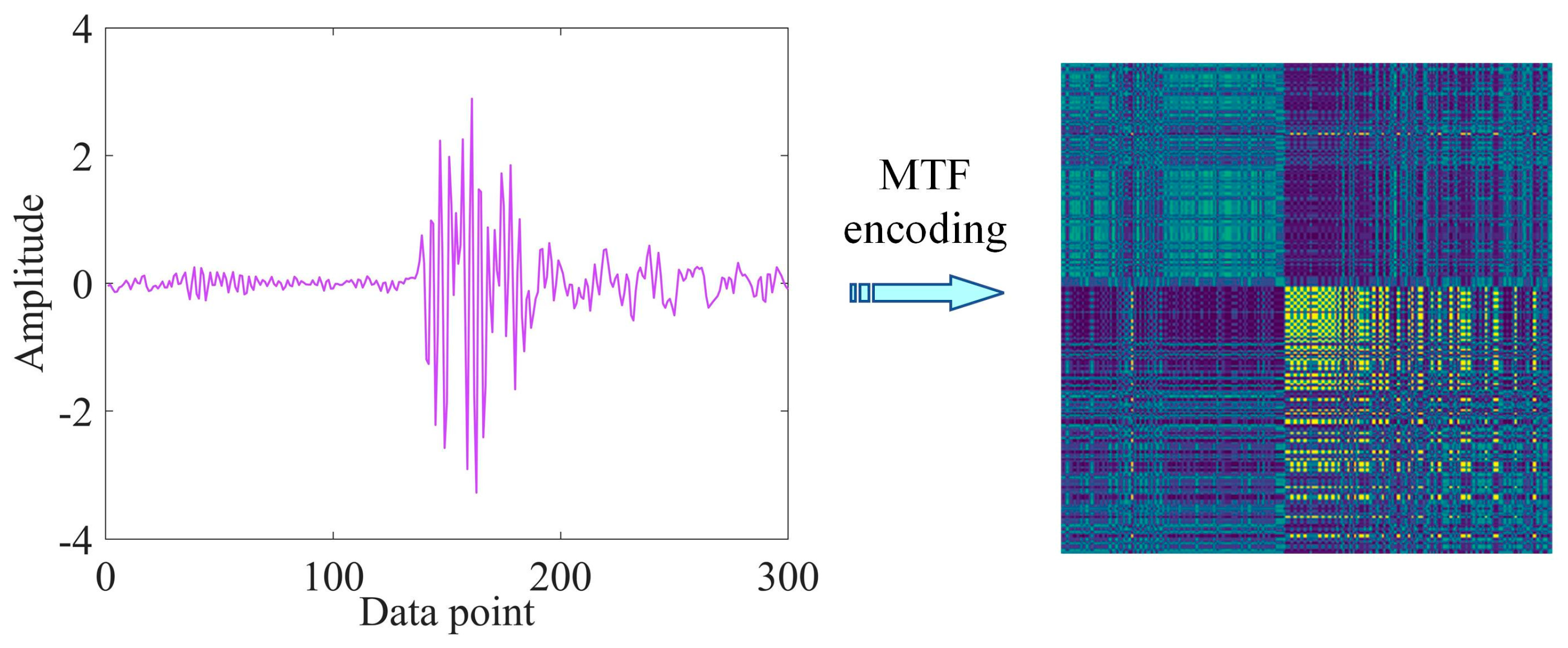
Markov Transition Field (MTF) can encode one-dimensional vibration signals into two-dimensional images [18]. It mainly uses Markov matrices to preserve time domain information and enables the encoding of dynamically transferred information. Figure 1 shows the MTF coding schematic.

Figure 1.
MTF encoding.
Given the one-dimensional time series, X = {xt, t = 1, 2, …, T}. Firstly, divide X in groups of j points; then, discretise the value domain of these points into N equal parts, where the ith part is denoted by ni (0 < i ≤ N); each point in X is mapped into a corresponding value domain ni. Finally, the transfer probability between the value domains ni of each point is calculated according to the Markov chain, and in this way, an N × N weighted neighbourhood matrix W is constructed, which can be represented as:
where the value of the element w is determined by the probability that all sequence points in the value domain nt are transferred to the value domain ni.
In order to facilitate the expression of time series features, an M × M MTF matrix is constructed according to the serial data, which can be represented as:
where the element m represents the transfer probability from the value domain nt of xi to the value domain ni of xj.
Utilising MTF as a pre-processing method can have several advantages:
- The original signal and the 2D image are coded mapping relations, avoiding the loss of information of the original signal.
- The dependency between each grouping and the time step is considered, which preserves the temporal correlation of the signal over time.
- Different colours reflect the probability of transfer between different data, and the two-dimensional space amplifies the temporal information, facilitating greater performance of the residual network.
2.2. Feature Extraction Based on Residual Network
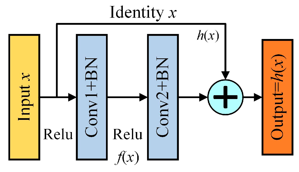
Residual networks solve the gradient vanishing and explosion problems of traditional convolutional models and are widely used as deep learning networks [19]. They have a deeper network structure for better feature extraction, and this intrinsic structure is shown in Figure 2.
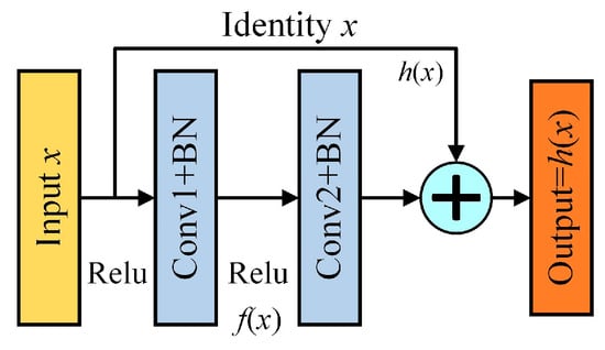
Figure 2.
Residual structure.
Where x represents the input feature matrices; f(x) represents the mapping function; Relu represents the non-linear activation function; the normalisation mode is BN; and h(x) represents the constant function, as determined by the following equation:
The feature extraction is performed by 2–3 convolutional layers on the main line of each residual structure, and the feature data on the shortcut branches can be directly added to the feature data on the main line, which can be achieved by simply assuring that input matrices x and mapping functions f(x) are of the same dimension. The cumulative stacking of residual structures increases the number of convolutional layers and improves feature extraction.
2.3. Feature Extraction Based on Attention Mechanisms
Convolutional layers of different dimensions in residual networks can be used to recognise a large amount of feature information; however, most convolutional layers process the input features in the same way, resulting in some loss. Accordingly, the model introduces two attentional mechanisms to distinguish different feature weights in terms of channel and spatial dimensions, which makes the model more enhanced for recognising the representation of the feature regions of the images [20].
2.3.1. Channel Attention-Based Feature Extraction
The channel attention mechanism identifies remote location dependencies of input data along two dimensions directions, and the channel attention structure for MARN is shown in Figure 3. The input matrices data are average pooled horizontally and vertically to compress the channel dimensions, followed by a two-layer 1 × 1 convolutional dimensionality reduction with simultaneous nonlinear activation; then, splitting along the spatial dimension is performed to obtain the direction-aware feature matrix and the location-sensitive feature matrix. Finally, the two matrices are weighted to obtain the channel attention feature matrix. This process can be represented as:
where M represents the input matrix; represents activation function; represents convolution algorithm with 1 convolutional kernel; S represents the split operation; and Avgpool represents average pooling.
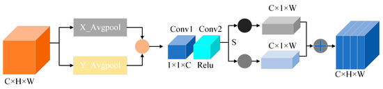
Figure 3.
Channel attention mechanism for MARN (CA, compressing and splitting the feature matrices to obtain the channel attention matrixes).
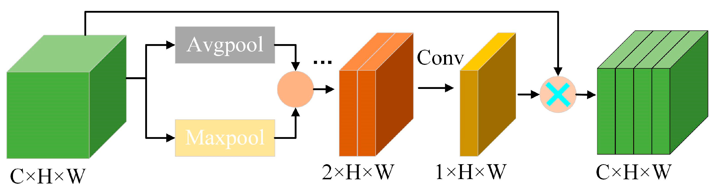
2.3.2. Spatial Attention-Based Feature Extraction
The spatial attention mechanism takes into account the different levels of importance of spatial dimensional information and ultimately results in a spatial attention feature matrix with different weights. The structure of spatial attention used for MARN is shown in Figure 4. Firstly, average and maximum pooling are used on the input data in both directions simultaneously, and subsequently, the results are spliced to generate a transition matrix, which is then downscaled using a 7 × 7 convolutional layer, and finally weighted to obtain the spatial feature matrices of the different positional information to determine the positions that need to be attended to. The specific process can be expressed as follows:
where represents the convolution algorithm with seven convolutional kernels.
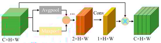
Figure 4.
Spatial attention mechanism for MARN (SA, pooling operation followed by dimensionality reduction to get the spatial feature matrixes).
3. Model Structure and Fault Diagnosis Process
This section details the MARN structure for bearing fault diagnosis and sets up the appropriate diagnostic process.
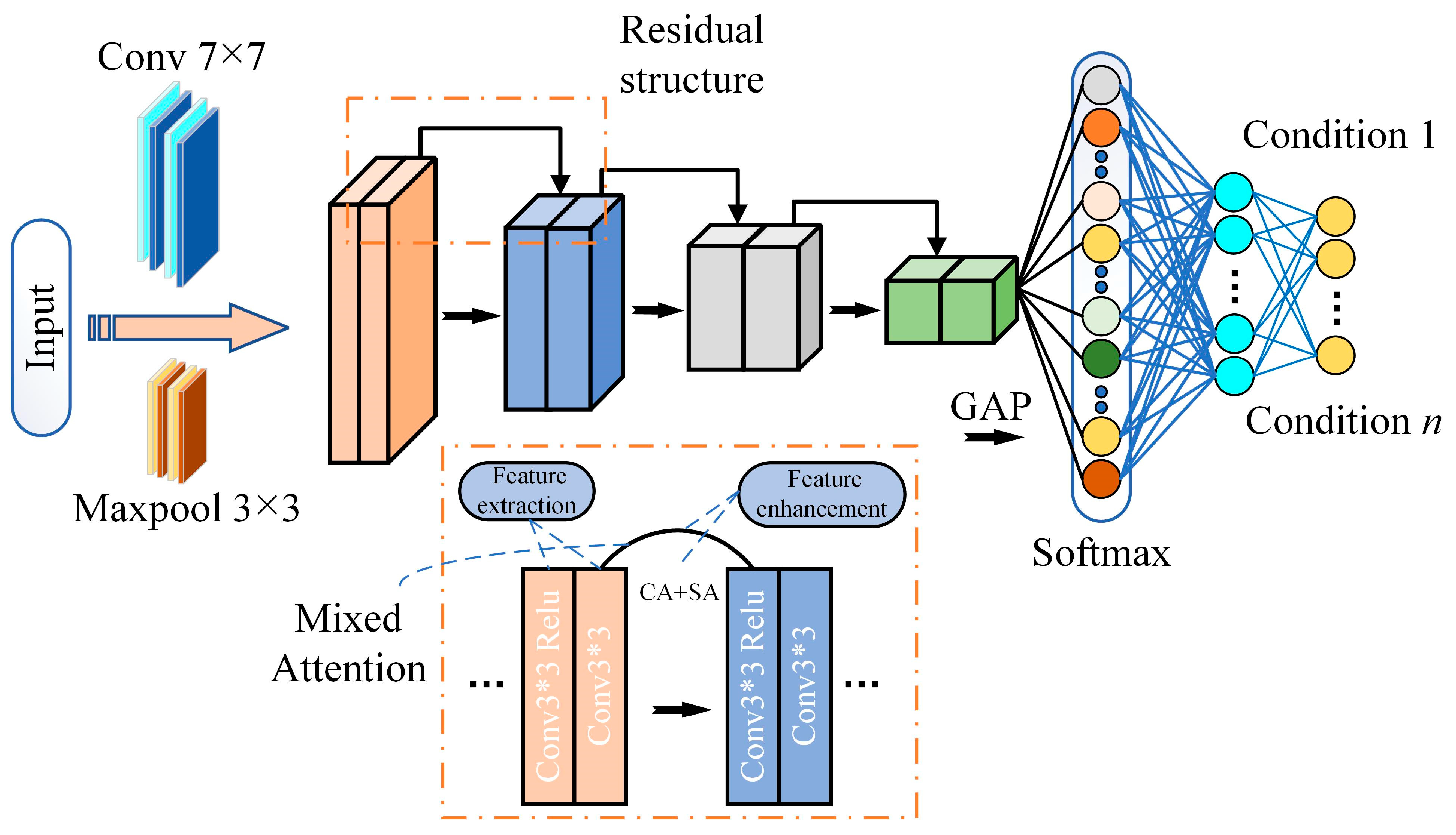
3.1. MARN Model Structure
The MARN model is shown in Figure 5, which in general consists of the residual feature extraction layers, the mixed attention feature enhancement layers and the Softmax classification layers.

Figure 5.
MARN model structure (residual structure and mixed attention mechanisms composed with fault classification by Softmax).
In order to learn as many features as possible from the input images, the feature extraction layer uses 16 groups of residual structures (each containing two 3 × 3 convolutional layers) for feature extraction; all the features extracted by the feature extraction module are subsequently passed through the feature enhancement layer to augment the representation of the features. In residual networks, a portion of the input feature matrices are passed directly from the bottom layer to the top layer, so further channel compression and refinement are required; and the top layer information obtained through mainline convolution lacks location and detail information, although it contains more global abstract information. Therefore, channel and spatial mixed attention mechanism is introduced to utilise high- and low-level information fusion enhancements to make the information more complete.
After feature enhancement, the global average pooling (GAP) is used to match each feature matrix assigned with different intrinsic meanings to the fault categories, which better integrates global spatial information and reduces the network parameters. Finally, the Softmax classifier is used to classify the faults.
3.2. Fault Diagnosis Process
The fault diagnosis process is shown in Figure 6, which can be split into the following steps:
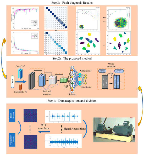
Figure 6.
Fault diagnosis process (Steps 1–3 are data preprocessing, model training, and deriving diagnostic results, respectively).
Step 1: Data acquisition and preprocessing. The vibration signals collected from the CWRU bearing data were first converted into 2D MTF-encoded images and divided into corresponding datasets (balanced and unbalanced data).
Step 2: Build and train the network. The network is built, specific parameters are set, and the dataset divided in the previous step is input into MARN for training.
Step 3: Use MARN to validate the comparison of other 1D to 2D coding methods under the same data, and verify the performance of the mixed attention mechanism.
Step 4: Compare popular fault diagnosis models on divided balanced and unbalanced datasets to validate the superiority of the proposed method.
4. Experimental Analysis
This section evaluates the effectiveness of the MTF-MARN using CWRU bearing data. All network models are trained using Python 3.7 programming with Pytorch framework, Intel Core i7-7300 CPU@3.2 GHz, GTX1050(4G) under Windows 10.
4.1. Acquisition and Division of Datasets
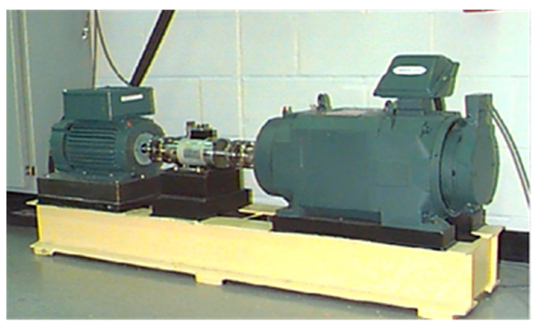
The experimental data were acquired from the CWRU bearing experimental platform (Figure 7). Taking the fan-end bearing SKF-6203 as an example, motor speed is 1772 r/min, set up single-point damage with different failure diameters for the inner ring, rolling body and outer ring (@3, @6, @12) of the bearings, respectively; and placed the sensor (sampling frequency is 48 khz) on the fan-end bearing housings for the collection of vibration signals. Three different damage diameters of the outer ring, rolling element (@6) and inner ring are selected as fault samples, and a normal sample is also included, a total of ten categories to produce the corresponding dataset. The different failure types are labelled as “IR”, “RF”, “OR”, and “NOR”.
Most equipment tend to be healthy in practice and it is difficult to obtain a large amount of labelled fault data [21]; therefore, the proposed method in this paper is trained on both balanced and unbalanced data. DatasetA (DA) can be seen as an idealised balanced dataset, while DB/DC/DD divides the different fault samples into different proportions to simulate the missing data. It is worth noting that DA takes the first 400 samples of each faulty signal segment, while DB/DC/DD are randomly selected data from DA divided into unbalanced datasets, respectively. To avoid chance occurrence, each dataset is randomly divided into training and validation sets according to 9:1, and the division strategy is shown in Table 1.

Table 1.
Four forms of division of datasets with different data distributions.

Figure 7.
CWRU bearing experiment platform [22].
Figure 7.
CWRU bearing experiment platform [22].
4.2. Data Generation Method and Training Parameter Settings
4.2.1. Data Enhancement
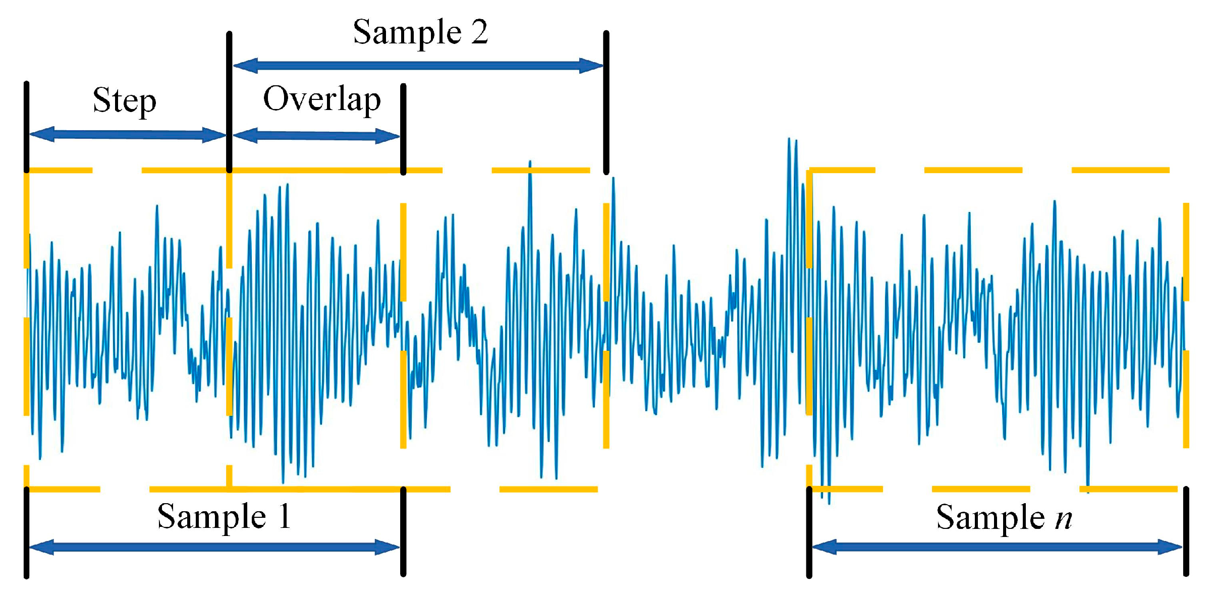
In most neural networks for fault diagnosis, data enhancement is an effective means to achieve more desirable classification accuracy and to prevent the occurrence of data overfitting. In this paper, overlapping sampling of vibration signals using sliding windows is used as a data enhancement method. The advantage of this enhancement method is that two neighbouring coded images will contain overlapping timing information, which allows the MTF to fully exploit the intrinsic temporal correlation between the overlapping signals and the two neighbouring segments before and after. The data enhancement is shown in Figure 8.
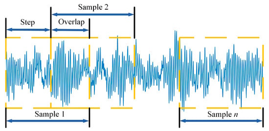
Figure 8.
Data enhancement.
Each slide of the sliding window generates an MTF image under the corresponding data to assure that each MTF coded image contains signal points for one revolution of the bearing, as determined by the following equation:
where n represents the number of points sampled per revolution of the failed bearing; R represents rotational speed, which is 1772 r/min; and Fq represents the sampling frequency of the sensor.
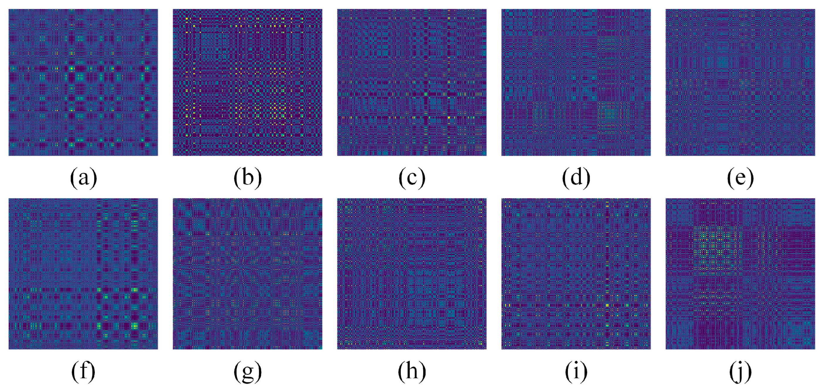
The sliding window size is calculated to be 1024 and the sliding step size is taken as 512. Considering the fact that images that are too small have compressed characteristics and images that are too large are affected by hardware devices, a 300 × 300 MTF image was generated for each sliding. Different types of fault images are shown in Figure 9.
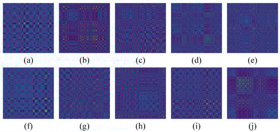
Figure 9.
MTF coded images. (a) NOR-L0; (b) IR-L1; (c) IR-L2; (d) IR-L3; (e) RF-L4; (f) RF-L5; (g) RF-L6; (h) OR-L7; (i) OR-L8; (j) OR-L9.
4.2.2. Training Parameter Settings
The training set can be image cropped and flipped during training to increase the generalisation of the model. The optimiser can guide the gradient of the loss function (LF) in the back propagation process of the model to approach the convergence continuously; in this paper, the use of the Adam optimiser can reduce the memory requirement and reduce the load of the hardware device. To avoid the model converging too slowly, the learning rate (LR) is taken as 0.001; the specific training parameters are shown in Table 2.
Table 2.
Method of setting training parameters.
4.3. Experimental Analyses
4.3.1. Comparison of Different 2D Transformation Methods
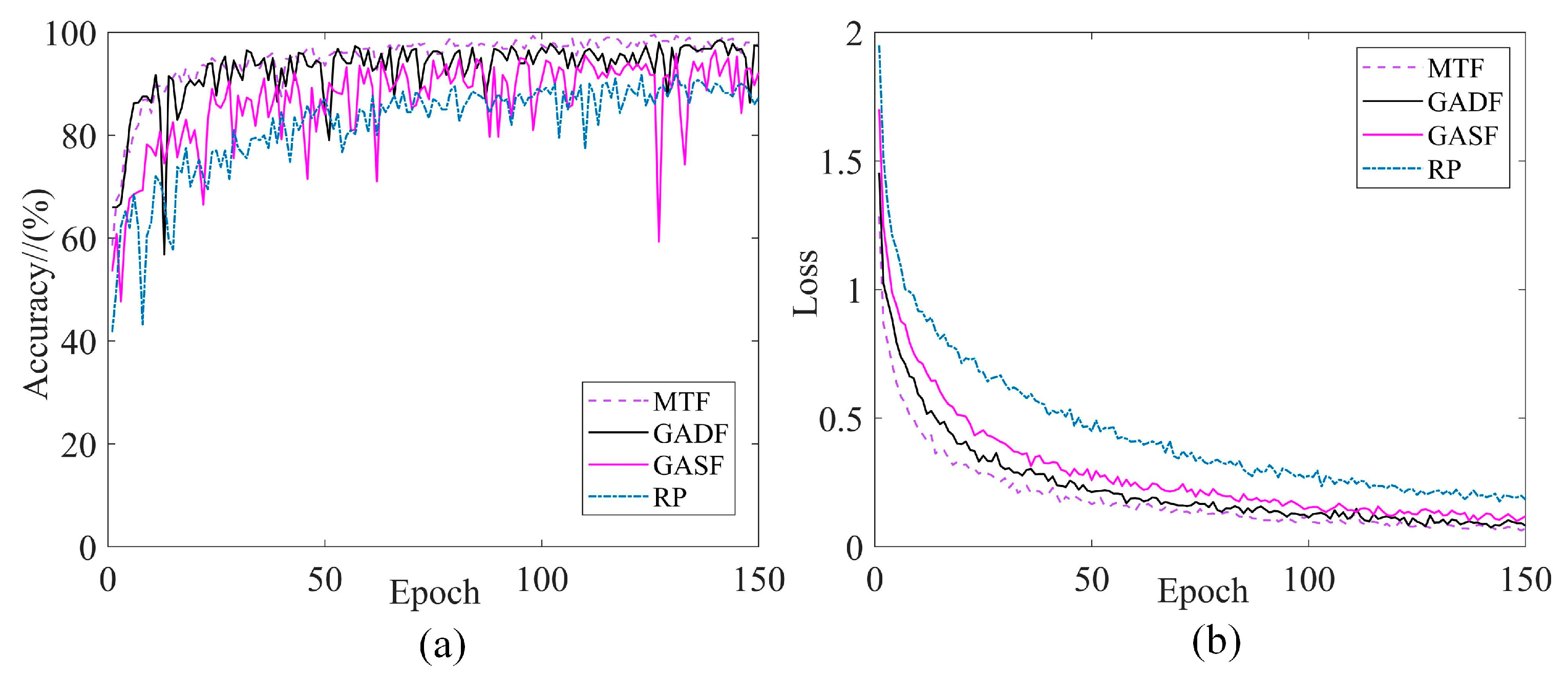
To verify the superiority of MTF as a preprocessing method, this section compares other commonly used 2D image transformation methods. Under the same original vibration signals, the corresponding datasets were generated using Gramian Angle Field (GADF/GASF) and recurrence plot (RP), respectively, and compared with the MTF method. They were inputted into the MARN model for training, respectively. Taking the balanced dataset DA as an example, 150 rounds of model iterations were performed for each set of models in order to ensure sufficient model convergence.
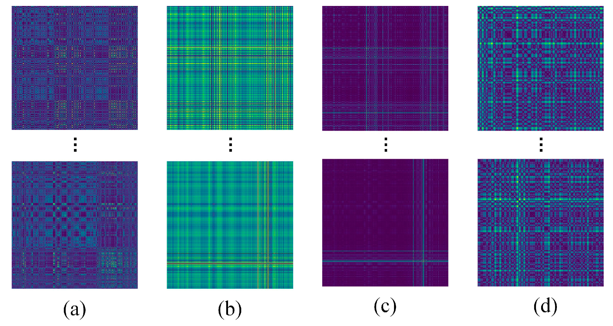
Figure 10 shows example images of several transformation methods, and Figure 11 shows the training curve of the model. As can be seen in Figure 11, using MTF as the preprocessing method has the highest validation accuracy after the same model training. Additionally, it is clear that the model is the most stable and has the lowest training loss during training using MTF as the data input, so it can be shown that several other methods are not as good as MTF in terms of characterisation.

Figure 10.
Example images of different 2D transformation methods: (a) MTF; (b) GADF; (c) GASF; (d) RP.
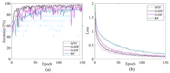
Figure 11.
Training curves for different transformation methods: (a) Validation accuracy; (b) Training loss.
To further explore the advantages of MTF as a data preprocessing method, the time used to generate each coded image and the image size were also included. Table 3 shows the comparative indicators of the different transformation methods, it can be seen that each GASF image has the smallest size and the shortest network training time, but MTF has the minimum transformation time and highest validation accuracy.
Table 3.
Comparison of indicators for different transformation methods (Bold are optimal data).
4.3.2. Comparison of Different Attention Mechanisms
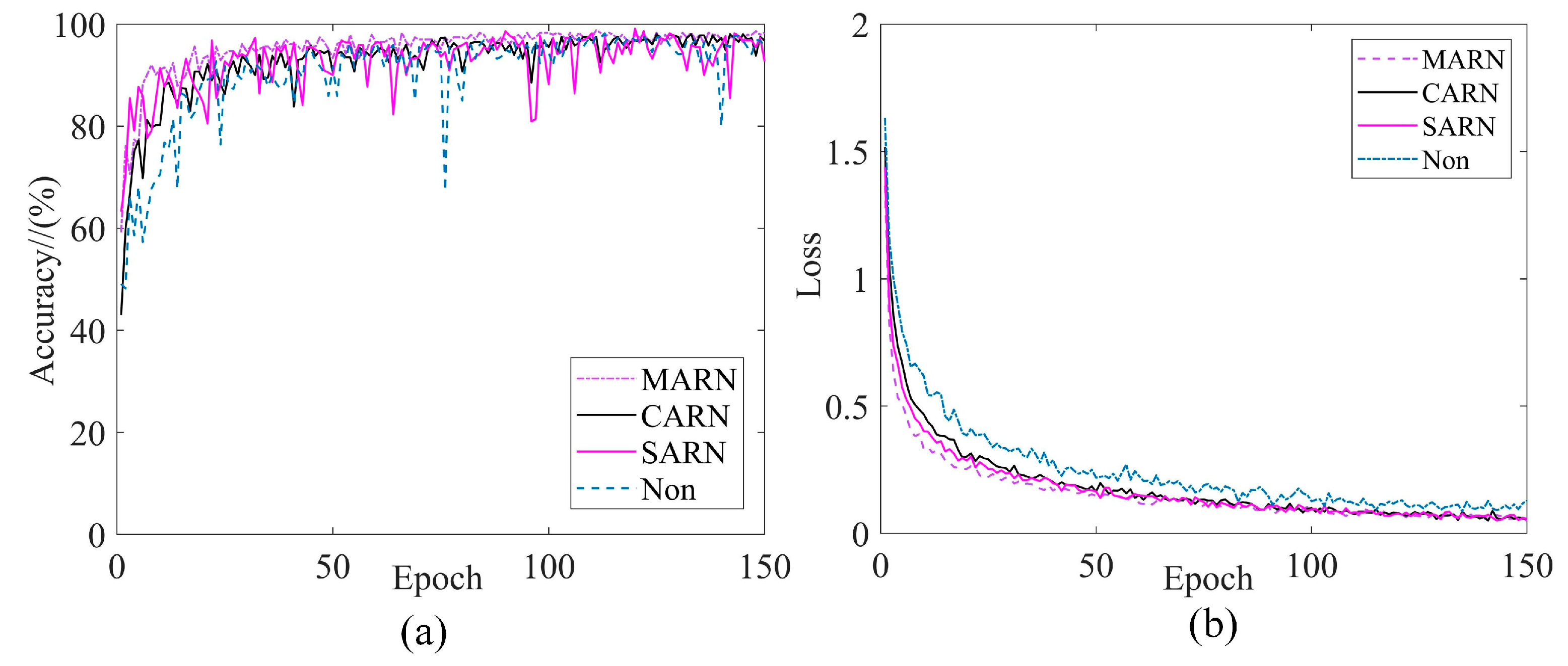
To verify the advantages of the mixed attention mechanism, residual networks built in this paper are used to embed different attention mechanisms separately for comparison. The CA and SA modules are embedded in the residual network separately, and an additional residual network without the introduction of the attention mechanism is included as a comparison model (where CA and SA are both methods proposed in the paper). Several models are iterated for 150 rounds under each of the four datasets to validate the feature recognition capability of the mixed attention mechanism.
Taking the unbalanced data DB as an example, Figure 12 shows the training performance curves of different attention mechanisms. From Figure 12, it can be seen that the mixed attention mechanism fluctuates gently and is more stable during training. In contrast, the single attention mechanism and the model without the introduction of the attention mechanism may have occasional sharp jumps during training, and the accuracy is not as good as the proposed model. Table 4 shows the maximum validation accuracies of several methods on the four datasets. It can be seen that the mixed attention mechanism achieves an optimal classification accuracy no matter under which data distribution. Therefore, it can be demonstrated that the mixed attention mechanism is capable of more stable feature recognition.
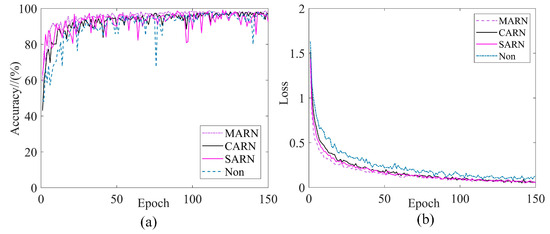
Figure 12.
Training curves for different attention mechanisms: (a) Validation accuracy; (b) training loss.
Table 4.
Maximum validation accuracy of different attention mechanisms under four datasets (Bold are optimal data).
4.3.3. Visualisation Analysis
Figure 13 shows the classification confusion matrices of MARN under the four datasets. The horizontal and vertical coordinates of the confusion matrix represent the true and predicted labels, respectively, and diagonal numbers represent the prediction accuracies of two labels. Taking the randomly divided validation set as example, it can be seen that label2 has the lowest accuracy in DA and DC, label4 has the lowest accuracy in DB and DD, and the other labels are able to achieve full classification. The reason for the individual misclassification of labels is that some sample images are more similar to other categories, but overall MARN has excellent fault classification capabilities.
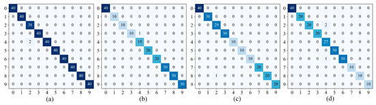
Figure 13.
Confusion matrices: (a) DA; (b) DB; (c) DC; (d) DD.
The method of t-SNE dimensionality reduction (Figure 14) can be used to visualise the classification effect of the MARN.
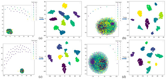
Figure 14.
t-SNE dimensionality reduction: (a) DA; (b) DB; (c) DC; (d) DD.
In the left half of each subgraph is the original feature distribution of each dataset (training set), and the right half is the feature classification result of the fully connected layer after training by the MARN (different colours represent different fault categories). From the figure, it can be seen that the dataset is haphazardly distributed in the feature space before training, and after training, the fault features of each category become uniformly clustered. There is no significant overlap between different categories, so the MARN has a good classification effect on balanced/unbalanced fault data.
4.3.4. Comparison with Existing Popular Models
In this section, to validate the superiority of MARN, several relevant models using 2D images as input data are compared. Yan et al. and He et al. used an algorithm combining MTF with residual network [23,24]; Wang et al. used a new MTF-CNN method for fault diagnosis in complex working conditions [25]; Gu et al. proposed an improved model MTF-SE-ResNet for the diagnosis of bearings under compound faults [26]; Wei et al. proposed a GADF with an improved channel attention model (FcaNet) [17]; Gu et al. proposed a RP and MobileNet-v3 for fault diagnosis of variable speed bearings [27].
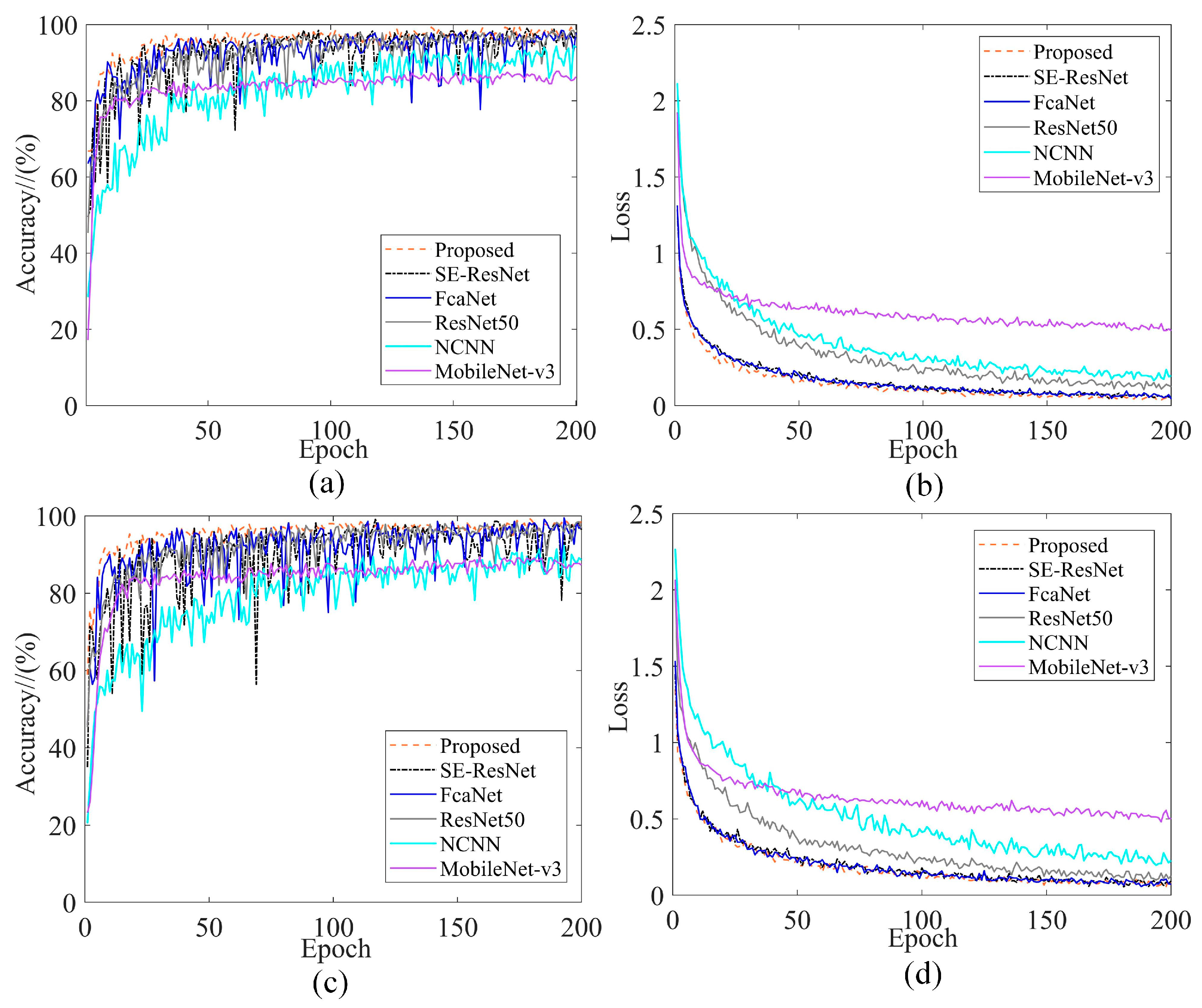
To ensure fairness in model training, the same dataset is used as input for the different networks, with the same training settings for each model. To ensure that the models converged sufficiently, 200 rounds of iterations of each model are performed. The balanced dataset DA and unbalanced dataset DB are taken as examples, respectively, and the corresponding training performance curves are shown in Figure 15. Table 5 shows the maximum validation accuracy of different methods on the four datasets.
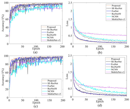
Figure 15.
Training performance curves comparing different models: (a) DA validation accuracy; (b) DA training loss; (c) DB validation accuracy; (d) DB training loss.
Table 5.
Highest validation accuracy of different methods on four datasets (Bold are optimal data).
As can be seen in Figure 15, all models have higher loss and training fluctuations on the unbalanced dataset than on the balanced dataset, which is due to the fact that a smaller amount of data has an indispensable effect on the models in terms of deep learning. Although the lightweight model MobileNet-v3 converged the fastest, the highest validation accuracy is only about 89% and has the highest training loss; this is due to the intrinsic structure of the model resulting in inadequate feature extraction. The shallow model NCNN tends to converge steadily during training, but converges too slowly, requires more iterations, and has higher training losses. Although the training loss of SE-ResNet and FcaNet is close to the proposed method, the training is not stable enough, with occasional sharp fluctuations during the training process. ResNet50 uses a deeper structure for feature extraction, and the loss is instead higher, thus illustrating that increasing the depth of the model does not necessarily result in effective feature extraction. Therefore, the proposed method can keep the loss low and the fluctuation stable regardless of the dataset.
From Table 5, it can be seen that the highest validation accuracy of FcaNet on unbalanced datasets DB and DD is the same as the proposed method; and the other methods are not as good as the present model on different datasets. Therefore, the proposed method can extract more features.
In the field of DL, evaluation metrics are the criteria for determining the performance of a model, so it is important to compare the classification metrics of different models. Accuracy Ac, precision Pr, recall Re, and F1 score are all criteria for determining the performance of the model, determined by Equations (7)–(10).
where TP and TN are the number of correct predictions in 10 categories; FP and FN are the numbers of incorrect predictions in 10 categories.
To study the advantages and disadvantages of each model more intuitively, Table 6, Table 7, Table 8 and Table 9 show the training performance metrics of the different models under the four datasets. For a more comprehensive analysis, the training time of the different models is also introduced.
Table 6.
Training metrics for different models on the DA (Bold are optimal data).
Table 7.
Training metrics for different models on the DB (Bold are optimal data).
Table 8.
Training metrics for different models on the DC (Bold are optimal data).
Table 9.
Training metrics for different models on the DD (Bold are optimal data).
As can be seen from Table 6, Table 7, Table 8 and Table 9; Pr on DB; and DD, F1 on DB, the proposed model is not as good as FcaNet, and the other metrics are better than the other models. It is also easy to see that the training time of the proposed method is longer and much higher than the shallow model, but this phenomenon will be improved with the updating of hardware equipment. Overall, the MARN is applicable to the field of fault diagnosis.
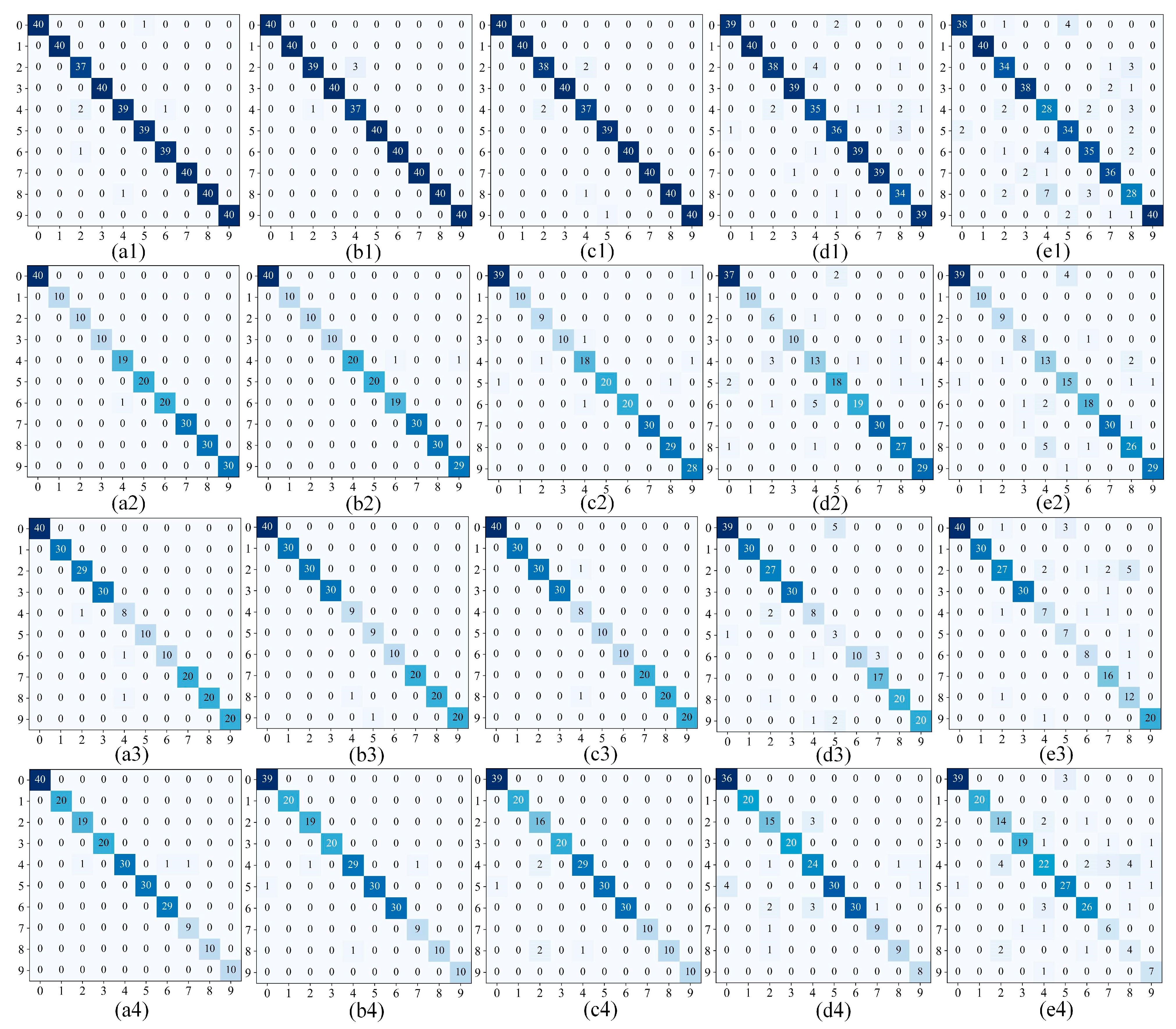
To further explore the classification effects inherent in each model, Figure 16 and Figure 17 show the confusion matrices and t-SNE dimensionality reduction in the fully connected layers for the different methods. From Figure 16(a4), it can be seen that although FcaNet achieves the same accuracy as the proposed method on DD, FcaNet misclassifies two labels, and the proposed method misclassifies only one label; the other models have large-scale misclassification on most of the labels.
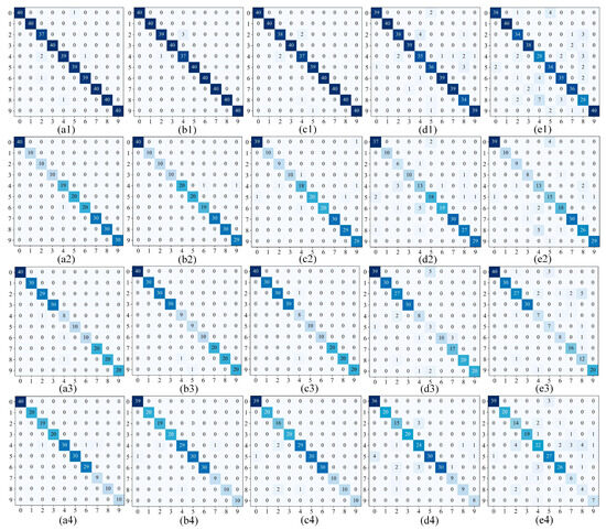
Figure 16.
Confusion matrices comparing different methods. (From (a–e) for FcaNet/SE-ResNet/ResNet50/NCNN/MobileNet-v3, and from (1–4) for DA–DD, respectively).
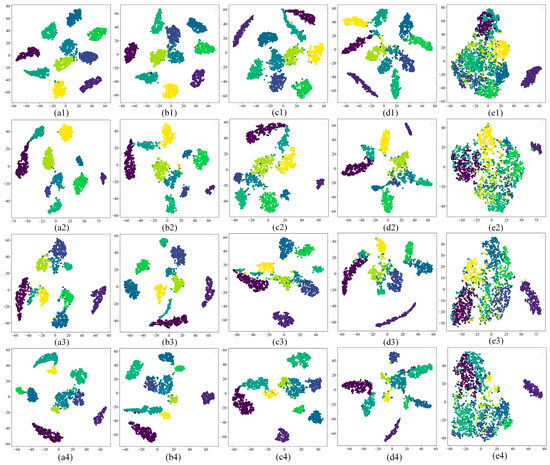
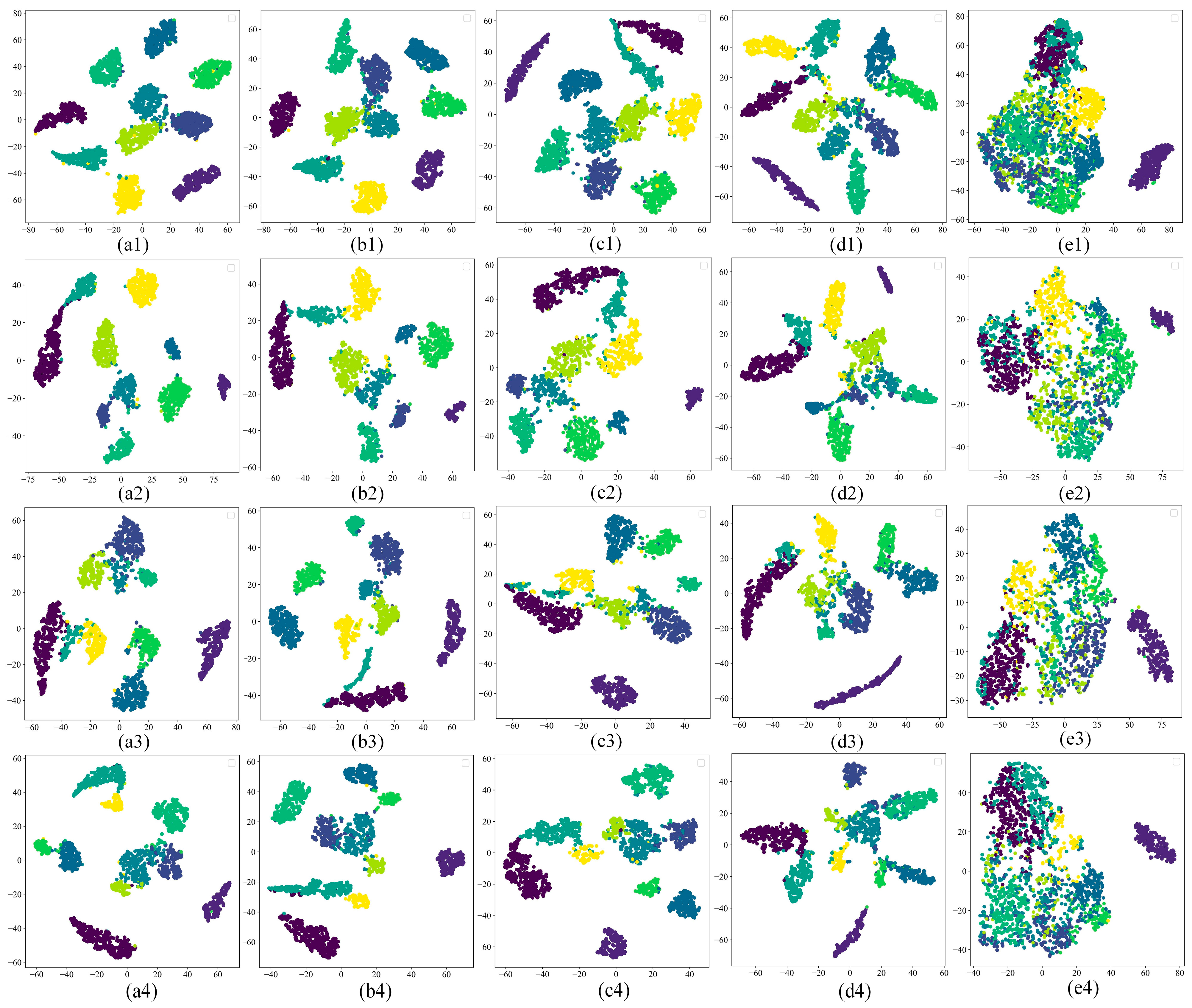
Figure 17.
Comparison of different methods for t-SNE (from (a–e) for FcaNet/SE-ResNet/ResNet50/NCNN/MobileNet-v3, and from (1–4) for DA–DD, respectively).
As can be seen from Figure 17(e1–e4), MobileNet-v3 performs very poorly in the all-connected layer clustering visualisation, with large-scale fault features undergoing confounding. While other models can achieve clustering of different classes of fault features, there is still a small amount of conflation between individual labels. Compared with the proposed method clustering, it still needs further improvement. Therefore, MARN has clear advantages in the field of fault diagnosis.
5. Conclusions
To solve most of the methods that are difficult to effectively extract fault features and unstable model training under unbalanced data, this paper proposes a new rolling bearings fault diagnosis method based on MTF and MARN, draws the following conclusions:
- The vibration signals are converted into two-dimensional images using MTF to avoid the loss of original signal information, while retaining the temporal correlation.
- Using the residual structure as the body of the network avoids the degradation problem of the model; meanwhile, the introduction of the mixed attention mechanism can enhance the feature extraction ability.
- The superiority of MTF as a data preprocessing method was confirmed on the CWRU bearing dataset, which further confirmed that the mixed attention mechanism can extract more features.
- The model performs stably on the unbalanced dataset, obtaining average recognition accuracies of 99.5% and 99.2% on the divided balanced and unbalanced data, respectively.
Although the proposed method has been improved at both the data level and the model level, diagnostic unbalanced data also have excellent fault diagnosis results; the MARN is trained from the beginning and needs a longer training period. In further research, the use of transfer learning methods can be considered to decrease training time. Moreover, the MTF-MARN method should also be used for datasets with complex operating conditions, such as strong noise and variable operating fault datasets.
Author Contributions
Conceptualization, L.X. and A.T.; methodology, A.T. and J.Z.; software, A.T.; validation, A.T., D.W. and L.X.; resources, D.W.; writing—original draft preparation, A.T.; writing—review and editing, A.T., J.Z. and D.W.; visualization, A.T.; supervision, L.X. and J.Z. All authors have read and agreed to the published version of the manuscript.
Funding
This work was supported by the National Science and Technology Major Project of China (J2019-IV-0002-0069).
Institutional Review Board Statement
Not applicable.
Informed Consent Statement
Not applicable.
Data Availability Statement
Case Western Reserve University Bearing Data. https://engineering.case.edu/bearingdatacenter (accessed on 25 December 2023).
Conflicts of Interest
The authors declare no conflicts of interest.
References
- Talhaoui, H.; Ameid, T.; Aissa, O.; Kessal, A. Wavelet packet and fuzzy logic theory for automatic fault detection in induction motor. Soft Comput. 2022, 26, 11935–11949. [Google Scholar] [CrossRef] [PubMed]
- Zhang, J.; Wu, J.; Hu, B. Intelligent fault diagnosis of rolling bearings using variational mode decomposition and self-organizing feature map. J. Vib. Control 2020, 26, 1886–1897. [Google Scholar] [CrossRef]
- Khan, S.; Yairi, T. A review on the application of deep learning in system health management. Mech. Syst. Signal Process. 2018, 107, 241–265. [Google Scholar] [CrossRef]
- Hu, Y.; Li, J.; Li, J.; Zhao, X.; Ma, B.; Dong, M. Fault diagnosis of rolling bearing based on SEMD and ISSA-KELMC. Meas. Sci. Technol. 2024, 35, 056127. [Google Scholar] [CrossRef]
- Shen, Z.; Kong, X.; Cheng, L.; Wang, R.; Zhu, Y. Fault Diagnosis of the Rolling Bearing by a Multi-Task Deep Learning Method Based on a Classifier Generative Adversarial Network. Sensors 2024, 24, 1290. [Google Scholar] [CrossRef] [PubMed]
- Imane, M.; Rahmoune, C.; Benazzouz, D. Rolling bearing fault feature selection based on standard deviation and random forest classifier using vibration signals. Adv. Mech. Eng. 2023, 15, 1–11. [Google Scholar] [CrossRef]
- Prosvirin, A.E.; Ahmad, Z.; Kim, J.M. Global and local feature extraction using a convolutional autoencoder and neural networks for diagnosing centrifugal pump mechanical faults. IEEE Access 2021, 9, 65838–65854. [Google Scholar] [CrossRef]
- Sun, H.; Fan, Y. Fault diagnosis of rolling bearings based on CNN and LSTM networks under mixed load and noise. Multimed. Tools Appl. 2023, 28, 43543. [Google Scholar] [CrossRef]
- Wang, B.; Qiu, W.; Hu, X.; Wang, W. A rolling bearing fault diagnosis technique based on recurrence quantification analysis and Bayesian optimization SVM. Appl. Soft Comput. 2024, 156, 111506. [Google Scholar] [CrossRef]
- Zhao, K.; Wu, S. An improved rolling bearing fault diagnosis method using DenseNet-BLSTM. SIViP, 2024; early access. [Google Scholar] [CrossRef]
- Zhang, T.; Chen, J.; Li, F. Intelligent fault diagnosis of machines with small & imbalanced data: A state-of-the-art review and possible extensions. ISA Trans. 2022, 119, 152–171. [Google Scholar] [CrossRef]
- Gong, X.; Feng, K.; Du, W.; Li, B.; Fei, H. An imbalance multi-faults data transfer learning diagnosis method based on finite element simulation optimization model of rolling bearing. Proc. Inst. Mech. Eng. Part C J. Mech. Eng. Sc, 2024; early access. [Google Scholar] [CrossRef]
- Zhang, W.; Li, X.; Jia, X. Machinery fault diagnosis with imbalanced data using deep generative adversarial networks. Measurement 2020, 152, 107377. [Google Scholar] [CrossRef]
- Luo, J.; Huang, J.; Li, H. A case study of conditional deep convolutional generative adversarial networks in machine fault diagnosis. J. Intell. Manuf. 2021, 32, 407–425. [Google Scholar] [CrossRef]
- Lu, J.; Wu, W.; Huang, X.; Yin, Q.; Yang, K.; Li, S. A modified active learning intelligent fault diagnosis method for rolling bearings with unbalanced samples. Adv. Eng. Inform. 2024, 60, 102397. [Google Scholar] [CrossRef]
- Qin, Z.; Huang, F.; Pan, J.; Niu, J.; Qin, H. Improved Generative Adversarial Network for Bearing Fault Diagnosis with a Small Number of Data and Unbalanced Data. Symmetry 2024, 16, 358. [Google Scholar] [CrossRef]
- Wei, L.; Peng, X.; Cao, Y. Rolling bearing fault diagnosis based on Gramian angular difference field and improved channel attention model. PeerJ Comput. Sci. 2024, 10, 1807. [Google Scholar] [CrossRef]
- Lei, C.; Miao, C.; Wan, H.; Zhou, J.; Hao, D.; Feng, R. Rolling bearing fault diagnosis method based on MTF-MFACNN. Meas. Sci. Technol. 2024, 35, 035007. [Google Scholar] [CrossRef]
- Tong, A.; Zhang, J.; Xie, L. Intelligent Fault Diagnosis of Rolling Bearing Based on Gramian Angular Difference Field and Improved Dual Attention Residual Network. Sensors 2024, 24, 2156. [Google Scholar] [CrossRef]
- Li, B.; Ren, H.; Jiang, X.; Miao, F.; Feng, F. SCEP—A new image dimensional emotion recognition model based on spatial and channel-wise attention mechanisms. IEEE Access 2021, 9, 25278–25290. [Google Scholar] [CrossRef]
- Zhao, K.; Jia, F.; Shao, H. Unbalanced fault diagnosis of rolling bearings using transfer adaptive boosting with squeeze-and-excitation attention convolutional neural network. Meas. Sci. Technol. 2023, 34, 044006. [Google Scholar] [CrossRef]
- Case Western Reserve University Bearing Data Center [EB/OL]. 2018. Available online: https://engineering.case.edu/bearingdatacenter/apparatus-and-procedures (accessed on 25 December 2023).
- Yan, J.; Kan, J.; Luo, H. Rolling Bearing Fault Diagnosis Based on Markov Transition Field and Residual Network. Sensors 2022, 22, 3936. [Google Scholar] [CrossRef]
- He, K.; Xu, Y.; Wang, Y.; Wang, J.; Xie, T. Intelligent Diagnosis of Rolling Bearings Fault Based on Multisignal Fusion and MTF-ResNet. Sensors 2023, 23, 6281. [Google Scholar] [CrossRef] [PubMed]
- Wang, M.; Wang, W.; Zhang, X.; Iu, H.H.-C. A New Fault Diagnosis of Rolling Bearing Based on Markov Transition Field and CNN. Entropy 2022, 24, 751. [Google Scholar] [CrossRef] [PubMed]
- Gu, X.; Tian, Y.; Li, C.; Wei, Y.; Li, D. Improved SE-ResNet Acoustic–Vibration Fusion for Rolling Bearing Composite Fault Diagnosis. Appl. Sci. 2024, 14, 2182. [Google Scholar] [CrossRef]
- Gu, Y.; Chen, R.; Wu, K.; Huang, P.; Qiu, G. A variable-speed-condition bearing fault diagnosis methodology with recurrence plot coding and MobileNet-v3 model. Rev. Sci. Instrum. 2023, 94, 034710. [Google Scholar] [CrossRef] [PubMed]


Disclaimer/Publisher’s Note: The statements, opinions and data contained in all publications are solely those of the individual author(s) and contributor(s) and not of MDPI and/or the editor(s). MDPI and/or the editor(s) disclaim responsibility for any injury to people or property resulting from any ideas, methods, instructions or products referred to in the content. |
© 2024 by the authors. Licensee MDPI, Basel, Switzerland. This article is an open access article distributed under the terms and conditions of the Creative Commons Attribution (CC BY) license (https://creativecommons.org/licenses/by/4.0/).